HAL Id: hal-02368304
https://hal.archives-ouvertes.fr/hal-02368304
Submitted on 18 Nov 2019HAL is a multi-disciplinary open access archive for the deposit and dissemination of sci-entific research documents, whether they are pub-lished or not. The documents may come from teaching and research institutions in France or abroad, or from public or private research centers.
L’archive ouverte pluridisciplinaire HAL, est destinée au dépôt et à la diffusion de documents scientifiques de niveau recherche, publiés ou non, émanant des établissements d’enseignement et de recherche français ou étrangers, des laboratoires publics ou privés.
Correlations between plant climate optima across
different spatial scales
C. Johan Dahlberg, Johan Ehrlén, Ditte Marie Christiansen, Eric Meineri,
Kristoffer Hylander
To cite this version:
C. Johan Dahlberg, Johan Ehrlén, Ditte Marie Christiansen, Eric Meineri, Kristoffer Hylander. Corre-lations between plant climate optima across different spatial scales. Environmental and Experimental Botany, Elsevier, 2020, pp.103899. �10.1016/j.envexpbot.2019.103899�. �hal-02368304�
1 1
Correlations between plant climate optima across different
2
spatial scales
3
4 5
C. Johan Dahlberg1,2, Johan Ehrlén1,3, Ditte Marie Christiansen1,3, Eric Meineri4, Kristoffer 6
Hylander1,3,* 7
8
1
Department of Ecology, Environment and Plant Sciences, Stockholm University, 9
SE-106 91 Stockholm, Sweden 10
2
present address: the County Administrative Board of Västra Götaland, SE-403 40 11
Gothenburg, Sweden 12
3
Bolin Centre for Climate Research, Stockholm University, SE-106 91 Stockholm, Sweden 13
4
Aix Marseille Univ, Avignon Université, CNRS, IRD, IMBE, Marseille, France 14
* Corresponding author: Department of Ecology, Environment and Plant Sciences, Stockholm 15
University, SE-106 91 Stockholm, Sweden 16
Esitémail: [email protected] 17
18
Short running heading: Correlations between climatic optima across scales 19
20 21 22 23
2
Abstract
24
Identifying the factors determining the abundance and distribution of species is a fundamental 25
question in ecology. One key issue is how similar the factors determining species’ 26
distributions across spatial scales are (here we focus especially on spatial extents). If the 27
factors are similar across extents, then the large scale distribution pattern of a species may 28
provide information about its local habitat requirements, and vice versa. We assessed the 29
relationships between landscape and national optima as well as landscape and continental 30
optima for growing degree days, maximum temperature and minimum temperature for 96 31
bryophytes and 50 vascular plants. For this set of species, we derived landscape optima from 32
abundance weighted temperature data using species inventories in central Sweden and a fine-33
grained temperature model (50 m), national optima from niche centroid modelling based on 34
GBIF data from Sweden and the same fine-grained climate model, and continental optima 35
using the same method as for the national optima but from GBIF data from Europe and 36
Worldclim temperatures (c. 1000 m). The landscape optima of all species were positively 37
correlated with national as well as continental optima for maximum temperature (r=0.45 and 38
0.46, respectively), weakly so for growing degree days (r = 0.30 and r = 0.28), but sometimes 39
absent for minimum temperature (r=0.26 and r = 0.04). The regression slopes of national or 40
continental optima on local optima did not differ between vascular plants and bryophytes for 41
GDD and Tmax. However, the relationship between the optima of Tmin differed between 42
groups, being positive in vascular plants but absent in bryophytes. Our results suggest that 43
positive correlations between optima at different spatial scales are present for some climatic 44
variables but not for others. Moreover, our results for vascular plants and bryophytes suggest 45
that correlations might differ between organism groups and depend on the ecology of the 46
focal organisms. This implies that it is not possible to routinely up- or downscale distribution 47
3
patterns based on environmental correlations, since drivers of distribution patterns might 48
differ across spatial extents. 49
Keywords: bryophyte; climatic optima; distribution; microclimate; spatial scale; vascular
50
plant 51
4
1. Introduction
52
Identifying the factors determining the abundance and distribution of species, and and if those 53
environmental factors remain important across spatial scale (grain and extent) are key 54
objectives in global change ecology (Hurlbert et al., 2005; Hess et al., 2006; Azaele et al., 55
2015). Given that populations in different parts of the distribution range are genetically 56
similar and experience the same range of environmental conditions, we would expect that the 57
relationship between environmental factors and distributions should be similar in different 58
parts and over different spatial extents (e.g. Brown, 1984; Guisan and Zimmermann, 2000; 59
Thuiller et al. 2005; Wiens et al., 2010; Wasof et al., 2015). Yet, there are several reasons 60
why we should instead expect relationships to differ among different parts of the distribution 61
range or among different spatial extents. First, populations in different part of the distribution 62
range might be genetically differentiated and locally adapted with regard to the relationship 63
between environmental conditions (including biotic interactions) and individual performance 64
(Lavergne et al., 2010; Pellissier et al., 2013). For example, Alberto et al. (2013) found 65
genetic differentiation of many adaptive traits when comparing populations of many tree 66
species across geographically separated common gardens. Second, the frequency distribution 67
and range of environmental parameters influencing organism performance as well as the 68
correlation between parameters will often vary among different parts of the distribution range 69
and between extents of different sizes (Hylander et al. 2015). Third, distributions might not be 70
in equilibrium with current environmental conditions. For example, environmental conditions 71
might have changed but changes in distribution are time-lagged due to dispersal limitation or 72
delayed extinctions (Svenning et al. 2015) and such processes are likely to vary among spatial 73
scales. Moreover, changing the grain size of environmental predictors often results in changes 74
in which environmental variables that best predict distributions. For example, structural 75
habitat variables were more important predictors than climate variables in predicting the 76
5
distribution of an ant species at finer scales (grain), while the reversed was true at larger 77
spatial grain sizes (Menke et al. 2009). Since organisms always interacts with their local 78
environment, it is important to use fine grained data, and this is not least true for climate 79
variables (Keppel et al 2012; Lenoir et al. 2013; Lenoir et al. 2017; Hannah et al., 2014; 80
Meineri et al., 2015; Lembrechts et al 2018). However, also when we have access to such 81
fine-grained environmental data, it is not trivial to downscale organisms distributions since 82
high resolution occurrence data are still uncommon (Menke et al. 2009, Keil et al. 2013). 83
Given that the relationship between environmental factors and distributions might 84
differ over different spatial scales, a key task is to empirically assess if the factors governing 85
distributions (and optima) are similar over different spatial grains and extents, as well as how 86
such relationships differ among species and environmental variables. One important question 87
regards how the strength of the relationships between distributions and environmental factors 88
(e.g. species optima) differ among spatial grains and extents. If the relationship is strong, then 89
the large scale distribution pattern of a species may provide information about its local habitat 90
requirements, and vice versa. Another important question is if relationships, and thus the 91
predictive capacity, are stronger for some environmental variables than for others. Lastly, 92
relationships with a given environmental factor can vary between groups of species with 93
different physiology. For example, moisture conditions are probably more important for 94
bryophytes than for vascular plants, since bryophytes cannot regulate water uptake and loss 95
(cf. Woodward and Williams, 1987; Hylander, 2005; Proctor, 2011), or winter conditions 96
might be more important for trees than for herbs in areas with snow cover (Walter and 97
Breckle, 1989).
98
In this study, we investigated how strongly temperature optima of 50 vascular plant 99
species and 96 bryophyte species were correlated between spatial scales. We compared 100
optimqfrom a landscape consisting of 3000 km2 forested area in central Sweden, with the 101
6
optima calculated at the national extent using a fine-grain climate data, and with optima at a 102
continental extent including most of Europe with a more coarse-grain climate data. Three 103
temperature variables were examined: growing degree days, minimum temperature and 104
maximum temperature. We retrieved the species’ landscape optima, defined as the most 105
favorable climate in the focal landscape, by calculating abundance-weighted temperature 106
averages for georeferenced species occurrences from 49 inventoried field sites. The national 107
and continental optima were retrieved from niche centroid modelling (Blonder et al. 2017), 108
and reported occurrences in Europe of the same species’ in a database. Using these three 109
optima from different geographic extents, we examined the strength of correlations for the 110
three climate variables, for all species pooled as well as for vascular plants and bryophytes 111
separately. 112
113
2. Materials and Methods
114
2.1 Study areas 115
The study area used for the landscape scale data is located in the county of Ångermanland in 116
central Sweden (Fig. 1a; between the latitudes 62°50’ and 63°12’ N). This area ranges 73 km 117
westward from the Baltic Sea and 42 km from north to south. The area is hilly with a 118
moderate altitudinal variation (0 – 470 m). The bedrock consists mostly of gneiss covered by 119
podzolic soils of sandy loamy or silty materials. It is a mainly forested landscape situated in 120
the middle boreal subzone, and, along the coast, in the southern boreal subzone. In July, the 121
mean temperature is 15.6 °C, and the annual mean precipitation reaches 671 mm (Swedish 122
Meteorological and Hydrological Institute, 2016). The heterogeneous topography and the fact 123
that this area hosts the range margins of both southern and northern species (Mascher, 1990) 124
make this a particularly suitable landscape to study the influence of microclimate on species 125
distributions. 126
7
The whole of Sweden (450 000 km2) was used to examine the national scale. Sweden 127
is extending over a substantial latitudinal and altitudinal gradient (latitudes 55.3 - 69.1°N and 128
0-2100 m.a.s.l). The continental scale study area comprises a large part of Europe, is more 129
than 5100 km from west to east and 2800 km from south to north, and cover a land area of 130
4.40 × 10⁶ km2 (Fig. 1b, between the latitudes 27°38’ and 81°48’ N). It covers a wide range of 131
altitudes (up to 4810 m.a.s.l.) and climatic conditions from Mediterranean climate in the south 132
to cold climates with long winters in the north and at high altitudes. There is also an east-west 133
climatic gradient across the temperate zone ranging from maritime climates along the Atlantic 134
Ocean to continental climates in the eastern inlands (Peel et al., 2007; Europe, 2014). 135
136
2.2 Study design and species occurrences 137
In the focal landscape, we selected 24 south-facing and 25 north-facing forested slopes 138
distributed across the whole area. Within each slope, we randomly selected one 25 × 25m plot 139
within mature forest (at least 50 years old, estimated from aerial pictures). To reduce 140
environmental heterogeneity, selected plots were located > 25 m from open areas, > 50 m 141
from streams, > 10 m from vertical cliffs (> 5 m high), and were situated on mesic soils. Most 142
of the plots were dominated by Norway spruce (Picea abies L. Karst.), but at some sites also 143
birch (Betula pubescens Ehrh. and Betula pendula Roth), Aspen (Populus tremula L.) or 144
Scots pine (Pinus sylvestris L.) co-dominated the tree layer. The plots were oriented between 145
159° and 214° at south-facing slopes (180° = S) and between 333° and 56° at north facing 146
slopes (360°/0° = N). The slope inclination varied between 7° and 35°, and the altitude ranged 147
from 39 m to 385 m. We assessed the local area species composition within each of the 49 148
chosen 25 × 25 m plots by recording the abundance of all occurring species of bryophytes and 149
vascular plants. We estimated the abundance in three categories 1 = sporadic (few 150
occurrences covering < 5 %), 2 = common (covering 5 – 50 %), and 3 = dominant (covering ≥ 151
8
50 %). For analyses of optima, we included all bryophyte and vascular plant species occurring 152
in at least 5 of the plots (Appendix S1), resulting in 96 bryophytes and 50 vascular plant 153
species. 154
For the national scale we compiled occurrences of the study species from Swedish 155
Artportalen (www.artportalen.se) and for the continental scale also from GBIF 156
(www.gbif.org), and Norwegian Artsobservasjoner (www.artsobservasjoner.no). In GBIF, we 157
included observations, literature data and herbarium specimens. We restricted the GBIF 158
occurrence data sets to the time period 1950 to 2014. Information on the precision of 159
coordinates was lacking for large parts of the GBIF data sets and to include as many 160
observations as possible, we did not apply any restrictions on precision. In the continental 161
scale data we included only countries that had an average density of at least 1 observation per 162
1000 km2 of the 146 study species pooled to avoid biasing estimates of species' continental 163
range optima due to scarce reporting from these areas (Fig. 1b). 164
165
2.3 Temperature variables 166
For both the landscape and national scale, we extracted decadal averages (2000-2010) of 167
growing degree days (base 5°C, GDD5), minimum temperature (the yearly 5th percentile of 168
the daily min temperature, Tmin, °C) and maximum temperature (the yearly 95th percentile of 169
the daily max temperature, Tmax, °C) from freely available modelled fine-grained layers at a 170
50 m resolution covering the whole of Sweden (Meineri & Hylander 2017). For the 171
continental area we retrieved the same variables from Worldclim v1.4 (period 1960-1990; 172
www.wordclim.org; Hijmans et al., 2005) at a 30 seconds resolution (~1 km). At this scale, 173
Tmin and Tmax were monthly means derived from daily minimum and maximum 174
measurements averaged for the period 1960-1990. We set the lowest of the twelve monthly 175
Tmin- and the highest of the twelve monthly Tmax-values as our continental Tmin and Tmax, 176
9
respectively. We calculated GDD5 following Synes and Osborne (2011) and Nieto et al. 177
(2015) by using the formula: GDD5 for each month = ((monthly Tmax + monthly Tmin) / 2 – 178
Tbase [in our case 5]) × Days per month, and then summing up GDD5 for each month (those 179
above zero) to a yearly GDD5. Thereby, we approximated a yearly heat accumulation for the 180
chosen time period. 181
Although GDD5, Tmin and Tmax were calculated differently at the landscape/national and 182
continental scales, we believe that the results would be highly correlated and rank similarly 183
across sites. For example, the 5th percentiles of the coldest days of the year (Tmin at landscape 184
and national scale) is expected to rank similarly to the average of minimum daily values over 185
the coldest month across sites since the coldest days of the years (landscape/national scale) 186
often occurs during the coldest month (continental scale). 187
188
2.4 Temperature optima 189
We derived the landscape climatic optima for each species as the mean value of GDD5, Tmin 190
and Tmax at the sites where the species occurred, weighted by the abundance (1, 2 or 3, see 191 equation 1). 192 Equation1: 193 194 195
To calculate the national and continental climate optima we used a recently developed method 196
for calculating niche hypervolumes (Blonder et al. 2017). The method calculates the niche in 197
a multidimensional space, and produces many geometry statistics including the total volume 198
of the niche and the niche centroid (see also Ureta et al. 2018 for the use of niche centroids as 199
a successful measure of plant fitness). For each species we ran the model two times, for the 200
national and continental scales respectively, and extracted the niche centroid for each of the 201
10
three focal climate variables as a proxy for the species’ optima. We used the R package 202
“hypervolume” version 2.0.11 (Blonder 2018). We used the one-class support vector machine 203
algorithm with default tuning parameter settings, and number of random points used to assess 204
the species-specific hypervolumes was set to . This parameter 205
ensures equal sampling effort of species with different number of observations, and the higher 206
the number, the more robust results you get with a trade-off of computer power (Blonder et al. 207
2017). The niche centroid was calculated as the mean of the random points, giving one value 208
for each niche axes. 209
210
2.5 Statistical analyses 211
We evaluated the relationships between landscape and national species optima as well as 212
between landscape and continental species optima for GDD5, Tmin and Tmax, for all species 213
pooled, using Pearson correlation tests, and visualized the relationships with a trend line from 214
a type II regression.. To investigate if these two relationships (i.e. between landscape and 215
national as well as between landscape and continental) differed between bryophytes and 216
vascular plants, we carried out an ANCOVA for each climate variable with organism group as 217
a fixed factor, the landscape climate variable as a continuous predictor, and their interaction. 218
Moreover, we tested if there was any difference between the correlation coefficients of 219
bryophytes and vascular plants using the Fisher r-to-z transformation test with the R package 220
“psych” (Revelle 2018). Lastly, we tested if the mean optima of vascular plants and 221
bryophytes differed within the different scales using Student’s t-test. We also evaluated the 222
relationships between the three examined temperature variables within each spatial scale 223
dataset using Pearson correlation tests, and visualized them with type II regression lines. All 224
analyses were done in R 3.6.0 (R Core Team, 2019). 225
11
3. Results
227
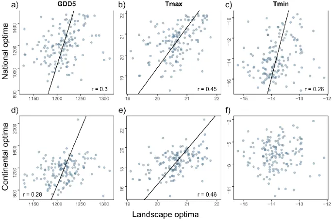
3.1 Correlations between species landscape, national and continental optima 228
Species with higher landscape optima for Tmax also had on average higher national and 229
continental optima (landscape vs national: r = 0.45, P < 0.001; landscape vs continental: r = 230
0.46, P < 0.001, Fig. 2b and e, Appendix 2). For GDD5, there were also positive, albeit 231
weaker, correlations between landscape and national, and landscape and continental optima 232
(landscape vs national: r = 0.30, P < 0.001; landscape vs continental: r = 0.28, P < 0.001, Fig. 233
2b, Appendix 2b). For Tmin, the correlation between landscape and national optima was even 234
weaker (r = 0.26, P = 0.002, Fig. 2c, Appendix 2c), and there was no correlation between 235
landscape and continental optima (r = 0.04, P = 0.65, Fig. 2f, Appendix 2f). 236
237
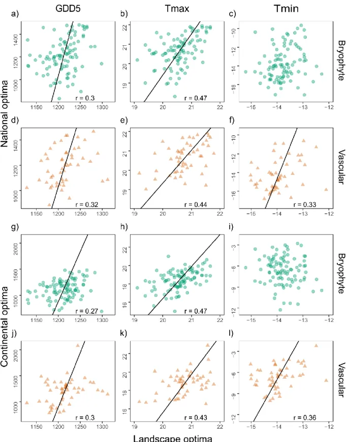
3.2 Differences between bryophytes and vascular plants 238
The relationships between the landscape and national optima and landscape and continental 239
optima for the three temperature variables showed similar patterns for bryophytes and 240
vascular plants in most cases (Fig 3, p>0.05 for the interaction effect, Appendix 3). However, 241
for the model between landscape and continental optima of minimum temperatures there was 242
a significant effect if the interaction between organism group and temperature (Ancova, P = 243
0.0023). For vascular plants, but not for bryophytes, Tmin optima were positively correlated 244
across extents (Fig 3c, f, i and l, Appendix 3). Correlation coefficients did not differ 245
significantly between the two groups, except between Tmin at landscape and continental 246
scales where vascular plants had a higher coefficient than bryophytes (r=0.36 vs. r= –0.13; 247
Fisher r-to-z text, P = 0.004). 248
249
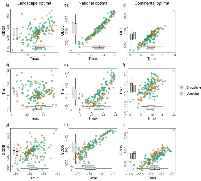
3.3 Within-scale relationships 250
12
There were few differences in the mean optima between the two groups (boxplots in Fig 4). 251
The largest difference was a lower value for growing degree days for bryophytes than for 252
vascular plants in the continental data (P = 0.042, Fig. 4c,i). 253
254
Correlations between the three examined temperature variables differed among the three 255
spatial extents. GDD5 and Tmax were positively correlated at all extents (landscape: r = 0.40, 256
P = 0.005; national: r = 0.89, P < 0.001; and continental: r = 0.83, P < 0.001, Appendix 4 257
and 5), while Tmin was correlated to GDD5 only at the national and continental extents 258
(landscape: r = 0.26, P = 0.07; national: r = 0.91, P < 0.001; continental: r = 0.78, P < 0.001). 259
There were no correlation between Tmin and Tmax at the landscape (r = –0.21, P = 0.15), but 260
a positive correlation at the national and continental extents (national: r = 0.67, P < 0.001; 261
continental: r = 0.39, P < 0.001) (Appendix 4 and 5). 262
263
4. Discussion
264
Our study provided evidence of clear positive correlations between plant species 265
landscape climatic optima and their optima at larger, national and continental extents for two 266
of three examined climate variables. Species growing under locally warm conditions with 267
high maximum temperatures, on average tended to have more equator skewed distributions, 268
and vice versa. In this context the landscape optima can in fact be closer to a species thermal 269
limit for species at their distribution margins, and the broader implication of our results is that 270
knowledge about a species wider geographic distribution can suggest where in a focal 271
landscape it is most likely occurring. At the same time, it is important to note that the highest 272
observed correlation coefficient between landscape and a larger scale optima was 0.47, 273
suggesting that the relationships are relatively weak. Also notable is that the pattern observed 274
for maximum temperature was largely absent for minimum temperature.Few studies have 275
13
specifically tested if it is possible to upscale or downscale distributions across areas of 276
different spatial extents, while the question of upscaling and downscaling distributions in 277
relation to grain size has received more attention (see below). However, the question of up- or 278
downscaling across spatial extent resembles the more investigated question of how well future 279
species distributions can be predicted based on current species distributions (e.g. Austin and 280
Van Niel, 2011; Franklin et al. 2013), and if species niches are consistent across areas (Wasof 281
et al., 2015). However, Kambach et al. (2019) studied different extents and demonstrate that 282
the niche breadth plants in the Alps is a poor predictor of the global niche breadth of the same 283
species. Our results showed that correlations between optima at different spatial extents 284
differed among environmental variables, which suggest that some relationships might be more 285
linked to causal drivers, while others are mostly correlative. Thus, the success of upscaling 286
and downscaling between different spatial extents or predictions of distributions in new areas 287
may sometimes be good and sometimes misleading, depending on whether the identified 288
variables representing causal drivers of distributions (see also Menke et al. 2009). 289
One problem with comparing models at different geographical extents is that the grain 290
size often is larger in larger areas. Larger grid cells fail to detect more of the within grid 291
heterogeneity (Randin et al., 2009, Meineri and Hylander 2017), and as a result different sets 292
of variables, varying over different spatial scales, might explain the distribution at different 293
grain sizes (Pearson and Dawson, 2003; Menke et al., 2009; Connor et al. 2018). However, 294
Collingham et al. (2000) did not find that the influence of different environmental variables 295
varied among grain size, and was optimistic regarding the possibility of upscaling to coarser 296
resolutions, especially when holding the spatial extent constant. In contrast, models calibrated 297
at larger grid cells did not produce realistic downscaled distribution maps for three invasive 298
plant species in Britain, although this might have been partly due to the fact that distributions 299
were not in equilibrium with environmental conditions at either spatial scale (Collingham et 300
14
al., 2000). Still, data from larger grid cells might generate downscaled distribution maps that 301
are quite accurate in some cases, as shown for several species groups in Britain (Barwell et al. 302
2014, Fernandes et al. 2014), and the field is developing fast (Keil et al. 2013, Groom et al. 303
2018). We found very similar patterns when correlating the landscape optima to fine-gridded 304
national data and to coarse-gridded continental scale data. This suggest that our larger scale 305
datasets quite well describe the distributional optima for the species, despite the difference in 306
both extent and grain size. A likely reason for this pattern is that both dataset covers long 307
latitudinal gradients, which are more important to estimate optima than within grid-cell 308
variation. Thus, for studies focusing on niche hypervolume size or shape there is a larger risk 309
for biases due to different grid sizes than in studies focusing on niche centroids (Kambach 310
2019). 311
The correlations between landscape and continental optima were strongest for 312
maximum temperature, weaker but significant for growing degree days, and even weaker or 313
not significant for minimum temperature. Both growing degree days and maximum 314
temperature characterize the climatic conditions during the plant growing season, suggesting 315
that these variables should have an important effect on plant performance. However, 316
minimum temperature has also been highlighted as important for species distributions at 317
different spatial scales (Aschcroft et al., 2011; Dobrowski, 2011; Scherrer and Körner, 2011; 318
Illán et al., 2014), including the range limits of tree species towards cold conditions (Sakai, 319
1979; Körner, 2012, Kreyling et al. 2015). Niche conservatism has been higher for the cold 320
than warm thermal limit for a number of alpine plant species (Pellissier et al., 2013). 321
However, a majority of our studied species might not be affected by yearly minimum 322
temperature in northern regions such as in our focal landscape, since they are resting and 323
protected by snow cover during winter periods there (cf. Vercauteren et al., 2013). Trees and 324
shrubs that extend above the snow cover are more affected by winter frosts than for example 325
15
herbs (Walter and Breckle, 1989). Thus, the correlation between minimum temperature and 326
species landscape scale distribution may not be so informative for continental scale 327
distribution and vice versa when part of the distribution is including winters with snow cover. 328
Yet, perhaps minimum temperatures during late spring, which we did not include in this 329
study, might have a stronger effect on distributions (Muffler et al. 2016). Although both 330
growing degree days and maximum temperature might influence distributions, it is difficult to 331
disentangle their independent effects since they are correlated and correlations are similar at 332
all the scales. In contrast, the correlations between minimum and maximum temperature were 333
in different directions at the different spatial scales; notably even with a tendency to be 334
negatively correlated at the landscape scale (Appendix 4c and f). This difference in 335
correlations among climatic variables between scales may explain why we found less of 336
landscape-large scale optima correlations for minimum temperature than for growing degree 337
days and maximum temperature (Hylander et al., 2015, Meineri et al., 2015). Similarly, 338
Menke et al. (2009) suggested that differences in the distribution of environmental conditions 339
between areas greatly reduces the predictive power of species distribution models 340
parameterized in different areas. Such difference in distribution of environmental conditions 341
might apply also to our case, even if our focal landscape is nested within the other areas, 342
partly explaining different patterns for maximum and minimum temperatures. 343
Several factors may contribute to weak correlations between landscape and larger 344
scale optima. A likely ecological explanation to this is that several factors interact, in a 345
species-specific way, to determine where a species can occur in the landscape (e.g. Gaston, 346
2009, Zellweger et al., 2016). For example, while two species might have similar high 347
continental optima for growing degree days, this might be due to a direct dependence on 348
longer growing season in one of the species but due to dependence on humid conditions, 349
which are correlated with growing degree days, for the other species. As a consequence, they 350
16
might differ in landscape optima for growing degree days if the correlation between growing 351
degree days and humidity is different at the landscape scale than at the continental scale 352
(Hylander et al. 2015). In our study many species, especially of bryophytes, with a high 353
maximum temperature landscape optima also had a low minimum temperature optima at 354
landscape scale (Fig 4d), reflecting the tendency of a negative correlation between these 355
variables in this particular landscape (Appendix 4d). This fact constrains the possibility for 356
strong simultaneous correlations for both maximum and minimum optima between landscape 357
and larger scales optima, since the two variables at larger scales were strongly positively 358
correlated (Appendix 4e and f). Also, local adaptation, biotic interactions and dispersal 359
limitation are likely to decrease the strength of the correlations between spatial scales 360
(Lavergne et al. 2010; Svenning et al. 2015; Herrero et al. 2016). Still, the optima correlations 361
for maximum temperature found in our study lend support to the notion that populations of 362
the same species to some extent are influenced similarly by climatic variables across their 363
geographical range (e.g. Pearman et al., 2008; Wiens et al., 2010; Wasof et al., 2015). Given 364
that many of the species are close to their poleward distribution limit in the focal landscape, 365
we might have expected a clustering of species landscape optima at the warmest end of the 366
climate gradients. Yet, a visual inspection of the graphs does not reveal any such clustering 367
(Fig 2 and 3). The regression slopes and correlation coefficients were overall very similar for 368
vascular plants and bryophytes. This was somewhat surprising given that these groups have 369
quite different ecophysiological traits and it could be expected that the distribution of vascular 370
plants would be mostly influenced by growing degree days while the distribution of 371
bryophytes is more influenced by maximum temperatures, affecting moisture conditions 372
(Dynesius et al. 2009; Gotsch et al. 2017). The reproduction of bryophytes is facilitated by 373
water and the poikilohydric state of bryophytes causes them to easily dry up (Proctor, 2009). 374
In particular, many forest bryophytes are likely to be favoured by moist conditions (Hylander 375
17
et al., 2005; Gotsch et al. 2017). Higher incoming solar radiation, and thus warmer maximum 376
temperature, might lead to shorter periods of net assimilation and reproduction due to drought 377
(Hylander, 2005; Proctor, 2009). This is perhaps the reason for the somewhat colder 378
maximum temperature optima at the landscape scale for bryophytes than for vascular plants 379
(cf. Ratcliffe, 1968). The vascular plants in this study had somewhat higher values of growing 380
degree days at the continental scale compared to bryophytes, which indicate the possible 381
importance of a warm and long growing season for their performance. Yet, the only 382
difference found between vascular plants and bryophyte correlations was a significant 383
correlation of minimum temperature optima between landscape and continental scales for 384
vascular plants that was not detected for bryophytes. Thus, even if most vascular plants are 385
under the snow in the winter it seems like the southern species still to some extent have a 386
higher chance of finding a suitable site in places with mild winter conditions. It would be 387
interesting to find out to what extent there is a stronger co-occurrence pattern of southern 388
vascular plants than southern bryophytes in the rare type of places with a combination of 389
warm long summers and mild winters in the focal landscape. 390
In conclusion, the correlations between landscape optima and optima at larger spatial 391
extents suggest that there is sufficient climatic variation also in topographic heterogeneous 392
landscapes for the distribution of sessile species to be regulated by climate (Scherrer and 393
Körner, 2011; Ashcroft and Gollan, 2012; Meineri et al., 2015). In our study system, optima 394
of maximum temperature had relatively strong correlations between the scales, while optima 395
for minimum temperature were correlated for vascular plants but not bryophytes. We may 396
thus to some extent infer the drivers of distributions of species at larger spatial extents by 397
studying landscape climatic optima, and vice versa. However, the fact that the strength of 398
correlations differed between the three examined temperature variables suggest that it is not 399
possible to routinely upscale or downscale species distributions across geographical extents. 400
18 401
Acknowledgements 402
We would like to thank Johannes Forsberg, Kerstin Kempe, Samuel Olausson and Liselott 403
Wilin for assistance in the field. Benny Willman helped with some data acquisitioning and 404
modelling. Thanks to the County administration board of Västernorrland that provided 405
permission for studies at Halsviksravinen, Omneberget, Skuleberget, Vällingsjö urskog and 406
Älgberget-Björnberget nature reserves, and at Skuleskogen national park. This work was 407
funded by the strategic program Ekoklim and the Bolin Center for Climate Research at 408 Stockholm University. 409 410 Author contributions 411
JD, KH and JE designed the study. JD collected the field data and downloaded most of the 412
data from databases. JD and DMC did the majority of the analyses with supervision from EM. 413
JD wrote the first draft of the ms and all authors contributed to the interpretation of the data, 414
revision of the text and final approval. 415
416
References
417
1. Alberto, F.J., Aitken, S.N., Alia, R., Gonzalez-Martinez, S.C., Hanninen, H., Kremer, A., 418
Lefevre, F., Lenormand, T., Yeaman, S., Whetten, R., Savolainen, O. 2013. Potential 419
for evolutionary responses to climate change evidence from tree populations. Global 420
Change Biology 19, 1645-1661. 421
2. Araújo, M., Thuiller, M., Williams, P.H., Reginster, I. 2005. Downscaling European 422
species atlas distributions to a finer resolution, implications for conservation planning. 423
Global Ecology and Biogeography 14, 17–30. 424
19
3. Azaele, S., Maritan, A., Cornell, S.J., Suweis, S., Banavar, J.R., Gabriel, D., Kunin, W.E. 425
2015. Towards a unified descriptive theory for spatial ecology, predicting biodiversity 426
patterns across spatial scales. Methods in Ecology and Evolution 6, 324-332. 427
4. Aschcroft, M.B., French, K.O., Chisholm, L.A. 2011. An evaluation of environmental 428
factors affecting species distributions. Ecological Modelling 222:24-531. 429
5. Ashcroft, M.B., Gollan J.R. 2012. Fine-resolution (25 m) topoclimatic grids of near-surface 430
(5 cm) extreme temperatures and humidities across various habitats in a large (200 x 431
300 km) and diverse region. International Journal of Climatology 32, 2134–2148. 432
6. Austin M.P., Van Niel K.P. 2011. Improving species distribution models for climate 433
change studies, variable selection and scale. Journal of Biogeography 38, 1–8. 434
7. Barwell, L.J., Azaele, S., Kunin, W.E., Isaac, N.J.B. 2015. Can coarse-grain patterns in 435
insect atlas data predict local occupancy? Diversity and Distributions 20, 895-907. 436
8. Blonder, B. 2018. hypervolume: High Dimensional Geometry and Set Operations Using 437
Kernel Density Estimation, Support Vector Machines, and Convex Hulls. R package 438
version 2.0.11. 439
9. Blonder, B., Morrow, C. B., Maitner, B., Harris, D. J., Lamanna, C., Violle, C., Enquist, B. 440
J., Kerkhoff, A. J. 2017. New approaches for delineating n-dimensional hypervolumes. 441
Methods of Ecology and Evolution 9, 305-319. 442
10. Brown J.H. 1984. On the Relationship between Abundance and Distribution of Species. 443
The American Naturalist 124, 255–279. 444
11. Collingham Y.C., Wadsworth R.A., Huntley B., Hulme P.E. 2000. Predicting the spatial 445
distribution of non-indigenous riparian weeds, issues of spatial scale and extent. 446
Journal of Applied Ecology 37, 13–27. 447
20
12. Connor, T., Hull, V., Vina, A., Shortridge, A., Tang, Y., Zhang, J.D., Wang, F., Liu, J.G. 448
2019. Effects of grain size and niche bredth on species distribution modelling. 449
Ecography 41, 1270-1282. 450
13. Dahlberg C.J., Ehrlén J., Hylander K. 2014. Performance of forest bryophytes with 451
different geographical distributions transplanted across a topographically 452
heterogeneous landscape, PLoS ONE 9, e112943. 453
14. Dobrowski S.Z. 2011. A climatic basis for microrefugia, the influence of terrain on 454
climate. Global Change Biology 17, 1022–1035. 455
15. Dynesius, M., Hylander, K., Nilsson, C. High resilience of bryophyte assemblages in 456
streamside compared to upland forests. Ecology 90, 1042-1054. 457
16. Europe 2014. Continent. Available at, 458
http,//www.britannica.com/EBchecked/topic/195686/Europe [Accessed 29 July 2014] 459
17. Fernandes, R.F., Vicente, J.R., Georges, D., Alves, P., Thuiller, W., Honrado, J.P. 2014. A 460
novel downscaling approach to predict plant invasions and improve local conservation 461
actions. Biological Invastion 16, 2577-2590. 462
18. Franklin J., Davis F.W., Ikegami M., Syphard A.D., Flint L.E., Flint A.L., Hannah L. 463
2013. Modeling plant species distributions under future climates, how fine scale do 464
climate projections need to be? Global Change Biology 19, 473–483. 465
19. Fridley J.D. 2009. Downscaling climate over complex terrain, high finescale < 1000 m. 466
spatial variation of near-ground temperatures in a montane forested landscape (Great 467
Smoky mountains) Journal of Applied Meteorology and Climatology 48, 1033–1049. 468
20. Gaston, K.J. 2009. Geographic range limits, Achieving synthesis. Proceedings of the 469
Royal Society B Biological Sciences 276, 1395–1406. 470
21
21. Gotsch, S.G., Davidson, K., Murray, J.G., Duarte, V.J., Draguljic, D. 2017. Vapor 471
pressure deficit predicts epiphyte abundance across an elevational gradient in a 472
tropical montane region. Americal Journal of Botany 12, 1790-1801. 473
22. Groom, Q.J., Marsh, C.J., Gavish, Y., Kunin, W.E. 2018. How to predict fine resolution 474
occupancy from coarse occupancy data. Methods in Ecology and Evolution 9: 2273-475
2284. 476
23. Guisan A. and Zimmermann N.E. 2000. Predictive habitat distribution models in ecology. 477
Ecological Modelling 135, 147 186. 478
24. Hampe A., Rodríguez-Sánchez F., Dobrowski S., Hu F.S., Gavin D.G. 2013. Climate 479
refugia, from the last glacial maximum to the twenty-first century. New Phytologist 480
197, 16–18. 481
25. Hannah L., Flint L., Syphard A.D., Moritz M.A., Buckley L.B., McCullough I.M. 2014. 482
Fine-grain modeling of species’ response to climate change, holdouts, stepping-stones, 483
and microrefugia. Trends in Ecology and Evolution 29, 390–397. 484
26. Herrero, A. Almaraz, P. Zamora, R., Castro, J., Hodar, J.A. 2016. From the individual to 485
the landscape and back, time-varying effects of climate and herbivory on tree sapling 486
growth at distribution limits. Journal of Ecology 104, 430-442. 487
27. Hess, G.R., Bartel, R.A., Leidner, A.K., Rosenfeld, K.M., Rubino, M.J., Snider, S.B., 488
Rickets, T.H. 2006. Biological Conservation 132: 448-457.Hijmans R.J., Cameron 489
S.E., Parra J.L., Jones P.G., Jarvis A. 2005. Very high resolution interpolated climate 490
surfaces for global land areas. International Journal of Climatology 25, 1965–1978. 491
28. Hurlbert, A.H., White, E.P. 2005. Disparity between range map- and survey-based 492
analyses of species richness: patterns, processes and implications. Ecology Letters 493
8:319-327.Hylander K. 2005. Aspect modifies the magnitude of edge effects on 494
bryophyte growth in boreal forests. Journal of Applied Ecology 42, 518–525. 495
22
29. Hylander K., Dynesius M., Jonsson B.G., Nilsson C. 2005. Substrate form determines the 496
fate of bryophytes in riparian buffer strips. Ecological Applications 15, 674–688. 497
30. Hylander K., Ehrlén J., Luoto M., Meineri E. 2015. Microrefugia, Not for everyone. 498
AMBIO 44, 60–68. 499
31. Illán J.G., Thomas C.D., Jones J.A., Wong W.-K., Shirley S.M., Betts M.G. 2014. 500
Precipitation and winter temperature predict long-term range-scale abundance changes 501
in Western North American birds. Global Change Biology 20, 3351–3364. 502
32. Kambach, S., Lenoir, J., Decocq, G., Welk, E., Seidler, G., Dullinger, S., Gégout, J.-C., 503
Guisan, A., Pauli, H., Svenning, J.-C., Vittoz, P., Wohlgemuth, T., Zimmermann, 504
N.E., Bruelheide, H. 2019. Of niches and distributions: range size increases with niche 505
breadth both globally and regionally but regional estimates poorly relate to global 506
estimates. Ecography 42, 467-477. 507
33. Kreyling, J., Schmid, S., Aas, G. 2015. Cold tolerance of tree species is related to the 508
climate of their native ranges. Journal of Biogeography 42, 156–166. 509
34. Lembrechts, J., Ivan, N., Lenoir, J. 2018. Incorporating microclimate into species 510
distribution models. Ecography 42, 1-13. 511
35. Lenoir J. et al. 2013. Local temperatures inferred from plant communities suggest strong 512
spatial buffering of climate warming across Northern Europe. Global Change Biology 513
19, 1470-1481. 514
36. Lenoir, J. et al. 2017. Climatic microrefugia under anthropogenic climate change, 515
implications for species redistribution. Ecography 40, 253–266. 516
37. Keil, P., Belmaker, J., Wilson, A.M., Unitt, P., Jetz, W. 2013. Downscaling of species 517
distribution models: a hierarchical approach. Methods in Ecology and Evolution 2013: 518
4: 82-94.Keppel, G. et al. 2012. Refugia, identifying and understanding safe havens 519
for biodiversity under climate change. Global Ecol. Biogeogr. 21, 393–404. 520
23
38. Körner C. 2012. Alpine Treelines. Springer, Basel. 521
39. Lavergne S., Mouquet N., Thuiller W., Ronce O. 2010. Biodiversity and climate change, 522
Integrating evolutionary and ecological responses of species and communities.Annual 523
Review of Ecology, Evolution, and Systematics 41, 321–350. 524
40. Mascher J.W. 1990. Ångermanlands flora. SBT-redaktionen, Lund. 525
41. Meineri E., Dahlberg C.J. Hylander K. 2015. Using Gaussian Bayesian networks to 526
disentangle direct and indirect associations between landscape physiography, 527
environmental variables and species distribution. Ecological Modelling 313, 127–136. 528
42. Meineri, E. and Hylander, K. 2017. Fine-grain, large-domain climate models based on 529
climate station and comprehensive topographic information improve microrefugia 530
detection. Ecography 40, 1003–1013. 531
43. Menke, S.B., Holway, D.A., Fisher, R. N., Jetz, W. 2009. Characterizing and predicting 532
species distribution across environments and scales: Argentine ant occurrences in the
533
eye of the beholder. Global Ecology and Biogeography 18:50-63 534
44. Muffler, L., Beierkuhnlein, C., Aas, G., Jentsch, A., Schweiger, A.H., Zohner, C., 535
Kreyling, J. 2016. Distribution ranges and spring phenology explain late frost 536
sensitivity in 170 woody plants from the Northern Hemisphere. Global Ecology and 537
Biogeography 25, 1061-1071. 538
45. Pearman P.B., Guisan A., Broennimann O., Randin C.F. 2008. Niche dynamics in space 539
and time. Trends in Ecology and Evolution 23, 149–158. 540
46. Pearson R.G. and Dawson T.P. 2003. Predicting the impacts of climate change on the 541
distribution of species, are bioclimate envelope models useful? Global Ecology and 542
Biogeography 12, 361–371. 543
47. Peel M.C., Finlayson B.L., McMahon T.A. 2007. Updated world map of the Köppen-544
Geiger climate classification. Hydrology and Earth System Sciences 4, 439–473. 545
24
48. Pellissier L., Bråthen K.A., Vittoz P., Yoccoz N.G., Dubuis A., Meier E.S., Zimmermann 546
N.E., Randin C.F., Thuiller W., Garraud L., Van Es J., Guisan A. 2013. Thermal 547
niches are more conserved at cold than warm limits in arctic-alpine plant species. 548
Global Ecology and Biogeography 22, 933–941. 549
49. Phillips S.J., Anderson R.P., Schapire R.E. 2006. Maximum entropy modeling of species 550
geographic distributions. Ecological Modelling 190, 231–259. 551
50. Proctor M.C.F. 2009. Physiological ecology. Bryophyte Biology ed. by B. Goffinet and J. 552
Shaw., pp. 237–268. Cambridge University Press, New York. 553
51. Proctor M.C.F. 2011. Climatic responses and limits of bryophytes, comparisons and 554
contrasts with vascular plants. Bryophyte Ecology and Climate Change. ed. by Z. 555
Tuba, N.G. Slack, L.R. Stark., pp. 35–54. Cambridge University Press, New York. 556
52. Randin C.F., Engler R., Normand S., Zappa M., Zimmermann N.E., Pearman P.B., Vittoz 557
P., Thuiller W., Guisan A. 2009. Climate change and plant distribution, local models 558
predict high-elevation persistence. Global Change Biology 15, 1557–1569. 559
53. Ratcliffe D.A. 1968. An ecological account of Atlantic bryophytes in the British Isles. 560
New Phytologist 67, 365–439. 561
54. Revelle, W. 2018. psych: Procedures for Personality and Psychological Research, 562
Northwestern University, Evanston, Illinois, USA. R package version 1.8.12. 563
55. R Core Team 2014. R, A language and environment for statistical computing. R 564
Foundation for Statistical Computing, Vienna. 565
56. Sakai A. 1979. Freezing tolerance of evergreen and deciduous broad-leaved trees in Japan 566
with reference to tree regions. Low temperature science. Ser. B, Biological sciences 567
36, 1–19. 568
25
57. Scherrer D. and Körner C. 2011. Topographically controlled thermal-habitat 569
differentiation buffers alpine plant diversity against climate warming. Journal of 570
Biogeography 38, 406–416. 571
58. Svenning JC, Eiserhardt WL, Normand S, Ordonez A, Sandel B 2015.The influence of 572
paleoclimate on present-day patterns in biodiversitv and ecosystems. Annual Review 573
of Ecology, Evolution and Systematics 46, 551-572. 574
59. Swedish Meteorological and Hydrological Institute 2016. Klimatdata. Available at, 575
http,//www.smhi.se/klimatdata [accessed 29 January 2016] 576
60. Synes N.W. and Osborne P.E. 2011. Choice of predictor variables as a source of 577
uncertainty in continental-scale species distribution modelling under climate change. 578
Global Ecology and Biogeography 20, 904–914. 579
61. Thuiller W., Richardson D.M., Pyšek P., Midgley G.F., Hughes G.O., Rouget M. 2005. 580
Niche-based modelling as a tool for predicting the risk of alien plant invasions at a 581
global scale. Global Change Biology 11, 2234–2250. 582
62. Trivedi M.R., Berry P.M., Morecroft M.D., Dawson T.P. 2008. Spatial scale affects 583
bioclimate model projections of climate change impacts on mountain plants. Global 584
Change Biology 14, 1089–1103. 585
63. Ureta, C., Martorell, C., Cuervo-Robayo, A.P., Mandujano, M.A.C., Martinez-Meyer, E. 586
2018. Inferring space from time, On the relationship between demography and 587
environmental suitability in the desert plant O. rastrera. PlosONE 8, e0201543. 588
64. Vercauteren N., Lyon S.W., Destouni G. 2013. Seasonal influence of insolation on fine-589
resolved air temperature variation and snowmelt. Journal of Applied Meteorology and 590
Climatology 53, 323–332. 591
65. Walter H. and Breckle S.-W. 1989. Ecological systems of the geobiosphere, 3 temperate 592
and polar zonobiomes of northern Eurasia. Springer-Verlag, Berlin Heidelberg. 593
26
66. Wasof S., Lenoir J., Aarrestad P.A., et al. 2015. Disjunct populations of European 594
vascular plant species keep the same climatic niches. Global Ecology and 595
Biogeography 24, 1401–1412. 596
67. Wiens J.J., Ackerly D.D., Allen A.P., Anacker B.L., Buckley L.B., Cornell H.V., 597
Damschen E.I., Jonathan Davies T., Grytnes J.-A., Harrison S.P., Hawkins B.A., Holt 598
R.D., McCain C.M., Stephens P.R. 2010. Niche conservatism as an emerging principle 599
in ecology and conservation biology. Ecology Letters 13, 1310–1324. 600
68. Woodward F.I. and Williams B.G. 1987. Climate and plant distribution at global and local 601
scales. Vegetatio 69, 189–197. 602
69. Zellweger, F., Baltensweiler, A., Ginzler, C., Roth, T., Braunisch, V., Bugmann, H., 603
Bollmann, K. 2016. Environmental predictors of species richness in forest landscapes, 604
abiotic factors versus vegetation structure. Journal of Biogeography 43, 1080-1090. 605
606 607
Supplementary material Appendix 1-5. 608
Additional data and R-code deposited at XXX 609
27 Figures
611 612
613
Figure 1 a) Location of the focal landscape with the 49 inventoried sites in the middle of 614
Sweden between the latitudes 62°50’ and 63°12’ N. The national data was for the whole of 615
Sweden (small map in the left of the panel) b) The location of the continental area in Europe. 616
Background overview maps, © Lantmäteriet Gävle 2014 I2014/00691. 617
28
619
620
Figure 2. The correlations between landscape versus national climatic optima (a-c) and 621
landscape versus continental climatic optima (d-f) of all species for the three temperature 622
variables growing degree days GDD5, maximum temperature Tmax °C, and minimum 623
temperature Tmin °C., respectively. A major axis type II regression is projected on significant 624
correlations p<0.05 with corresponding r-values. Note that the ranges on the axes as well as 625
the metrics are different in the different data sets (see methods). 626
29
628 629
630
Figure 3. The correlations between landscape and continental climatic optima of (a-c) 631
bryophytes and (d-f) vascular plants for the three temperature variables growing degree days 632
30
GDD5, maximum temperature Tmax °C and minimum temperature Tmin °C., respectively. 633
Panels (g-l) show the same for correlations between landscape and national climatic optima. 634
A major axis type II regression is projected on significant correlations p<0.05 with 635
corresponding r-values. Note that the ranges on the axes as well as the metrics are different in 636
the different data sets (see methods). 637
31
639
640
Figure 4. Variation in optima of growing degree days GDD5, maximum temperature Tmax 641
°C and minimum temperature Tmin °C within three different scales a-c) landscape, d-f) 642
national and g-i) continental scales. Bryophytes (96 species) are shown with green circles and 643
vascular plants (50 species) with orange triangles. Boxplots indicate the median and variation 644
for the optima of bryophytes grey and vascular plants light grey, where significant differences 645
at P < 0.05 between the two groups are indicated with the symbols a–b. 646