Equilibrium Storage in a Markov Economy
Anna Creti
∗Università Bocconi
Bertrand Villeneuve
†University of Tours
Finance of Energy Markets Laboratory
‡0§September 2007
Abstract
We model an economy that alternates randomly between abun-dance and scarcity episodes. We develop an original method to char-acterize in detail the structure of the Markovian competitive equilib-rium. Accumulation and drainage of stocks are the main focuses. Eco-nomically appealing comparative statics results are proved. We also characterize stationary distribution of states. We extend the model to discuss price stabilization policies, injection and release costs, and limited storage capacity. Overall, the analysis delineates the notion of “flexible economy.”
Keywords.Price stabilization, strategic stocks, supply risk
JEL codes.C61, Q48, L90.
∗Anna Creti, Università Bocconi and IEFE, Via Sarfatti 25, 20136 Milan, Italy. Email:
†Corresponding author. Bertrand Villeneuve, CREST-J320, 15 boulevard Gabriel Péri,
92245 Malakoff cedex, France. Email: [email protected].
‡Joint Laboratory Paris Dauphine University, CREST and EDF R&D.
§This research has benefited of the support of the Chair Dauphine-EDF-Calyon
1
Introduction
Storage models are hard to tackle. Even the simplest specification of the pro-duction and storage technologies leads to intractable equations. Most results involve proving existence and uniqueness of the equilibrium, together with some qualitative properties (prices are monotonic in stock and in storage cost, stockouts happen with positive probability and stocks have an upper limit). As far as simulation based econometrics (GMM estimators as in Deaton and Laroque, 1992, 1996) or the illustration of a theoretical possibility are con-cerned (convenience yield,1 analysis of the Samuelson effect,2 backwardation3 as in Routledge et al, 2000), this is a suitable approach. Our aim is not to extend the existing models but rather to propose a simple case set in con-tinuous time to facilitate the parameterization of shock persistence, and to characterize finely the behavior of the economy.
Our approach is innovative as it does not rely on fixed point methods, but directly constructs the equilibrium, assuming that agents observe the random occurrence of the so-called abundance and scarcity periods. We focus on a Markov economy, so the competitive equilibrium consists of price functions that only depend on the current state. We fully describe the dynamics of accumulation and drainage by means of a system of differential equations. Relying on the phase diagram, we identify a number of economic border con-ditions and prove existence and uniqueness of the equilibrium. Technically, we confront a Boundary Value Problem with conditions imposed on singular points.
In such an equilibrium, stocks are smoothly piled up in an abundance state and smoothly drained in a crisis state. The relationship between the state of the economy (the endogenous stocks and the exogenous random variable) and the price is informative about behavior of the economy. For example, we can see that the upper bound of the stocks is never reached in finite time and we can also evaluate the speed at which stocks are drained out. Besides such qualitative results, we provide comparative statics on the upper bound of the stocks and equilibrium price schedules with respect to all the parameters of the model.
1The notion of convenience yield was introduced by the economists Kaldor and Working
who studied the theory of storage. In the context of commodities, the convenience yield captures the benefit from owning a commodity minus the cost of storing it. The flow of benefits from storage (the reduction in production costs) drives a wedge between the price of a commodity today and its value in the future.
2The Samuelson effect arises when, for a given commodity, forward price volatility
declines with the contract horizon.
3Backwardation occurs when the price of a commodity for the actual period exceeds
Price functions give a logically complete picture of the equilibrium. Nev-ertheless, the characterization of the stationary distribution of states has an intuitive appeal as it directly informs as to where the economy is likely to be. The frequency of stockouts as well as the propensity of the economy to adjust stocks can thus be assessed. The stationary distribution is described by differential equations, which opens up the way to qualitative analysis and comparative statics. The dependency of the shape of the state density to the parameters is addressed.
Our model is motivated by two economic issues placed high on the Euro-pean policy agenda. Storage as determined in response to persistent shocks is instructive for the energy policy debate about the role of gas or petroleum strategic reserves to manage supply disruptions, especially when dependency on foreign resources raises serious concerns. The existing theoretical litera-ture on energy supply security, mostly inspired by the theory of exhaustible resources, considers either the extraction rate of one country when foreign import, though needed to complement national production, can suddenly de-fault,4 or strategic behavior of consuming countries confronting oligopolistic or cartelized supply.5 However useful these analyses may be for the long run, they ignore the question of how to reach any desired stock level and how to deal with uncertainty about the duration of supply disruption. Efficiency loss of recommended policies may be underestimated.
We also shed some light on the banking of CO2 pollution permits, a fi-nancial mechanism whose application is being discussed in the context of the European Trading Scheme, i.e. a market-based approach to environ-mental control. A number of research works have already analyzed the role of uncertainty in emission permit markets, studying in particular the SO2 banking mechanism allowed by the American Clean Air Act. Most results concern optimum individual strategy and not the equilibrium. This limi-tation notwithstanding, several aspects of risk-averse utilities’ are studied.6 4This trade-off has been analyzed by several authors (for example Stiglitz, 1977,
Sweeney, 1977, Hillman and Van Long, 1983, Hugues Hallet, 1984).
5See for instance Nichols and Zeckhauser (1977), Crawford et al (1984), Devarajan and
Weiner (1987), Hogan (1983).
6On the role of banking in smoothing permit prices, see Carlson and Sholtz (1994)
and Godby et al (1997), on its effect on control costs, see Montero (1997). Hennessy and Roosen (1999), Ben-David et al (2000) and Baldursson and von der Fehr (2004) examine the impact of stochastic pollution on production decisions in competitive markets, showing that the existence of uncertainty as to the magnitude of pollution tends to reduce production activities to the situation of non-stochastic pollution with the same mean rate of emissions. Rousse and Sévi (2006) use a methodology similar to the one proposed by the models on precautionary saving with uncertainty on future income. Econometric estimates on US data provide evidence that utilities bank in response to uncertainty, particularly
The study of equilibrium in Schennach (2000) assumes that risk-neutral firms minimize their expected discounted costs. When firms anticipate the possi-bility of a permit stockout, the expected change in marginal abatement costs could be negative. Potential permit stockout could partially explain normal backwardation in permit prices; the same mechanism is at the core of the results in Routledge et al (2000). Our analysis is not focused on financial phenomena, though the model could serve that purpose; this said, we can illustrate the precautionary motive for banking emission rights, when the output market alternates between booms and busts (namely, when electric-ity demand is influenced by unexpected climate constraints) or there is a sudden but temporary increase in input costs.
The economic relevance of our model and its practicality are illustrated by three extensions.
First, we study the impact of a constant price policy. This apparently extreme choice is instructive for both gas and pollution permit markets be-cause a regulatory authority could be tempted to stabilize gas or permit prices around a particular target (or path) of prices. Understanding the mechanisms of equilibrium and comparison with more interventionist policy could serve as a modest guide (or a development thereof) for market design and regulation. In contrast to the previous abundant literature on storage and price stabi-lization,7 results are clear-cut: perfect price stabilization can be reached only if the economy is prepared to let stocks go to infinity. This simple prediction gives a partial answer to doubts as to price stabilization models raised by Williams and Wright (1991), who affirm: “[...] the possible permutations of demand curvature, disturbance structure, initial conditions, supply elasticity and so forth seem nearly infinite. [...] That is the main point: few, if any, general propositions are possible.”
In a second extension of the model, we consider the impact of nonneg-ligible injection and release costs. This better characterizes natural gas or oil storage. Starting from the observation that the commodity is different
when their power is mainly coal-generated.
7Massel (1969), generalizing previous results by Waugh (1944) and Oi (1961), considers
stabilization at exactly the mean price as a decision made to eliminate price fluctuations, presumably enhancing welfare. A costless stock established by an authority achieves the objective and enhances welfare. Welfare analysis of price stabilization has been extended to encompass alternative assumptions about price expectations, risk attitudes (Newbery and Stiglitz, 1981), and nonlinearities (Turnovsky, 1974, 1976, among others). Storage in this literature is made by a public authority, which is in charge of managing a buffer stock. Helmberger and Weaver (1977) is the only model that questions the optimality of stabilization schemes. The private storage industry and arbitrage opportunities are considered, instead, in modern dynamic stochastic models with i.i.d disturbances (Williams and Wright, 1991).
depending on whether it lies outside or inside the reservoir, we show that the results of our analysis are unaffected by this generalization.
Limited storage capacity is also a crucial issue. For instance, gas is often stored in specific natural facilities (such as salt caverns) that are scarce. Also, market rules for emission programmes could impose the use of banking CO2 permits up to a given threshold only. Consistently with the idea of scarcity rent, we show that in the accumulation phase, the price for storage service suddenly jumps above marginal cost when the capacity saturates. Interest-ingly, we find that, in contrast with the unconstrained case, the maximal stock is attained in finite time if the state of abundance is sustained.
The paper is organized as follows. Section 2 sets up the model and section 3 describes the methodology we follow to solve it. Section 4 characterizes the solution qualitatively and quantitatively and proposes comparative statics. Section 5 exposes the statistical properties of the model. Section 6 is devoted to applications and extensions of the model, while Section 7 concludes on the notion of economic flexibility. Proofs are relegated to the Appendix.
2
The model
2.1
Assumptions and parameters
The economy can be in two states, abundance (A) or scarcity (C, for cri-sis). A generic state is denoted σ. Time is continuous and the state changes following conditional Bernoulli processes: the passage from A to C occurs with probability rate λC, and the passage from C to A with probability rate λA. This simple Markov structure captures the fact that regimes have uncertain nature and duration that can be quantified statistically. The un-conditional probabilities of states A and C are, respectively, Pr[A] = λA
λC+λA
and Pr[C] = λC
λC+λA. The ratio λA/λC represent the relative frequencies of
the two states whereas 2(λ−1A + λ−1C )−1 measures the global rate of change.8 Primary production and final demand at a given date are assumed to be nonstrategic (price-taking behavior), they vary with the state and the current price. Consequently, the fundamental data are, for every σ = A, C and every price p, the excess supply functions, i.e. the difference, denoted
8The unconditional rate of change is twice the harmonic mean of the conditional rates
of change
Pr[A] × λC+ Pr[C] × λA=
2 1/λA+ 1/λC
∆σ[p], between production and final consumption.9 These functions measure variations per unit of time, thus conservation of matter imposes that ∆σ[p].dt be the variation of the stocks in a time interval of length dt during which state σ would be sustained.10 These two functions are assumed to be strictly increasing and to have unique, finite, zeros in R+ denoted by p∗σ.These zeros are the prices at which primary production and final consumption would be balanced at each instant, were state σ sustained. To clarify matters, p∗
C > p∗A. Storage is assumed to be competitive and to exhibit constant returns to scale, with carrying costs being the (constant) opportunity cost of capital r and a unit flow cost c (paid per unit of commodity and per unit of time).11 Storers are assumed to be risk-neutral so prices satisfy the following relation-ship
pt+ cdt = (1− rdt)Etpt+dt. (2) The LHS is acquisition price plus stockholding cost over interval dt and the RHS is the expected present value (as for date t) of the stock at date t + dt. Definition 1 A competitive equilibrium is an initial state (C or A and a certain stock) at date 0 (without loss of generality), plus a sequence of prices {pC[S, t], pA[S, t]}t≥0 such that (1) all agents (consumers, producers, storers) are price-takers and form rational expectations; (2) in each state, conserva-tion of matter imposes that current producconserva-tion minus current final consump-tion equals the variaconsump-tion in the stocks.
Definition 2 A Markovian competitive equilibrium is such that the equilib-rium sequence of prices only depends on the current state (σ, S), but neither the date nor the past.
The following focuses on Markovian equilibria, summarized by functions pC[S]and pA[S] (time as an argument can be dropped).
2.2
Fundamental equations
The price functions are necessarily continuous in S over the support of the equilibrium, otherwise the predictable discontinuity would create an
arbi-9These assumptions as similar to those in Deaton and Laroque (1992, 1996) and
Rout-ledge et al (2000). They are consistent with general equilibrium if, for example, infinite horizon consumers have quasi-linear utility (this supposes two goods per period, the stor-able commodity plus a numéraire that could be leisure); the rate of interest is then directly given by the discount rate.
10Shocks can be interpreted as demand or supply shocks. Only the net shock matters. 11The assumption in Deaton and Laroque (1992, 1996) and Routledge et al (2000) is that
a constant fraction of the stock vanishes every period. This type of cost can be included, via a renaming of variables, in r. Our variation is well suited to natural resources.
trage opportunity (e.g. massive buys/sales just before discrete upward/downward jump).
For all S > 0 and a time increment dt, the no-arbitrage equations derived from (2) read
pC[S] + cdt = (1− rdt) ((1 − λAdt)· pC[S + dS] + λAdt· pA[S + dS]),(3) pA[S] + cdt = (1− rdt) ((1 − λCdt)· pA[S + dS] + λCdt· pC[S + dS]).(4) This is a first-order approximation. We let dt converge to 0 and neglect second-order terms, thus (3) and (4) become
∆C[pC]· dpC dS = (r + λA)pC − λApA+ c, (5) ∆A[pA]· dpA dS = (r + λC)pA− λCpC+ c. (6) The boundary value problem basically states that the solution must verify equations (5), (6), pC[0] = p∗C and pA[S∗] = p∗A, where S∗ is the maximum stock. One difficulty is that ∆C[pC[0]] = 0, meaning that
dpC[0]
dS is infinite. Another difficulty is that S∗ is only implicitly defined, its value being de-termined as the point where accumulation stops (pA[S∗] = p∗A implies that ∆A[pA[S∗]] = 0); moreover, at S∗, the RHS of (6) and both factors in the LHS are null, meaning that one condition is imposed at a singular point.
2.3
Summary of the notation
t :time;
σ :generic exogenous state;C : Scarcity/Crisis; A :Abundance;
λC: probability rate that state passes from A toC ; λA: probability rate that state passes from C toA ;
∆σ[p] :excess supply for pricepin stateσ (per unit of time); p∗
σ :zero of∆σ;
S :stocks at a given date;
c :marginal storage cost (per unit of time);
r :riskfree interest rate.
3
The equilibrium
This section establishes that in a Markovian equilibrium, stocks are smoothly piled up in state A and smoothly drained in state C. Moreover, stocks vary between 0 and the upper bound S∗ to be determined, whereas the price is bounded below by p∗
We analyze the system of equations in a phase diagram (pC, pA)in which S is the underlying parameter. This representation facilitates the demon-stration of existence and uniqueness of the equilibrium. Most importantly for economic intuition, it enables qualitative results and comparative statics.
3.1
Phase diagram
Let us define xσ, a function of S, by differential equation x0σ = ∆σ[pσ]· p0σ, with xC[0] = 0 and xA[S∗] = 0. Using this notation in equations (5) and (6), we obtain
x0C = (r + λA)pC − λApA+ c, (7) x0A = −λCpC+ (r + λC)pA+ c. (8) We have an autonomous (S is not in the equations) system of separated variables. We draw the two-dimensional phase diagram with pC ≤ p∗C on the horizontal axis and pA≥ p∗Aon the vertical one. This quadrant is partitioned into three regions, separated by the isoclines where x0C = 0 and x0A = 0 are null, i.e.
(r + λA)pC − λApA+ c = 0and pC ≤ p∗C, pA ≥ p∗A, (CC0) −λCpC+ (r + λC)pA+ c = 0and pC ≤ p∗C, pA ≥ p∗A. (AA0) (CC0)is never empty since by assumption p∗
C > p∗A. (CC0) is above (AA0) in the considered quadrant (see Appendix A.1).
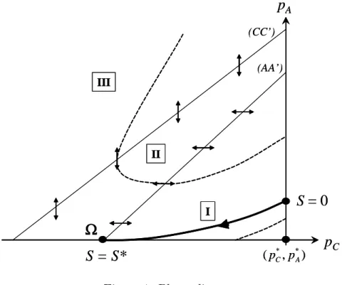
The phase diagram in Figure 1 indicates the shape and relative positions of the trajectories satisfying the motion equations (7) and (8). We define the lowest region, I, as the triangle having (AA0) as a side and (p∗
C, p∗A) as a vertex; the intermediate region, II, lies between the two lines, and the highest region III is above (CC0). In I, p0
C < 0 and p0A < 0; in II, p0C > 0 and p0
A> 0; in III, p0C > 0 and p0A> 0.12
The intersection between (AA0) and horizontal straight line pA = p∗A is especially remarkable. We denote it as Ω = (r+λC
λC p ∗ A+ c λC, p ∗ A).
3.2
Characterization
Proposition 11. In equilibrium, the support of S is an interval [0, S∗]. 12This comes from the facts that in I, x0
C > 0 and x0A < 0; in II, x0C > 0 and x0A> 0;
in III, x0
S = S*
S = 0
I II III (CC’) (AA’)Ω
p
Cp
A * * (pC,pA)S = S*
S = 0
I II III (CC’) (AA’)Ω
p
Cp
A * * (pC,pA)Figure 1: Phase diagram.
2. Stocks are drained during scarcity episodes and accumulated during abundance episodes (∆C[pC[S]]≤ 0 and ∆A[pA[S]]≥ 0 over [0, S∗]). 3. The equilibrium trajectory {(pC[S], pA[S])|S ∈ [0, S∗]} is in region I.
The trajectory starts with pC[0] = p∗C and stops at (pC[S∗], pA[S∗]) = Ω. 4. There is storage in equilibrium (i.e. S∗ > 0) if and only if
(r + λC)p∗A+ c < λCp∗C. 5. The equilibrium is unique
The overall behavior of the prices in equilibrium can be summarized as follows: the unique equilibrium trajectory is necessarily in I, S varies in the interval [0, S∗) and p
A[S] > p∗A and pC[S] < p∗C for S > 0 and S < S∗, and pA[S] and pC[S] decrease with respect to the level of the stock.
Figure 1 shows the shape of the equilibrium trajectory. The condition for positive storage (r+λC)p∗A+c < λCp∗C has a precise economic meaning: crises have to be sufficiently likely and/or sufficiently marked to justify storage. If this condition were not satisfied, there would be no stocks in equilibrium: the price would alternate back and forth between p∗
state C. To avoid this uninteresting case, we assume that the condition for positive storage is satisfied.
3.3
Computations
Numerically, the argument used in the proof of Proposition 1 (point 5) has an extremely useful implication: any starting point close to Ω is on a trajectory that is closer to the equilibrium as we go to the right (i.e. as S decreases) in the phase diagram. In other terms, we can control the maximum error on prices at the starting point (close to Ω) given that the system of equations is self-correcting as S decreases.
Moreover, the system of equations (7, 8) is autonomous, so leaving aside boundary conditions, we know that if (pC[S], pA[S]) follows the equilibrium trajectory for S ∈ [S, S], so does (pC[S + θ], xA[p + θ]) for S ∈ [S − θ, S − θ] where θ is an arbitrary real.
We can now suggest the following algorithm. Algorithm 1 (Trajectory)
1. Fix arbitrarily the upper bound at some arbitrary value S.
2. Choose ε > 0 as small as needed. Consider the trajectory through (pC[S] = r+λλCCp∗A+
c
λC, pA[S] = p
∗
A+ ε), a point above Ω.
3. Solve the differential equations numerically and find the stock S < S such that pC[S] = p∗C.
4. Shift the calculated functions pC and pA to the left by an amount S; S∗
ε = S− S approximates the upper bound S∗.
The error is controlled by ε (a uniform bound on the error). Remark that along a trajectory, dS dpC = ∆C[pC] (r + λA)pC − λApA+ c (9) is well defined over the range of pC i.e. [r+λλCCp∗A +
c λC, p
∗
C] (trajectory is bounded away from (CC0)). Thus we can calculate S∗ as accurately as desired by computing: Sε∗ = Z p∗ C r+λC λC p∗A+ c λC ∆C[pC] (r + λA)pC − λApA+ c dpC. (10)
4
Behavior of the economy
4.1
Comparative statics
In the absence of an explicit expression of price functions and S∗, the com-parative statics relies on exploitation of the phase diagram.
Proposition 2 (Comparative statics) For all S in the support, and for all states σ = C, A ∂p∗ σ[S] ∂c < 0; ∂p∗ σ[S] ∂r < 0; ∂p∗ σ[S] ∂λA < 0; ∂p ∗ σ[S] ∂λC > 0. (11) and consequently ∂S∗ ∂c < 0; ∂S∗ ∂r < 0; ∂S∗ ∂λA < 0; ∂S ∗ ∂λC > 0. (12)
The interpretations are straightforward. An increase in the unit storage costs discourages accumulation, thus at any level of the stocks, the value of the commodity is smaller. Storers will tend to pile up stocks more slowly in abundance, and to run them down faster during crisis. Also, rarer crises diminish the expected yield from storing, to the same effect. This logic has direct consequences on the comparative statics of the limit stock: the value S∗, defined as the solution to equation p∗
A[S] = p∗A, must decrease if function p∗A[S] is diminished.
Linear case. The effects of varying excess supply functions are intricate if we do not restrict the analysis to a specific parametric family. For example, in the noteworthy case of linear excess supply functions, precise results can be found.
Proposition 3 (Linear case) Assume that
∆σ[pσ] = βσ(pσ − p∗σ) with βσ > 0 and p∗σ > 0. (13) 1. For all S in the support and all states σ = C, A
∂p∗ σ[S] ∂p∗ C > 0;∂p ∗ σ[S] ∂p∗ A > 0;∂p ∗ σ[S] ∂βC > 0; ∂p∗ σ[S] ∂βA < 0. (14) and consequently ∂S∗ ∂p∗ C > 0; ∂S ∗ ∂βC > 0; ∂S ∗ ∂βA < 0. (15) The sign of ∂S∂p∗∗ A is ambiguous.
2. As a function of βC and βA, p∗
σ[S] and consequently S∗ are homogeneous of degree 1.
It is plain that a bigger p∗
C should increase the value of storage, hence the effect on prices and maximum stocks. In contrast, a bigger p∗
A has two effects: on the one hand, it increases the price at which stocks are built and thus prices in crisis have to increase altogether to motivate positive holding; on the other hand, the range of prices tightens, meaning that potential gains from the occurrence of a crisis could vanish at smaller values of S. This explains the ambiguity of the impact of p∗
A on S∗.
A higher parameter βC means that a given release has a less depressing effect on the price. In other terms, the profitability of storing in view of releasing at high price when state C arises is better warranted. This gives incentives to store more. A higher parameter βAimplies that building stocks is easier, since piling up has a lesser inflationary effect on the price, hence the negative effect on the equilibrium price. The second point of the proposition illustrates that the first effect dominates when βC and βA are increased in the same proportion.
4.2
Approximate price functions
To better describe the behavior of the economy, we clarify the properties of the equilibrium when stocks are almost empty or close to their maximum. We see in particular how stocks are drained down and why the maximum stocks are not attained in finite time.
Draining out the stock. At S = 0, x0
C is finite and different from 0 (see equation 7); more precisely, xC[S] ∼
0 KCS with KC = (r + λA)p ∗
C + c− λApA[0] > 0. This implies (see Appendix A.5) that
pC[S]− p∗C ∼0 − s 2KC ∆0 C[p∗C] S1/2 (16)
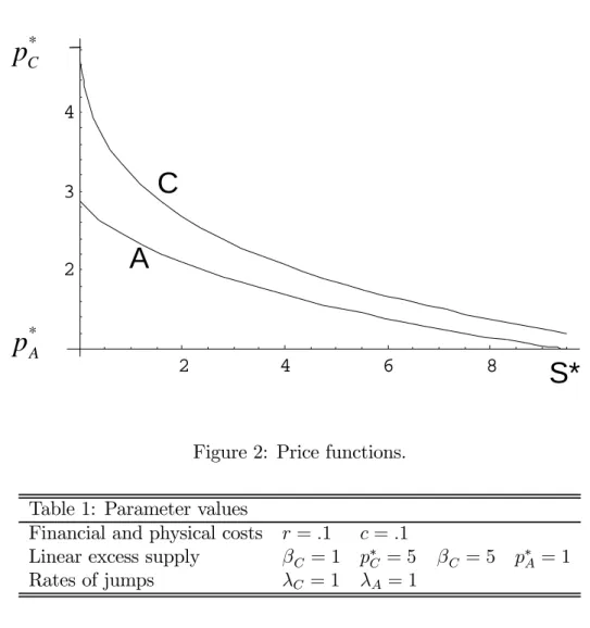
pC is vertically tangent at 0 (Figure 2). As a consequence, if the economy stays in crisis, the complete drainage of the stocks happens in finite time. To show this, it suffices to integrate in a neighborhood of 0 the differential equation
dS
dt = ∆C[pC[S[t]]], (17)
where the RHS can be replaced by its approximation. As long as the economy stays in crisis, starting–without loss of generality–with S0 at date 0, the
integration of equation (17) yields S(t)' Ã p S0− r ∆0 C[p∗C]KC 2 t !2 . (18)
Drainage exhibits smooth landing: the limit of the rate of withdrawal is zero; but drainage time is finite. It is approximately
T0 ' s 2S0 ∆0 C[p∗C]KC . (19)
This implies that the economy is protected only twice as long when stocks are quadrupled.
The comparative statics on KC is based on (11) in Proposition 2. We have ∂KC
∂λC < 0, meaning quite naturally, that a larger propensity to return to the
scarcity state slows down drainage (precaution). Also, ∂KC
∂c > 0 and ∂KC
∂r > 0, meaning that higher storage costs accelerate drainage for given stocks. Remark that ∂KC ∂λA = (p ∗ C−pA[0])−λA ∂p∗ A[0]
∂λA > 0 :a higher propensity to return
to abundance also accelerates drainage (preservation value is diminished). Replenishing. The upper bound S∗ corresponds, as we noticed in sub-section 3.2, to a singular point. The calculation of an approximate solution requires several steps. We show in the Appendix A.5 that xA[S]−xA[S∗]∼S∗
K2
A(S− S∗)2, where KA is a non-negative real number. This implies that pA has a negative finite non-null derivative at S∗ (Figure 2):
pA[S]− p∗A ∼S∗ KA(S− S∗). (20) Even if the economy stays in a state of abundance, the upper bound S∗ is never reached in finite time. The reasoning reminds us of Zeno’s classical paradox, Achilles and the Tortoise. As pA covers half its difference with the limit p∗
A, the variation rate of the stock per unit of time, namely ∆A, is ap-proximately halved (linear approximation of excess demand at p∗
A), meaning that the convergence speed dS/dt is approximately halved. This implies that, whatever the proximity of the target, the duration to cover half the distance to the target is approximately constant, thus the target is never attained. Example. Using the algorithm of subsection 3.3, we solve numerically the system with the parameters in Table 1. The time unit could be the year. We find approximately S∗ ' 9.5. See Figure 2.
2 4 6 8 2 3 4 * C
p
* Ap
S*
A
C
Figure 2: Price functions. Table 1: Parameter values
Financial and physical costs r = .1 c = .1
Linear excess supply βC = 1 p∗C = 5 βC = 5 p∗A= 1
Rates of jumps λC = 1 λA= 1
5
Stock statistics
A state is described by the stock S and the conjuncture (C or A). All states S ∈ [0, S0]with S0 < S∗ are crossed in finite time with probability 1: starting from an arbitrary state, it is easy to find a history (or a set of histories) that leads to another arbitrary state in finite time, this history being associated with positive probability (it suffices to have a long enough accumulation followed by a long enough drainage, or the other way around). Since the equilibrium is Markovian, this property guarantees that there is a unique stationary distribution. This section is essentially devoted to the analysis of this stationary distribution.
5.1
Dynamics
The statistical evolution of the system over time when we observe perfectly the state at a given date is covered in Appendix A.6.
A feature of the model is that in the long run initial information loses relevance. Interior states (i.e. values of S different from 0 and S∗) are just crossed as accumulation or drainage goes on; boundary states, if reached, remain in force until a downward or upward jump occurs. Thus, in the long run, S = 0 and S = S∗ are associated with probabilities whereas values in between are associated with densities.
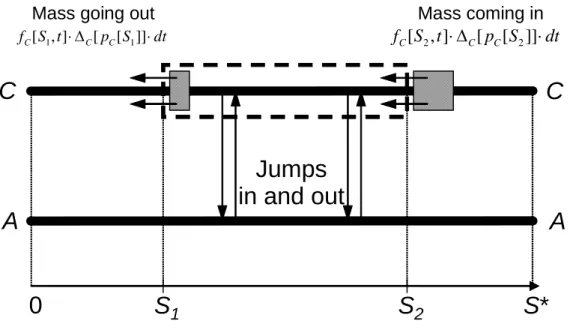
Densities. Assume that, for interior values of the stock S ∈ (0, S∗), a density fσ[S, t] (with σ = C, A) represents the information we have on the system. Take σ = C to fix ideas. Choose S1 and S2 (0 < S1 < S2 < S∗) two levels of the stocks. By definition
Pr[C, S ∈[S1, S2], t] = Z S2 S1 fC[S, t]dS. (21) This gives d Pr[C, S ∈ [S1, S2], t] dt = fC[S1, t]· ∆C[pC[S1]]− fC[S2, t]· ∆C[pC[S2]] +λC Z S2 S1 fA[S, t]dS− λA Z S2 S1 fC[S, t]dS, (22) where the first two terms represent the endogenous evolution of the stocks if the economy remains in crisis, and the third and fourth terms represent the exogenous jumps in and out of the segment due to state changes. Figure 3 illustrates this probability balance.
To find the dynamics of the density, we make S2 converge toward S1 to get dfC[S, t] dt =− d dS(fC[S, t]· ∆C[pC[S]]) + λCfA[S, t]− λAfC[S, t]. (23) Similarly dfA[S, t] dt =− d dS (fA[S, t]· ∆A[pA[S]]) + λAfC[S, t]− λCfA[S, t]. (24)
C
A
0
S*
Jumps
in and out
Mass going out
S
1S
2A
C
1 1 [ , ] [ [ ]] C C C f S t ⋅ Δ p S ⋅dt Mass coming in 2 2 [ , ] [ [ ]] C C C f S t ⋅ Δ p S ⋅dtFigure 3: Probability balance between t and t + dt.
Probabilities. States S = 0 or S∗ are associated with probabilities. We have13
d Pr[C, 0, t]
dt =−λAPr[C, 0]− limS→0(fC[S, t]· ∆C[pC[S]]) , (25) where the first-term represents jumps out (jumps in are negligible since Pr[A, 0, t] = 0 : due to accumulation, this state is left as soon as attained), and the second term represents the depletion of the last remaining stock.
Similarly, d Pr[A, S∗, t] dt =−λCPr[A, S ∗] + lim S→S∗(fA[S, t]· ∆A[pA[S]]) . (26)
5.2
Stationary distribution
The study of stationary distribution can use directly the preceding analysis. We denote the stationary densities by fσ∗[S]for all S ∈ (0, S∗).Define φC[S]≡ f∗
C[S]· ∆C[pC[S]] and φA[S]≡ fA∗[S]· ∆A[pA[S]] (density flows). Dropping the time-dependency factor, and replacing the rates of variation of the stocks by their equilibrium values, equations (23,24) become the system of ordinary
13This expression can be derived from (22) with S
differential equations dφA dS = λAf ∗ C− λCfA∗, (27) −dφdSC = λAfC∗ − λCfA∗. (28) We also have from (25,26)
Pr[0] = 1 λA lim S→0φC, (29) Pr[S∗] = 1 λC lim S→S∗φA. (30) Remark that −φC[S] = φA[S]. (31)
Indeed, consider the open system {(C, s), (A, s)|s ∈ [0, S]} , this equation states that, in a stationary distribution, density flows in (at S for state C) equal flows out (at S for state A). Jumps do not matter since they happen within the system.
Equations (27) and (28) collapse to: dφA dS =− µ λA ∆C[pC[S]] + λC ∆A[pA[S]] ¶ φA. (32)
This first order ordinary differential equation is well defined for S ∈ ]0, S∗[ and can be solved numerically. The Cauchy-Lipschitz theorem is applicable. Algorithm 2 (Stationary distribution)
1. Calculate equilibrium prices pC[S] and pA[S].
2. Fix arbitrarily φ[S] as an initial condition for some S ∈ (0, S∗). 3. Solve numerically the differential equation (32) over ]0, S∗[. 4. Calculate conditional densities fA∗ and fC∗.
5. Calculate the integrals over ]0, S∗[ of f∗
A and fC∗.
6. Remark that Pr[S∗] = 0. Use step 5 to calculate the residual Pr[0] using the facts that Pr[C] = λA/(λC + λA) and Pr[A] = λC/(λC + λA). 7. Normalize f∗
Step 3 must be analyzed in detail. Indeed, ∆C[pC[0]] = ∆C[p∗C] = 0 and ∆A[pA[S∗]] = ∆A[p∗A] = 0, meaning that φ might diverge in such a way that normalization is impossible (integrals at step 5 could diverge). In fact, we check in Appendix A.7, that
Z S∗ 0 fC∗[S]dS <∞ and Z S∗ 0 fA∗[S]dS < ∞. (33) Remark also that the integrals in step 5 can be calculated as accurately as needed, implying that the residual for Pr[0] in step 6 can be computed with the same accuracy.14
The numerical analysis gives instructive results on the overall behavior of the economy. How frequent are stockouts, i.e. how much is Pr[S = 0] compared to Pr[C](= λC
λC+λA)? Is the economy often close to having maximum
stocks or is S∗ a practically unapproachable limit? The last question can be addressed theoretically by characterizing the shape of the density of the stationary equilibrium around S∗.Here we can identify which are the critical parameters that determine the regime of the economy.
Figure 4 shows the stationary densities for the parameters in Table 1. We find Pr[0] = .1, Pr[S∗] = 0.In fact lim
S→0fC = +∞, but fC is approximately proportional at 0 to 1/√S, meaning that the probability of C remains finite (see equation 29). This high density around 0 comes from the fact that the rate of consumption of the stocks decreases steeply as S approaches zero. The high density on the left of S∗ is explained by the fact that accumulation slows down as the stock approaches S∗(see equations (18,19) about drainage speed and time).
In contrast to 0, S∗ is never attained, as we mentioned in Subsection 4.2. Nevertheless, as Proposition 4 shows, the probability mass can be quite concentrated, under precise circumstances, in the neighborhood of the max-imum. Proposition 4 Let KS∗ = √ 2λC (r+λC)2+4∆0A[p∗A]λCM −r−λC (34) with M = [(r+λA)(r+λC)−λAλC]p∗A+(r+λA+λC)c −λC∆C[r+λCλC p∗A+ c λC] > 0. (35) At S∗, f
C is of the order of (S∗− S)KS∗ and fA is of the order of (S∗− S)KS∗−1.
14The alternative method would be to use property (29); however, the numerical
A
2 4 6 8 0.05 0.1 0.15 0.2C
A
S*
Figure 4: Densities. Consequently,1. If KS∗ < 1 : fA increases and diverges as S → S∗. Though the maxi-mum is never attained, any neighborhood of S∗ has a positive proba-bility.
2. If 1 < KS∗ < 2 : fA converges to 0 at S∗ with vertical negative slope. The system is close to the maximum with a positive probability. 3. If KS∗ > 2 : fAconverges to 0 at S∗ with a null slope. The economy is
almost surely far from the upper bound.
Given the discontinuous nature of the comparative statics, singular cases with either KS∗ = 1 or KS∗ = 2 would require higher order approximations
than the one used in Appendix A.8 to be described.
The understanding of the conditions above is relatively complex since all the fundamental parameters play a role. In particular, no simple comparative statics with respect to r or λC emerge. In contrast, the effects of c, λA are obvious ∂KS∗ ∂c < 0; ∂KS∗ ∂λA < 0. (36)
In the linear case, where in particular ∆0
A[p∗A] = βA, we have ∂KS∗ ∂βC > 0; ∂KS∗ ∂βA < 0; ∂KS∗ ∂p∗ C < 0;∂KS∗ ∂p∗ A < 0. (37)
The comparative statics on KS∗, together with the ones on S∗ exposed in
the comments of Proposition 2, outline a notion of flexibility: the higher KS∗,
the less flexible the economy is. Excess supply functions measure the response of prices to given variations in stocks. Small maximum stocks correspond to flexible economies for which large storage would be useless, and accordingly the economy has, statistically, enough time to approach this modest target during abundance period. On the contrary, large maximum stocks mean that the economy with seize (almost) any opportunity to accumulate, which happens in economies where building stocks is a costly process. Accordingly, it is very likely that the random alternation between abundance and scarcity episodes will keep the economy far from the bliss point.
6
Applications and extensions
In this Section, we extend the model by assessing the impact of three kinds of constraints: politically imposed bounds on prices, nonnegligible injection and release costs and limited storage capacity.
Analyzing the impact of a constant price on the dynamic system allows a comparison of the results with those proposed by the abundant literature on stabilization. Following on from this, we show that nonnegligible injection and release fees can be modelled as parallel shifts in the functions pA[S]and pC[S].The main results of our analysis are unaffected by this generalization. Finally, assuming that storage capacity is exogenously constrained, we show that in the accumulation phase, the maximal stock is attained in finite time. Moreover, the price for storage service suddenly jumps above marginal cost when capacity saturates.
6.1
Stabilization, storage and persistent crises
Assume that a central authority imposes a constant price p∗.A price below p∗ A would not be sustainable in the long run (stock will be drained out shortly). A price above p∗
C would cause never ending accumulation, which would be uneconomical. So, the relevant policies consider p∗
A < p∗ < p∗C. Remark that if we preclude rationing, the policy is not strictly applicable since the price must turn to p∗
C when stocks are empty in state C. With rationing, the price may remain formally at p∗,but the marginal shadow value of the commodity would be p∗C anyway.
for stationary distribution. We can solve (32), i.e. dφA dS =− µ λA ∆C + λC ∆A ¶ φA for all S > 0, (38) where λA ∆C+ λC
∆A here is a constant (with a constant price, ∆C < 0and ∆A > 0
are constant). Define p∗ as the solution to the equation λ
A∆A[p]+λC∆C[p] = 0. If p∗ < p∗, then λA ∆C + λC ∆A > 0 ⇔ λA∆A + λC∆C < 0 : on average,
the economy draws on the stocks. This implies that φA is decreasing and the density is a decreasing exponential: lower stocks are more likely. The distribution has an unbounded support, empty stocks in crisis is an event of positive probability during which the price is p∗
C. If p∗ > p∗, then λA
∆C +
λC
∆A < 0 ⇔ λA∆A+ λC∆C > 0 : on average, the
economy piles up stocks. This implies that φA is increasing unboundedly with respect to S. Higher stocks being increasingly likely, normalization is impossible; in other words there is no well defined stationary distribution. Stocks diverge to infinity with probability one and stabilization, in this sense, succeeds.
The case p∗ = p∗ is intriguing. The economy has no tendency to pile up nor to drain out stocks. All positive levels of the stocks are equally likely (the stationary density is flat), meaning that the behavior of the system in the long run is unpredictable.
Stabilization should not be understood in the narrow sense of averaging the price that would be observed in the absence of storage capabilities. Re-mark indeed that p∗,which is the critical threshold, could be higher or lower than the average no-storage price λA
λA+λCp ∗ A+ λC λA+λCp ∗
C.This depends on the sensitivity of excess supply functions to price variations.
The conclusion is straightforward: perfect price stabilization can be reached only if the economy is prepared to let stocks go to infinity. The analysis above is easily extended to the case of limited storage capacity. Any upper bound on stocks leaves positive probability on empty stocks. In that case, the prob-abilities of full storages and stockouts depends on the policy p∗ chosen.
6.2
Injection and release costs
Denote unit injection cost by i and unit release cost by s. Assume that in each state σ = A, C, and for any stocks level S, there are markets for the gas outside and inside the reservoir, the prices being respectively pσ[S] and pI
σ[S]. The (competitive) market equilibrium between outside and inside gases implies that, whenever S > 0,
The structure of the system of equations is preserved, with pI
σ replacing pσ. No arbitrage conditions read
∆C[pIC + s]· dpI C dS = (r + λA)p I C − λApIA+ c, (40) ∆A[pIA− i] · dpI A dS = (r + λC)p I A− λCpIC + c. (41)
Remark that the excess supply functions are shifted, thus boundary condi-tions are
pIC[0] = p∗C − s, (42)
pIA[S∗] = p∗A+ i. (43)
The range of pI
σ is narrower than that of pσ : the minimum is higher, the maximum is lower. As a result, the condition ensuring that there is storage in equilibrium is more restrictive than the one in Proposition 1 (Point 4), i.e. in the linear case
p∗C− s > µ r + λ λC ¶ (p∗A+ i) + c λC . (44)
The phase diagram enables us to show that S∗ is decreasing with respect to the cost parameters s and i. The rest of the comparative statics is identical.
6.3
Limited storage capacity
If the total storage capacity S exceeds S∗,then the unconstrained trajectory remains sustainable; else, rational storers anticipate that boundary condi-tions are modified.
As long as some capacity is vacant, then storage price per unit of gas (per unit of time) remains equal to marginal cost c; the system of equations is exactly the same as the one without any constraint, so the equilibrium is described by a trajectory in region I of the phase diagram. Trajectories below the unconstrained equilibrium start on the vertical axis at a given price for S = 0 and stop on the horizontal axis on the right of Ω for a maximum stock which is smaller than S∗. There is a unique trajectory such that this maximum stock equals exactly S. It describes the unique equilibrium with limited storage capacity. See for example the dashed trajectory below the bold one in Figure 1.
In the accumulation phase, the price for storage service suddenly jumps above marginal cost when capacity is saturated. We denote it by πA.15 Given 15In case of crisis, the stock immediately starts being used so that state (C, S = S)
does not last. This implies that πC, the price of storage services for congestion during the
that pA[S] = p∗A, the no-arbitrage argument in state (A, S = S) can be expressed
λC(pC[S]− p∗A) = rp∗A+ πA. (45) The LHS measures the potential profit from holding stocks and the RHS the cost. Given that pC[S] > r+λλCCp∗A+
c
λC (the terminal point is on the right of
Ω in Figure 1), we have πA> c.
In contrast to the unconstrained case, the maximal stock is attained in finite time if abundance lasts long enough. This explains that the jump in the price of storage services (a discontinuity) is consistent with a continuous price function pA[S] (continuity is necessary for no-arbitrage): before the capacity is full, the price pA[S]decrease steadily; storers incur non-negligible capital losses if the state does not change; this depreciation term does not converge to zero as the maximal stocks are reached; this term is relayed by cost πA> 0 when the constraint becomes binding.
7
Conclusion
Our model has fully described the behavior of a Markov economy in which storage dynamics are determined by random occurrence of crises. Overall, we have proposed the quite appealing notion of “flexible economy”. We have proved that in equilibrium, a more flexible economy (i.e. better able to absorb shocks via production and consumption changes), is less keen to build up large stocks and is much more likely (in terms of probability) to hold maximum stocks. If the reluctance to build large stocks is intuitive, since overall, the value of stocks (or the convenience yield) decreases when an economy can promptly react to a shock, release dynamics are less intuitive. We show that flexible economies go fast towards maximum stocks and just stay there until a shock leads to fast drainage, while inflexible economies incur permanent movement of their stocks, and over a wider interval. This relationship between flexibility and maximum stocks is a result of interest. On this ground, it could be argued that security of supply policies for energy or banking rules for emission rights, which are never neutral with respect to the market equilibrium, should not be set equally across European states, inasmuch as their capabilities to repond to shocks is heterogeneous.
References
[1] Baldursson, Fridrik M.; von der Fehr, Nils-Henrik (2004): “Price Volatility and Risk Exposure: On Market-based Environmental Policy Instruments,”
Journal of Environmental Economics and Management, 48, 682-704.
[2] Ben-David, Shau; Brookshire, David ; Burness, Michael; McKee, Stuart; Schmidt, Christian (2000): “Attitudes Toward Risk and Compliance in Emis-sion Permit Market,” Land Economics, 76, 590-600.
[3] Carlson, Dale A; Sholtz, Anne M. (1994): “Designing Pollution Market In-struments: A Case of Uncertainty,” Contemporary Economic Policy, 12, 114-125.
[4] Chambers, Marcus J.; Bailey, Roy E. (1996): “A Theory of Commodity Price Fluctuations,” Journal of Political Economy, 104, 924-957.
[5] Chaton, Corinne; Creti, Anna; Villeneuve, Bertrand (2005): Gas Storage and Security of Supply, LERNA Working Paper.
[6] Crawford, Vincent; Sobel, Paul Joel; Takahashi, Ichiro (1984): “Bargain-ing, Strategic Reserves, and International Trade in Exhaustible Resources,” American Journal of Agricultural Economics, 66, 472-80.
[7] Deaton, Angus; Laroque, Guy (1992): “On the Behaviour of Commodity Prices,” Review of Economic Studies, 59, 1-23.
[8] Deaton, Angus; Laroque, Guy (1996): “Competitive Storage and Commodity Price Dynamics,” Journal of Political Economy, 104, 896-923.
[9] Devarajan, Shantayanan; Weiner; Robert J. (1989): “Dynamic Policy Coor-dination: Stockpiling for Energy Security,” Journal of Environmental Eco-nomics and Management, 16, 9-22.
[10] Edward, Robert; Hallwood, Charles P. (1980): “The Determination of Opti-mum Buffer Stock Intervention Rules,” Quarterly Journal of Economics, 94, 156—166.
[11] Helmberger, Peter; Weaver, Rob (1977): “Welfare Implications of Commodity Storage Under Uncertainty,” American Journal of Agricultural Economics, 59, 639—651
[12] Hennessy, David. A.; Roosen, Jutta (1999): “Stochastic Pollution, Permits and Merger Incentives,” Journal of Environmental Economics and Manage-ment, 37, 211-232.
[13] Hillman, Arye L.; Van Long, Ngo (1983): “Pricing and Depletion of an Ex-haustible Resource when There is Anticipation of Trade Disruption,” Quar-terly Journal of Economics, 98, 215-233.
[14] Hogan, William (1983): “Oil Stockpiling: Help Thy Neighbor,” Energy Jour-nal, 4, 49-71.
[15] Hughes Hallett, A.J. (1984): “Optimal Stockpiling in a High-Risk Commodity Market: The Case of Copper,” Journal of Economic Dynamics and Control, 8, 211-38.
[16] Massel, Benton (1961): “Price Stabilization and Welfare,” Quarterly Journal of Economics, 83, 284—298.
[17] Montero, Juan P. (1997): “Marketable Pollution Permits with Uncertainty and Transactions Costs,” Resource and Energy Economics, 20, 27-50.
[18] Newbery, David; Stiglitz, Joseph E. (1981): The Theory of Commodity Price Stabilization, Oxford University Press.
[19] Nichols, Albert; Zeckhauser, Richard (1977): “Stockpiling Strategies and Car-tel Prices,” Bell Journal of Economics, 8, 66-96
[20] Oi, Walter (1961): “The Desirability of Price Instability Under Perfect Com-petition,” Econometrica, 29, 58—64.
[21] Rousse, Olivier; Sévi, Benoît (2006): “Banking Behavior under Uncertainty: Evidence from the US Sulfur Dioxide Emissions Allowance Trading Program,” Cahier CREDEN 06.02.63, Université de Montpellier.
[22] Routledge, Bryan R.; Seppi, Duane J.; Spatt, Chester S. (2000): “Equilibrium Forward Curves for Commodities,” Journal of Finance, 55, 1297-1338.
[23] Schennach, Susanne M. (2000): “The Economics of Pollution Permit Banking in the Context of Title IV of the 1990 Clean Air Act Amendments,” Journal of Environmental Economics and Management, 40, 189-210.
[24] Stiglitz, Joseph (1977): “An Economic Analysis of the Conservation of De-pletable Natural Resources,” Draft Report, IEA, Section III.
[25] Sweeney, John (1977): “Economics of Depletable Resources: Market Forces and Intertemporal Bias,” Review of Economic Studies, 44, 125-142.
[26] Turnovsky Stephen, J. (1974): “Price Expectations and the Welfare Gains from Price Stabilization,” American Journal of Agricultural Economics, 56, 706—716.
[27] Turnovsky Stephen, J. (1976): “The Distribution of Welfare gains from Price Stabilization: the case of Multiplicative Disturbances,” International Eco-nomic Review, 17, 133—148.
[28] Waugh, Frederic V. (1944): “Does the Consumer Benefit from price Instabil-ity?” Quarterly Journal of Economics, 53, 602—614
[29] Williams, Jeffrey C.; Wright, Brian D. (1991): “Storage and Commodity Markets,” Cambridge University Press.
A
Appendix
A.1
Phase diagramCompared to (AA0), (CC0) cuts the horizontal axis with a smaller value ofp C. It
suffices to inject pA= p∗A in both equations and to check that λA r + λA p∗A− c r + λA < r + λC λC p∗A+ c λC . (46) This is obvious.
To show that (CC0) cuts the vertical axis with a larger value ofpAthan (AA0),
we inject pC = p∗C into both equations and check that the following equation
remains true (obvious)
r + λA λA p∗C+ c λA > λC r + λC p∗C − c r + λC . (47)
A.2
Proof of Proposition 11. and 2. Price functions are continuous and the stocks vary continuously with respect to time, thus the support of stocks is necessarily an interval.
Assume that over some intervalJ of stocks, ∆C[pC[S]]≥ 0and ∆A[pA[S]]≥ 0 (accumulation only) or ∆C[pC[S]] ≤ 0 and ∆A[pA[S]] ≤ 0 (drainage only).
Clearly, intervalJ can be traversed once at most in history. Consequently, interval
J cannot be part of the equilibrium support of the stocks.
If over some interval, ∆C[pC[S]] ≥ 0 (i.e. pC[S] ≥ p∗C) and ∆A[pA[S]] ≤ 0
(i.e. pA[S]≤ p∗A), accumulation during crises is motivated only by the fact that
the price is expected to rise if the economy stays in crisis (an episode of abun-dance causes a negative shock on the price). This means that dp∗
C[S]/dS > 0.
In consequence, the price in state C is unbounded as well as the support of S, since any length for an episode of scarcity has positive probability to be exceeded.
Such a bubble is unreasonable since it would imply unbounded storage capacity (a transversality condition would translate this common sense remark into mathe-matical language). These arguments show that ∆C[pC[S]]≤ 0(i.e. pC[S]≤ p∗C)
Remark now that if the lower bound of the support were strictly positive, this would mean that a certain quantity of the commodity would be permanently frozen. Denote this level by Smin. Necessarily, pC[Smin] = p∗C, meaning that if
the economy stays in crisis for a long time (a possible event), storers have to pay storage costs without compensation in potential price movements. Consequently, support is bounded below by 0 (Smin = 0).
3. If pC[0] < p∗C, final demand would exceed production for S = 0, which
is impossible with empty storages. This proves that the trajectory starts on the vertical axis (pC[0] = p∗C).
Assume that there is an ε > 0 such that pA stays larger than p∗A+ ε as S
increases. Given the phase diagram, pA reaches its minimum on the straight line
(AA0), if the trajectory starts in I. In any case, as S increases, the trajectory enters in II, then in III, implying that pA overshoots r+λλ A
A p
∗
C +λcA (intersection
between (CC0) and vertical axis). In other terms, for any large enough S, p A
overshoots p∗C while pC remains below pC∗.Thus, as S continues to grow, x0A/x0C
remains finite whether or not pA tends towards infinity. We conclude that any
trajectory in III reaches the vertical axis pC = p∗C for a finite value of the stock.
At this point, drainage stops in state C, but accumulation continues in state A
(xA> 0)), meaning that the stock is never going to be used in the future, which
is uneconomical (see point 1 in this proof).
We conclude from the contradiction that accumulation must stop in stateAfor some stocks S∗;thus necessarilyp
A[S∗] = p∗A.Remark that this can only happen
in I on the horizontal axis at point Ω. 4. From (AA0), we have (r + λC)pA[S∗]− λCpC[S∗] + c = 0 (48) i.e. pC[S∗] = r + λC λC p∗A+ c λC (49) This corresponds to Ω = (r+λC λC p ∗ A+ c λC, p ∗
A).For this intersection to exist, i.e. for
I not to be empty, a sufficient and necessary condition is
(r + λC)p∗A+ c ≤ λCp∗C. (50)
5. We show that there is a unique trajectory passing throughΩ.The Cauchy-Lipschitz Theorem cannot be applied since the system is singular at Ω. We use the following argument: choose any starting point in the interior of I, denoted by
(p0
C, p0A);it is necessarily nonsingular. The trajectory passing through this point is
unique (Cauchy-Lipschitz). Consider the point(p0C, p0A+ ε)whereε is some small
through (p0
C, p0A+ ε), which is positive, decreases asε increases. One can directly
reason on dpA/dpC=∆C[pC] ∆A[pA]· (r + λC)pA− λCpC + c (r + λA)pC − λApA+ c . (51)
This means that trajectories move apart as S increases, i.e. as they approach Ω.
The consequence is that there cannot be multiple trajectories through Ω. This proves existence and uniqueness.
A.3
Proof of Proposition 2We first determine how trajectories move in the phase diagram as parameters change. Rewrite the system of ODE in compact for as
p0C = PC(pC, pA, c, r, λA, λC) or simply PC ( > 0 in region I), (52) p0A = PA(pC, pA, c, r, λA, λC) or simply PA ( < 0 in region I). (53)
Note that ∂PC
∂c = 1/∆C[pC] < 0and ∂PA
∂c = 1/∆A[pA] > 0,thusp0A/p0C = PA/PC
decreases ascincreases (all trajectories in I are flatter). Similar observations prove that all trajectories in I are also flatter when r increases, when λA increases and
when λC decreases.
We can now position equilibrium trajectories as parameters change. Increasing
c orr, or decreasing λC,move Ωto the right; increasing λA has not effect on Ω.
In all cases, the equilibrium trajectory moves below the former one: to eachpC is
associated a smallerpA. Remark that dpdS C = 1/PC < 0,thus S =− Z p∗ C pC[S] dpC PC
(summation along the equilibrium trajectory). (54)
SinceΩgoes to the right ascincreases, the range ofpC becomes smaller; it remains
to be verified that 1/PC,as a function ofpC,is also smaller. For example, along
the equilibrium trajectories, for a fixed pC dPC dc = 1 ∆C[pC] | {z } − +∂pA ∂c |{z} − ×∂P∂pC A |{z} + < 0. (55)
(PC grows in absolute value and thus 1/PC decreases in absolute value.) This
proves that as c increases, a given price is associated with a smaller S. Similar reasonings can be applied to the other parameters to prove the claims.
A.4
Proof of Proposition 3 We have PC = (r + λA)pC − λApA+ c βC(pC− p∗C) , (56) PA = (r + λC)pA− λCpC+ c βA(pA− p∗A) . (57)Clearly, trajectories in I are steeper with a higher βC or a smaller βA. Remark that the frontier of I (Ω in particular) is unchanged in this comparative statics. Remark also (this concerns point 2) that a proportional increase of βC and βA
does not change the trajectories (but a given point corresponds to a different S).
The type of reasoning used in the proof of Proposition 2 can now be applied to show the claims.
The comparative statics with respect top∗
C andp∗Arequire further precautions.
In the former, remark that trajectories are steeper with a higher p∗
C (pC < p∗C)
and that I is extended to the right (trajectories are simply going further to the right). These two effects concur to increase the price for given stocks. In the latter, trajectories are flatter with a (say) smaller p∗
A but Ω moves along down (AA0).The first effect decreases prices, hence point 1, but the second could lead
to a higher S∗ (a smaller function is integrated over a longer interval, since the
range of pC increases, see equation 54).
A.5
Equivalent expressions for prices On the right of 0. We havexC[S] =
Z pC[S]
p∗ C
∆C[p]dp, (58)
thus, writing first-order approximation on both sides we get
KCS + o(S) = 1 2∆ 0 C[p∗C](pC[S]− p∗C) 2+ o(p C[S]− p∗C) 2, (59) which yields pC[S]− p∗C ∼0 − s 2KC ∆0 C[p∗C] S1/2. (60)
On the left ofS∗. Given that, according to (7),p0
C[S∗]6= 0,we can approximate pC[S]aroundS∗ withpC[S∗] + p0C[S∗](S− S∗) + o(S− S∗).We denote p0C[S∗]
by −M, with M =−[(r+λA)(r+λC)−λAλC]p∗A+(r+λA+λC)c λC∆C[r+λCλC p∗A+ c λC] > 0. (61) Given that xA[S] = Z p∗A pA[S] ∆A[p]dp, (62)
we can calculate that pA[S]− p∗A+ o(pA[S]− p∗A) = q 2 ∆0 A[p∗A]x 1/2 A [S],or equiva-lently pA[S]− p∗A= q 2 ∆0 A[p∗A]x 1/2 A [S] + o(x 1/2 A [S]).
We plug these two equivalent expressions into (8), which yields
x0A= (r + λC) s 2 ∆0 A[p∗A] x1/2A + λCM (S− S∗) + o(S− S∗) + o(x 1/2 A ), (63)
Consider now the ODE
y0 = (r + λC) s 2 ∆0 A[p∗A] y1/2+ λCM (S− S∗) with y[S∗] = 0. (64)
The unique solution to (64) is KA2(S∗− S)2 with KA=
√(r+λ
C)2+4∆0A[p∗A]λCM −r−λC
2∆0
A[p∗A] . (65)
We show now that this exact solution of approximate ODE (64) is an approxima-tion of the soluapproxima-tion to ODE (63).
Consider the residualo(S− S∗) + o(x1/2A [S]) in the ODE (63). For allε > 0, there is a left neighborhood ofS∗, denoted V
ε, in which the absolute value of the
residual is smaller thanε× (S∗− S)and ε× (x1/2
A [S]). Consider the ODE y0 = " (r + λC) s 2 ∆0 A[p∗A] + ε # y1/2+(λCM−ε)(S−S∗) with y[S∗] = 0. (66)
The solution to this equation is smaller than xA on Vε : indeed, both x0A and y0
are negative, but if y > xA for some S in Vε, it remains so for any larger stock
because y0 > x0A. This is in contradiction with the fact that y[S∗] = xA[S∗]. In
other terms, xA[S]≥ ⎡ ⎣ r (r+λC+ q βA 2 ε)2+4βA(λCM −ε)−r−λC− q βA 2 ε 2βA ⎤ ⎦ 2 (S∗− S)2. (67)
A similar reasoning shows that xA[S]≤ ⎡ ⎣ r (r+λC− q βA 2 ε) 2+4β A(λCM +ε)−r−λC+ q βA 2 ε 2βA ⎤ ⎦ 2 (S∗− S)2. (68)
These two inequalities give the approximation of xA atS∗.
A.6
Statistical evolution from a known stateTo fix ideas, denote the observed state at, say, date t = 0,by conjuncture A and stocks S0.Conditionally on staying in stateA,the probability mass (initially 1) is
attached to a unique level of the stocks; but this mass itself is eroded by potential jumps. Other states (except 0 and S∗)are associated with a density, as we shall
develop now.
The mass point Smax[t] (where the index max recalls that the support of the
distribution is bounded above by this time dependent value) evolves following
dSmax
dt = ∆A[pA[Smax]] > 0 with Smax[0] = S0, (69)
whereas the lower bound of the distribution follows
dSmin
dt = ∆C[pC[Smin]] < 0 until 0 is reached, with Smax[0] = S0. (70)
Both values move deterministically. Clearly,
Pr[A, Smax[t], t] = e−λCt, (71)
which is the probability that no crisis has ever happened since date 0.
States inside the interval [Smin[t], Smax[t]] are associated with a positive
den-sity; outside the interval, density is null. States (C, 0, t) and (A, Smax[t], t) are
mass points (the former only after some time has elapsed, so thatSminhas reached
0).
To fully characterize the statistical evolution from a known state, we prove the following preliminary lemma that explains how a pointwise probability becomes a density. Lemma 1 lim S→Smax[t] fC[S, t] =− λCe−λCt ∆C[pC[Smax[t]]] + ∆A[pA[Smax[t]]] , (72)
Proof. Consider states {(C, S)|S ∈ [Smax[t]− dS, Smax[t]]} withdS small.
To calculate the probability of this event at date t, we have to trace back histories that lead to these states.
Denote dtand dSA the unique time interval and stock variation such that a
jump from (A, Smax[t]− dSA) to(C, Smax[t]− dSA)at date t− dt followed by
drainage between datet− dtand t has led to state (C, Smax[t]− dS).
Clearly, all the jumps happening from the current mass point between dates
t− dt and t (and only these), give states in [Smax[t]− dS, Smax[t]] at date t.16
So a first-order approximation of the probability we seek is the probability that a jump from {(A, S)|S ∈ [Smax[t]− dSA, Smax[t]]} to C has taken place between
date t− dt and t.This probability is λCe−λCtdt, thus Pr[{(C, S)|S ∈ [Smax[t]− dS, Smax[t]]}] =
λCexp[−λCt]dt
dS . (73)
We have to calculate the relationship between dSC, dSA,and dt. From the stock
dynamics we have dt = dS− dSA ∆C[pC[Smax[t]]] = dSA ∆A[pA[Smax[t]]] . (74)
The middle term is the time needed, given drainage speed, to pass from stocks
Smax[t]− dSA to stocks Smax[t]− dS. The RHS is the time needed, given
ac-cumulation speed, to pass from Smax[t]− dSA to Smax[t]. After straightforward
substitutions, we let dS go to 0 and prove the result.
We are now equipped with a complete set of equations to describe the dynamics. Indeed, (72) and (23,24) can be used to describe statistically the system over time. The exercise is numerically demanding.
A.7
Proof of convergence of Algorithm 2 Remark that the ODE commanding φA can be writtenφ0A φA =− µ λA ∆C + λC ∆A ¶ . (75)
On the right of S = 0, ∆C → 0 so the RHS of (75) is equivalent to −∆λA
C, i.e.,
using (16), to √K0
S where K0 is a nonnegative real K0 = λA ∆0 C[p∗C] √ KC . (76)
16Given the small size of the interval, we can neglect histories involving two
jumps, so relevant histories can only consist of one jump from state A and some drainage.
Thus limS→0φAis finite and strictly positive. Indeed, for all ε > 0,there exists
η such that for allS ≤ η,
(1− ε)√K0 S ≤ φ0A φA ≤ (1 + ε) K0 √ S. (77)
Take S1 and S2 both smaller than η with S1 ≤ S2 and integrate the inequality
above between these two reals. We find
2(1− ε)K0( p S2 − p S1)≤ ln φA[S2] φA[S1] ≤ 2(1 + ε)K 0( p S2− p S1). (78)
This proves that φA is bounded away from 0 (fix S2 and let S1 converge to 0).
Given that φA is also monotonic (increasing) in a neighborhood of 0, the limit
that we denote byφA[0]exists and is nonnegative.
So, at 0, fA is finite and nonnegative whereas fC ∼0 KfC
√
S whereKfC is some
nonnegative real. This implies that, though the density fC diverges at 0, its
integral is well defined.
A.8
Proof of Proposition 4 On the left of S∗, ∆A → 0 so the RHS of (75) is equivalent to −∆λC
A, i.e.
KS∗
S−S∗
where KS∗ is a nonnegative real with
KS∗ =
λC βAKA
. (79)
For allε > 0,there existsη such that for allS ≥ S∗− η, (1− ε) KS∗ S∗− S ≤ − φ0A φA ≤ (1 + ε) KS∗ S∗− S. (80)
TakeS1andS2 both larger thanS∗−ηwithS1 ≤ S2 and integrate the inequality
between these two real numbers. We find
−(1 − ε)KS∗ln S∗− S 2 S∗− S1 ≤ − ln φA[S2] φA[S1] ≤ −(1 + ε)K S∗ln S∗− S 2 S∗− S1, (81) i.e. ∙ S∗− S2 S∗− S1 ¸(1+ε)KS∗ ≤ φφA[S2] A[S1] ≤ ∙ S∗− S2 S∗− S1 ¸(1−ε)KS∗ . (82)
This implies that limS→S∗φA= 0, from which we can conclude thatPr[S∗] = 0.
We can now derive a tight condition on the shape of the density functionfA
around the upper boundS∗. Indeed, given thatφA= fA· ∆A, fA[S]is proportional to(S∗−S)
KS∗−1. (83)