COMPARISON OF DATA TRANSFER METHODS
BETWEEN TWO DIFFERENT MESHES.
P. Bussetta∗
and J-P. Ponthot∗ ∗
LTAS MN2L, Aerospace & Mechanical Engineering Department, B52/3, Universit´e de Li`ege
Chemin des Chevreuils, 1; B-4000 Liege, Belgium
Key words: Data Transfer Method, Weak Form, Mortar Element, Finite Element, Finite Volume
Abstract. Many problems solved with the finite element method require more than one mesh (i.e. one specific mesh for each Physic or a remeshing is needed). The Data Transfer Method used, has a great importance in the capacity to solve the problem and in the reliability of the solution. In general, the data is composed of two kinds of fields (defined thanks to the nodal values or at the integration points). In this paper, the more used Data Transfer Method is compared with the Data Transfer Methods based on a Weak Form (using Mortar Element or Finite Volume).
1 Introduction
The numerical resolution with the Finite Elements Method of many multi-physical problems require more than one mesh. On the one hand, some problems require one specific mesh for each Physic (i.e. one mesh for the mechanical part and another one for the thermal part). On the other hand, in some cases, during the computation a remeshing is needed. In all these cases, the Data Transfer Method used to transfer information from one mesh to another has a great importance in the capacity to solve the problem and in the reliability of the solution. In general, two kinds of fields have to be transferred: the first is defined thanks to the nodal values (primary field) and the second one is defined at the integration points (secondary field). Currently, despite the research effort, no Transfer Method has been recognized as the best. Each method has important disadvantages.
This paper compares the more used Data Transfer Method (Element Transfer Method [1, 2]) with the Data Transfer Methods based on the Weak Form (using Mortar Element [3, 4] or Finite Volume [5, 6, 7]).
2 Definition of the problem
In this paper a problem is computed with the finite element method. During the computation, a Data Transfer is needed from the mesh call old mesh to the one call new mesh. Some primary and secondary fields known on the old mesh are needed on the new mesh. The field P is known on the old mesh thanks to the primary field Pold. The old
mesh is composed of nold
e elements, noldn nodes and the nodal values of Pold is noted P•old.
The value of Pold on each element eold is written as:
Pold= nelem n X j=1 Nj.Pjold (1)
where Nj is the shape function of the node j in the element eold and nelemn the number
of node of the element. The field S is estimated on the old mesh by the secondary field Sold. The value of Sold on each element eold is defined by means of the value at the
integration points (noted •S
old). The fields P and S are evaluated on the new mesh
thanks to the primary field Pnew and the secondary field Snew, respectively. The aim
of the Data Transfer Method is to define on the new mesh, the nodal values of Pnew
(Pnew
• ) and the value at the integration points of S new (
•S
new). The properties of the
Data Transfer Method should be: • weak numerical diffusion, • conservation of the extrema, • easily treatment of the boundaries. 3 Transfer Methods
The Data Transfer Method makes the link between the two discretisations. The re-liability of the field on the new mesh is directly linked with the Data Transfer Method used.
3.1 Element Transfer Method
The Element Transfer Method (ETM) is the most commonly used. The computation of the field on the new mesh is done in two steps:
• Firstly, for each characteristic point (node or integration point) of the new mesh a search is done to find the element of the old mesh eold in which the characteristic
point lies inside.
• For the secondary field Sold, the nodal values of the element eold(eS•old) are computed
by extrapolation of the values at the integration points of this element (•S
old). So,
value of the field on this characteristic point is computed by interpolation of the nodal values of the element eold ([1, 2]), as:
P•new = nelem n X j=1 Nj.Pjold= P old (x) (2) or : •S new = nelem n X j=1 Nj.eSjold (3)
This method does not deal with the elements of the new mesh. These elements have no influence on the value of the field. The transfer is done from the old mesh to a characteristic point of the new mesh. On the one hand, for the secondary field, this method does not conserve the extrema because of the extrapolation on the nodal values. On the other hand, the extrema are conserved for the primary field, but due to geometrical approximations, some nodes on the boundary can be outside of the old mesh. So, a special treatment is required for the boundaries.
3.2 Mortar Element Transfer Method
The Mortar Element Transfer Method (METM) is based on a weak conservation form of the field (using Mortar Element [3]). The field on the new mesh are not directly computed at the characteristic points. But, it is evaluated considering that the integral of the difference between the value of the fields on the new mesh and the value on the old mesh is null ([3, 4, 8]). This integral is done over the new mesh. To compute this integral, for each element, the nodal values of the secondary field (Sold or Snew) are defined (in
function of the values at the integration points of the element). The nodal values are noted eSold
• for an element of the old mesh and eSnew
• for an element of the new mesh.
The value of these fields on each element is defined like the primary field (see equation 1, but in the general case, these nodal values are different for each element). The value of the primary field Pnew on the new mesh is done thanks to the relation:
nnew e X enew =1 Z enew (Pnew− Pold)f de = 0 (4)
and the relation between the secondary field Snew and Sold is defined for each element
enew of the new mesh by:
Z
enew
(Snew− Sold)f de = 0 (5)
where f is a weighting function defined on each element enew (like a primary field). The
The transfer relation of the secondary field (equation (5)) can be written like: nnew n X A=1 nnew n X B=1 NAB1 (e new )SBnew− NA2(e new , Sold) ! = 0. (6) Where N1
AB(enew) and NAC2 (enew, Sold) are the mortar elements linked with the element
enew defined as:
NAB1 (enew) = Z enew NANB de NAC2 (e new, Sold) = Z enew NASoldde (7)
where Niis the shape function of node i (A or B) in the element enew. NAC2 is the coupling
term.
The transfer relation of the primary field (equation (4)) can be written like:
nnew n X A=1 nnew n X B=1 NAB1 Pnew B − nold n X C=1 NAC2 Pold C fA= 0. (8) Where N1
AB and NAC2 are the mortar elements defined as:
NAB1 = nnew e X enew=1 NAB1 (enew) N2 AC = nnew e X enew=1 NA2(enew, N C) (9)
where NC is the shape functions of the node C in the corresponding element eold.
3.2.1 Computation of mortar element The first Mortar Element (N1
AB) is computed by numerical integration over the element
of the new mesh enew (because is a product of two shape functions of this element). The
evaluation of the coupling term (the second Mortar Element, N2
A(enew, •)) is more complex.
Because, in the general case, the field Sold is not continue on each element of the new
mesh. In addition, the sum of the shape functions Nold
C on each element of the old mesh
is not a polynomial function on each element of the new mesh (enew). A numerical and
an exact integration are used to compute this Mortar Element.
Numerical integration The mortar element is computed by numerical integration over each element of the new mesh. For the element of the new mesh enew, the computation
is done with nip integration points. The numerical integration supposes that the value of
the field on the old mesh can be evaluated by a polynomial function on each element of the new mesh.
Exact integration Each element enew of the new mesh is divided in nsub
e elements, as
each sub-element (esub) is only over one element of the old mesh. So, on each element
esub, Nold
C is a polynomial function. Finally, the mortar element is computed exactly by
numerical integration over each sub-element esub (because is an integration of polynomial
function). The exact integration of mortar element considers all intersections between the element of the new mesh and the elements of the old mesh. However, with the numerical integration, the mortar elements are evaluated in function of the intersection in which the integration point lies inside. So, the intersections than are smaller than the influence area of the integration point can be ignored.
3.2.2 Evaluation of the field on the new mesh
Global solving (GS) The relation between the nodal value of the field Snew on each
element of the new mesh and the value of the field Sold (equation (6)) can be written as:
N1 11(enew) · · · N1n1 elem n (e new) ... . .. ... N1 nelem n 1(e new ) · · · N1 nelem n n elem n (e new) Snew 1 ... Snew nelem n = N2 1(enew, Sold) ... N2 nelem n (e new, Sold) (10)
The size of this equation is equal to the number of node of the element of the new mesh. The value at each integration point is equal to the interpolation of the nodal values. This equation can be solved for each element of the new mesh.
For the primary field, the equation (8) can be written as: N1 11 · · · N1n1 new n .. . . .. ... N1 nnew n 1 · · · N 1 nnew n n new n Tnew 1 ... Tnew nnew n = Pnold C=1N1C2 TCold .. . Pnoldn C=1Nn2new n CT old C (11)
The size of this equation is equal to the number of node of the new mesh. In addition, the solution of this equation cannot certify the conservation of the extrema.
Local solving (LS) To obtain a local system, a diagonal matrix is used. The value of the diagonal term is equal to the sum of the line (or the column, because the matrix is symmetric). This is totally equivalent to the row-sum technique used to lump mass matrix in explicit time integration method.
So the value of the field S on each node of the element enew is done by:
Snew A = N2 A(enew, Sold) Pnelemn B=1 NAB1 (enew) (12) The value at each integration point of the element enew is computed by interpolation of
And, the value of the field P on each node is done by: PAnew= Pnoldn C=1NAC2 PCold Pnnewn B=1 NAB1 (13) With this method, the weak conservation of the field is done in a cell composed of the elements of the new mesh including the node A. This technique increases the area of com-putation of nodal value and in the same time the numerical diffusion. But, in opposition of the global solving, the local solving conserves the extrema.
To sum up, the evaluation of the field is done at the node of the new mesh on a function of the shape function of the elements of the new mesh and the value of the field on the elements of the old mesh.
3.3 Finite Volume Transfer Method
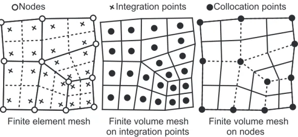
With the Finite Volume Transfer Method (FVTM), each field is rebuild thanks to a finite volume mesh (called old finite volume mesh on the old finite element mesh and new finite volume mesh on the new finite element mesh). The finite volumes are called cells. For the primary field, the cells are based on the node of the finite elements (see figure 1). On the finite volume mesh build for a secondary field, the cells are based on the integration points of the elements of the finite element mesh (see figure 1). So, each field is transferred from one old finite volume mesh to a new finite volume mesh. The same procedure is used to transfer the primary and the secondary field (to more information see [5]).
Figure 1: Finite element mesh and finite volume mesh based on integration points and on the nodes
The value of the field ϕnew (primary or secondary) on one cell is equal to the value of
element mesh. The value of the of ϕnew on one cell cnew of the new finite volume mesh (ϕnew • ) is done by: ϕnewcnew = R cnewϕ olddc Vnew c . (14)
Where ϕold is the value of the field on the old finite volume mesh. Like with the mortar
element, a numerical or an exact integration can be used to evaluate the coupling between the cells of the old and the new mesh.
Numerical integration The value of the field ϕnew on the cell cnew is defined by
numerical integration over this cell. This computation supposes that the field on the old finite volume mesh can be evaluated by a polynomial function on this cell.
Exact integration A super-mesh is built, each cell cnew of the new mesh is divided in
nc
sub cells, like each of them corresponds only to one cell of the old mesh. For each cell
cnew the value of ϕnew
cnew is done by:
ϕnewcnew = Pn c sub csub=1Vcsub× ϕ old cold Vnew c . (15) Where ϕold
cold is the value of the cell of the old mesh corresponding to the sub-cell c
sub. V csub
is the value of the volume (the surface in two dimensions) of the sub-cell csub. The exact
integration of coupling considers all intersections between the cell of the new mesh and the cells of the old mesh.
4 Examples
The difference between these Data Transfer Methods is shown on two dimensional academic examples. These examples expose the numerical diffusion and the evaluation of the data on the boundaries. The meshes are composed of quadrilateral elements. The evaluation of the Mortar Element N1
AB is done by numerical integration using two Gauss
points in each direction. For the numerical integration, the coupling elements (Mortar Element N2
AC or coupling between cells) are evaluated with five Gauss points in each
direction. For the exact integration, the evaluation of the coupling elements is done using six Gauss points on each triangle of the subdivision (to exact integration of quadratic function). These two examples are be used to compare the transfer of a primary field with the Transfer Element Method and the Transfer with Mortar Element in [9].
4.1 Numerical diffusion
The numerical diffusion lies to the Data Transfer Operator is studied with this example. A primary and a secondary field are known on the square. The square’s sides are meshed by 30 elements. A rotation of π/8 is apply on this square. The Data is transferred from
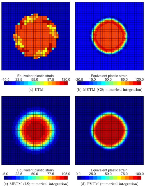
the moved mesh to the initial mesh. The initial value of the field is of a hundred inside a circle and null outside. The centre of the circle is identical to the centre of the square and the radius is the half of the side’s square.
(a) ETM (b) METM (GS; numerical integration)
(c) METM (LS; numerical integration) (d) FVTM (numerical integration)
The comparison of the numerical diffusion is done after twenty transfers (see figures 2(a), 2(b), 2(c) and 2(d)). These figures show that the numerical diffusion is minimized with the METM with global solving and the FVTM (the both with numerical computation of coupling terms). But the METM with global solving does not conserve the extrema, this Transfer Method introduces oscillations around a steep variation (see figure 2(b)). In this case, the difference between the numerical and the exact integration of coupling terms is not significant.
4.2 Influence of boundaries
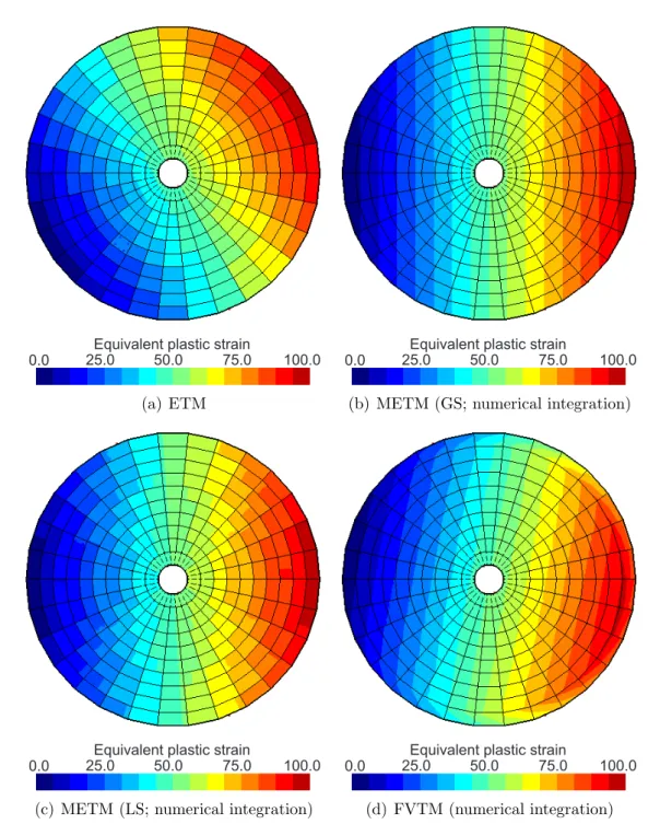
To study the influence of the boundaries, a mesh of a disc with a hole is used. Like the first problem, the transfer is done after rotation of π/8 from the moved mesh to the initial mesh. The half circle is divided in fifteen elements and the radius in ten. The exact value of the field is a linear function of the abscissa (from zero to hundred). The difficulty is that in the general case, the nodes on the boundaries of the new mesh are not inside an element of the old mesh.
Figures 3 show the value of the field after sixteen transfers (one revolution). This problem proves that the ETM applied to a primary field requires a special technique to deal with the boundaries. The nodes located on the boundaries of the new mesh do not lie inside any element of the old mesh. This problem does not appear with the transfer of a secondary field (see figures 3), because the computation of the field is done on the integration points of the new mesh and these points generally lie inside of an element of the old mesh. In addition, the computation of the coupling terms by numerical integration does not consider the part of the elements that is outside of the other mesh. This explains that the METM with global solving does not introduce any error after the transfer (see figure 3(b)). The error after the transfer with the other Transfer Methods is a numerical diffusion and not a wrong evaluation of the field on the boundaries (see figures 3(c), 3(a) and 3(d)). The exact integration of the coupling terms introduces an error of space discretisation of the boundaries. The parts of the element of the old mesh that do not lie inside any element of the new mesh are not considered on the Mortar Elements. In the same time, the parts of the element of the new mesh that do not lie inside any element of the old mesh are considered and the value of the field inside is null. So, the integral of the field over the new mesh is not equal to the integral over the old mesh. This error impairs the quality of the solution.
(a) ETM (b) METM (GS; numerical integration)
(c) METM (LS; numerical integration) (d) FVTM (numerical integration)
Figure 3: Numerical diffusion after sixteen transfers of the secondary field (4 Gauss points)
5 Conclusion and future works
In conclusion, this paper presents a comparison of Data Transfer Methods between two different meshes. The Data Transfer Methods based on the Weak Form (the Mortar
Element Transfer Method and the Finite Volume Transfer Method) are compared to the more used, the Element Transfer Method. With these methods (METM and FVTM) the value of the field at one characteristic point (a node or an integration point) of the new mesh is a function of the value of field on the old mesh and the elements of the new mesh. This paper shows that with the numerical integration of the coupling terms, these methods deal with complex boundaries without any specific procedure. In addition, the METM with global solving minimizes the numerical diffusion, but the global computation can introduce oscillations around steep variations of the field. So, this method cannot conserve the extrema. On the other hand, the local computation increases the smoothing of the field.
These Data Transfer Methods are applied to couple the simulation of the friction stir welding and the numerical simulation after the end of the welding. A remeshing is done after the end of the welding to continue the computation on a more appropriate mesh. Acknowledgements
The authors wish to acknowledge the Walloon Region for its financial support to the STIRHETAL project (WINNOMAT program, convention number 0716690) in the context of which this work was performed.
REFERENCES
[1] P.H. Saksono and D. Peri´c. On finite element modelling of surface tension. Comput. Mech., 38:251–263, 2006.
[2] M. Ortiz and J.J. Quigley. Adaptive mesh refinement in strain localization problems. Computer Methods in Applied Mechanics and Engineering, 90:781–804, 1991.
[3] D. Dureisseix and H. Bavestrello. Information transfer between incompatible finite element meshes: Application to coupled thermo-viscoelasticity. Comput. Methods Appl. Mech. Engrg., 195:6523–6541, 2006.
[4] A. Orlando. Analysis of adaptative finite element solutions in elastoplasticity with reference to transfer operation techniques. PhD thesis, University of Wales, 2002. [5] R. Boman. D´eveloppement d’un formalisme Arbitraire Lagrangien Eul´erien
tridimen-sionnel en dynamique implicite. Application aux op´erations de mise forme. PhD thesis, University of Liege, 2010.
[6] A. Orlando and D. Peri´c. Analysis of transfer procedures in elastoplasticity based on the error in the constitutive equations: Theory and numerical illustration. Int. J. Numer. Meth. Engng., 60:1595–1631, 2004.
[7] F. Alauzet and G. Olivier. An l∞
-lp space-time anisotropic mesh adaptation
strat-egy for time-dependent problems. In Proceedings of the IV European Conference on Computational Mechanics, Paris, France, 16-21 may 2010.
[8] P.E. Farrell, M.D. Piggott, C.C. Pain, G.J. Gorman, and C.R. Wilson. Conserva-tive interpolation between unstructured meshes via supermesh construction. Comput. Methods Appl. Mech. Engrg., 198:2632–2642, 2009.
[9] P. Bussetta and J.-P. Ponthot. Comparison of field transfer methods between two meshes. In Proceedings of the IV European Conference on Computational Mechanics, Paris, France, 16-21 may 2010.