The Sun as a planet-host star: proxies from SDO images for HARPS radial-velocity variations

The Sun as a planet-host star: Proxies from SDO images

for HARPS radial-velocity variations

?

R. D. Haywood

†

, A. Collier Cameron

, Y. C. Unruh

, C. Lovis

, A.F. Lanza

,

J. Llama

, M. Deleuil

, R. Fares

, M. Gillon

, C. Moutou

, F. Pepe

,

D. Pollacco

, D. Queloz

, and D. S´

egransan

1_{SUPA, School of Physics and Astronomy, University of St Andrews, St Andrews KY16 9SS, UK} 2_{Harvard-Smithsonian Center for Astrophysics, 60 Garden Street, Cambridge, MA 02138, USA} 3_{Astrophysics Group, Blackett Laboratory, Imperial College London, London SW7 2AZ, UK} 4_{Observatoire de Gen`eve, 51 Ch. des Maillettes, 1290 Sauverny, Switzerland}

5_{INAF-Osservatorio Astrofisico di Catania, via S. Sofia, 78 - 95123 Catania. Italy} 6_{Lowell Observatory, 1400 West Mars Hill Road, Flagstaff, AZ 86001, USA}

7_{Aix Marseille Universit´e, CNRS, LAM (Laboratoire d’Astrophysique de Marseille) UMR 7326, 13388, Marseille, France} 8_{Institut d’Astrophysique et de G´eophysique, Universit´e de Li`ege, All´ee du 6 aoˆut 17, Bat. B5C, 4000 Li`ege, Belgium} 9_{Department of Physics, University of Warwick, Coventry CV4 7AL, UK}

Accepted 2016 January 20. Received 2016 January 15; in original form 2015 August 27.

ABSTRACT

The Sun is the only star whose surface can be directly resolved at high resolution, and therefore constitutes an excellent test case to explore the physical origin of stellar radial-velocity (RV) variability. We present HARPS observations of sunlight scattered off the bright asteroid 4/Vesta, from which we deduced the Sun’s activity-driven RV variations. In parallel, the HMI instrument onboard the Solar Dynamics Observatory provided us with simultaneous high spatial resolution magnetograms, Dopplergrams, and continuum images of the Sun in the Fe I 6173˚A line. We determine the RV modu-lation arising from the suppression of granular blueshift in magnetised regions and the flux imbalance induced by dark spots and bright faculae. The rms velocity amplitudes of these contributions are 2.40 m s−1 and 0.41 m s−1, respectively, which confirms that the inhibition of convection is the dominant source of activity-induced RV vari-ations at play, in accordance with previous studies. We find the Doppler imbalances of spot and plage regions to be only weakly anticorrelated. Lightcurves can thus only give incomplete predictions of convective blueshift suppression. We must instead seek proxies that track the plage coverage on the visible stellar hemisphere directly. The chromospheric flux index R_HK0 derived from the HARPS spectra performs poorly in this respect, possibly because of the differences in limb brightening/darkening in the chromosphere and photosphere. We also find that the activity-driven RV variations of the Sun are strongly correlated with its full-disc magnetic flux density, which may become a useful proxy for activity-related RV noise.

Key words: techniques: radial velocities – Sun: activity – Sun: faculae, sunspots, granulation

? _{Based on observations made with the HARPS}

instru-ment on the 3.6 m telescope under the program ID 088.C-0323 at Cerro La Silla (Chile), and the Helioseismic and Magnetic Imager onboard the Solar Dynamics Observatory. The HARPS observations, together with tables for the re-sults presented in this paper are available in electronic format at:

http://dx.doi.org/10.17630/bb43e6a3-72e0-464c-9fdd-fbe5d3e56a09. The SDO/HMI images can be downloaded from: http://jsoc.stanford.edu.

† E-mail: rhaywood@cfa.harvard.edu

1 INTRODUCTION

The surface of a star is constantly bustling with magnetic activity. Starspots and faculae/plage1_{inhibit convective}

mo-tions taking place at the stellar surface, thus suppressing part of the blueshift naturally resulting from granulation. In addition, dark starspots (and bright faculae, to a lesser extent) coming in and out of view as the star rotates induce an imbalance between the redshifted and blueshifted halves of the star, which translates into an RV variation. Stellar ac-tivity, through the perturbation of photospheric convection, induces RV variations on much longer timescales of the order of years, in tune with their magnetic cycles (eg. seeSantos et al.(2010);Dumusque et al.(2011);D´ıaz et al.(2015)).

Short-term activity-induced RV variations are quasi-periodic: they are modulated by the star’s rotation and change as active regions (starspots and faculae) emerge, evolve and disappear. The amplitude of these variations is 1-2 m s−1 in “quiet” stars (Isaacson & Fischer 2010), but they are often larger than this and can mimic or conceal the Doppler signatures of orbiting planets. This has resulted in several false detections (seeQueloz et al.(2001); Bonfils et al. (2007); Hu´elamo et al. (2008); Boisse et al. (2009,

2011);Gregory(2011);Haywood et al.(2014);Santos et al.

(2014);Robertson et al.(2014) and many others).

Understanding the RV signatures of stellar activity, es-pecially those at the stellar rotation timescale, is essential to develop the next generation of more sophisticated activity models and further improve our ability to detect and char-acterise (super-)Earths and even small Neptunes in orbits of a few days to weeks. In particular, identifying informative and reliable proxies for the activity-driven RV variations is crucial.Desort et al.(2007) found that the traditional spec-troscopic indicators (the bisector span (BIS) and full width at half-maximum (FWHM) of the cross-correlation profile) and photometric variations do not give enough information for slowly rotating, Sun-like stars (low v sin i) to disentangle stellar activity signatures from the orbits of super-Earth-mass planets.

The Sun is a unique test case as it is the only star whose surface can be resolved at high resolution, therefore allowing us to investigate directly the impact of magnetic features on RV observations. Early attempts to measure the RV of the integrated solar disc did not provide quantitative results about the individual activity features responsible for RV variability. Jim´enez et al. (1986) measured integrated sunlight using a resonant scattering spectrometer and found that the presence of magnetically active regions on the solar disc led to variations of up to 15 m s−1. They also measured the disc-integrated magnetic flux but did not find any sig-nificant correlation with RV at the time due to insufficient precision. At about the same time, Deming et al. (1987) obtained spectra of integrated sunlight with an uncertainty level below 5 m s−1, enabling them to see the RV signature of supergranulation. The trend they observed over the 2-year

1 _{Plages are formed in the upper photosphere, chromosphere and}

upper layers of the stellar atmosphere (Lean 1997;Murdin 2002). They are not part of the lower photosphere, where the contin-uum absorption lines originate, from which the RV of a star is measured; however, plage regions do map closely to faculae and sunspots (Hall 2008;Schrijver 2002).

period of their observations was consistent with suppression of convective blueshift from active regions on the solar sur-face. A few years later,Deming & Plymate(1994) confirmed the findings of bothJim´enez et al.(1986) andDeming et al.

(1987), only with a greater statistical significance. Not all studies were in agreement with each other, however; McMil-lan et al.(1993) recorded spectra of sunlight scattered off the Moon over a 5-year period and found that any variations due to solar activity were smaller than 4 m s−1.

More recently, Molaro & Centuri´on (2010) obtained HARPS spectra of the large and bright asteroid Ceres to con-struct a wavelength atlas for the Sun. They found that these spectra of scattered sunlight provided precise disc-integrated solar RVs, and proposed using asteroid spectra to calibrate high precision spectrographs used for planet hunting, such as HIRES and HARPS (see a recent paper byLanza et al.

(2016)).

In parallel, significant discoveries were made towards a precise quantitative understanding of the RV impact of solar surface features.Lagrange et al. (2010) and Meunier et al.(2010a) used a catalogue of sunspot numbers and sizes and MDI/SOHO magnetograms to simulate integrated-Sun spectra over a full solar cycle and deduce the impact of sunspots and faculae/plage on RV variations. The work of

Meunier et al.(2010a) also relied on the amplitude of convec-tion inhibiconvec-tion derived byBrandt & Solanki (1990), based on spatially-resolved magnetogram observations of plage and quiet regions on the Sun (i.e., independently of full-disc RV measurements).

Sunspot umbrae and penumbrae are cooler and there-fore darker than the surrounding quiet photosphere, pro-ducing a flux deficit at the local rotational velocity. Faculae, which tend to be spatially associated with spot groups, are slightly brighter than the quiet photosphere, producing a spectral flux excess at the local rotational velocity. Spots have large contrasts and small area coverage, while faculae have lower contrasts but cover large areas. We thus expect their rotational Doppler signals to be of opposite signs (due to the opposite sign of their flux) and of roughly similar amplitudes. However, facular emission also occurs indepen-dently of spot activity in the more extended solar magnetic network (Chapman et al. 2001), so their contributions do not cancel out completely.Meunier et al.(2010a) found that the residual signal resulting from the rotational Doppler imbal-ance of both sunspots and faculae is comparable to that of the sunspots on their own.Lagrange et al.(2010) estimated the rotational perturbation due to sunspot flux deficit to be of the order of 1 m s−1. In a complementary study,Meunier et al.(2010a) also investigated on the effect of sunspots and faculae on the suppression of convective blueshift by mag-netic regions. Sunspots occupy a much smaller area than faculae, and as they are dark, they contribute little flux, so their impact on the convective blueshift is negligible. Fac-ular suppression of granFac-ular blueshift, however, can lead to variations in RV of up to 8-10 m s−1 (Meunier et al. 2010a).Meunier et al.(2010b) estimated the disc-integrated solar RV variations expected from the suppression of con-vective blueshift, directly from MDI/SOHO Dopplergrams and magnetograms (in the 6768 ˚A Ni I line). Their recon-structed RV variations, over one magnetic cycle agree with the simulations ofMeunier et al. (2010a), establishing the suppression of convective blueshift by magnetic features as

Figure 1. Schematic representation of the Sun, Vesta and Earth configuration during the period of observations (not to scale).

the dominant source of activity-induced RV variations. Me-unier et al. (2010b) also found that the regions where the convective blueshift is most strongly attenuated correspond to the most magnetically active regions, as was expected.

Following the launch of the Solar Dynamics Observatory (SDO,Pesnell et al.(2012)) in 2010, continuous observations of the solar surface brightness, velocity and magnetic fields have become available with image resolution finer than the photospheric granulation pattern. This allows us to probe the RV variations of the Sun in unprecedented detail. In the present paper, we deduce the activity-driven RV variations of the Sun based on HARPS observations of the bright as-teroid Vesta (Section2). In parallel, we use high spatial res-olution continuum, Dopplergram and magnetogram images of the Fe I 6173˚A line from the Helioseismic and Magnetic Imager (HMI/SDO,Schou et al. (2012)) to model the RV contributions from sunspots (and pores), faculae and gran-ulation via inhibition of granular blueshift and flux block-ing (Section3). This allows us to create a model which we test against the HARPS observations (Section 4). Finally, we discuss the implications of our study for the effectiveness of various proxy indicators for activity-driven RV variations in stars. We show that the disc-averaged magnetic flux could become an excellent proxy for activity-driven RV variations on other stars (Section5).

2 HARPS OBSERVATIONS OF SUNLIGHT

SCATTERED OFF VESTA

2.1 HARPS spectra

The HARPS spectrograph, mounted on the ESO 3.6 m tele-scope at La Silla was used to observe sunlight scattered from the bright asteroid 4/Vesta (its average magnitude during the run was 7.6). Two to three measurements per night were made with simultaneous Thorium exposures for a total of 98 observations, spread over 37 nights between 2011 September 29 and December 7. The geometric configuration of the Sun and Vesta relative to the observer is illustrated in Figure1. At the time of the observations, the Sun was just over three years into its 11-year magnetic cycle; the SDO data confirm that the Sun showed high levels of activity.

The spectra were reprocessed using the HARPS DRS pipeline (Baranne et al. 1996;Lovis & Pepe 2007). Instead

(a)

(b)

(c)

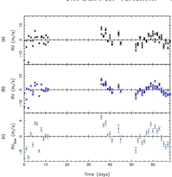
Figure 2. Panel (a): HARPS RV variations in the solar rest-frame, corrected for relativistic Doppler effects (but not yet cor-rected for Vesta’s axial rotation). Panel (b): HARPS RV varia-tions of the Sun as-a-star (after removing the RV contribution of Vesta’s axial rotation). Panel (c): Nightly binned HARPS RV variations of the Sun as-a-star – note the change in scale on the y-axis. The values for each time series are provided in the Sup-plementary Files that are available online.

of applying a conventional barycentric correction, the wave-length scale of the calibrated spectra was adjusted to correct for the Doppler shifts due to the relative motion of the Sun and Vesta, and the relative motion of Vesta and the ob-server (see Section2.3). The FWHM and BIS (as defined in

Queloz et al.(2001)) and log R0HK index were also derived by the pipeline. The median, minimum and maximum signal to noise ratio of the reprocessed HARPS spectra at central wavelength 556.50 nm are 161.3, 56.3 and 257.0, respectively. Overall, HARPS achieved a precision of 75 ± 25 cm s−1 (see Table A1). The reprocessed HARPS cross-correlation functions and derived RV measurements are available in the Supplementary Files that are available online.

We account for the RV modulation induced by Vesta’s rotation in Section 2.4.1, and investigate sources of intra-night RV variations in Section2.4.2. We selected the SDO images in such a way as to compensate for the different view-ing points of Vesta and the SDO spacecraft: Vesta was trail-ing SDO, as shown in Figure1. This is taken into account in Section2.5.

2.2 Solar rest frame

The data reduction pipeline for HARPS assumes that the target observed is a distant point-like star, and returns its RV relative to the solar system barycenter. In order to place the observed RVs of Vesta in the solar rest frame, we perform the following operation:

where RVbary,Earthis the barycentric RV of the Earth, i.e. the component of the observer’s velocity relative to the solar system barycentre, toward the apparent position of Vesta. It can be found in the fits header for each observation. The two components vsv and vve, retrieved from the JPL horizons database2 correspond to:

- vsv: the velocity of Vesta relative to the Sun at the instant that light received at Vesta was emitted by the Sun;

- vve: the velocity of Vesta relative to Earth at the instant that light received by HARPS was emitted at Vesta. This correction accounts for the RV contribution of all bod-ies in the solar system and places the Sun in its rest frame. The values of RVbary,Earth, vsvand vveare given in the Sup-plementary Files that are available online.

2.3 Relativistic Doppler effects

The only relativistic corrections made by JPL horizons are for gravitational bending of the light and relativistic aberration due to the motion of the observer (Giorgini, priv. comm.). We therefore must correct for the relativistic Doppler shifts incurred. The wavelength correction factor to be applied is given byLindegren & Dravins(2003) as:

λe λo = q 1 −v_c22 1 +v cos θo c , (2)

where λe is the wavelength of the light at emission, λo is the wavelength that is seen when it reaches the observer, and θo is the angle between the direction of the emitter at emission and the observed direction of the light at reception. v is the total magnitude of the velocity vector of the observer relative to the emitter, and c is the speed of light.

We apply this correction twice:

- The light is emitted by the Sun and received at Vesta. In this case, v is the magnitude of the velocity of Vesta with respect to the Sun (decreasing from approximately 19.9 to 19.4 km.s−1 over the duration of the HARPS run), and the radial component v cos θo is equal to vsv (defined in Sec-tion 2.2, starting at about 1.66 km.s−1 and reaching 1.72 km.s−1 at opposition near the middle of the run).

- Scattered sunlight is emitted from Vesta and received at La Silla. v is the magnitude of the velocity of Vesta with respect to an observer at La Silla (increasing from 20 to 36 km.s−1 over the run), and v cos θo is vve (starting at 19.8 km.s−1 and reaching 23.3 km.s−1at opposition).

The two wavelength correction factors are then mul-tiplied together in order to compute the total relativistic correction factor to be applied to the pixel wavelengths in the HARPS spectra, from which we derive the correct RVs, shown in Figure2(a) (see also column 2 of Table A1). All velocities are measured at the flux-weighted mid-exposure times of observation (MJDmid UTC).

The reader may also refer to Appendix A ofLanza et al.

2 _{Solar System Dynamics Group, Horizons On-Line}

Ephemeris System, 4800 Oak Grove Drive, Jet Propul-sion Laboratory, Pasadena, CA 91109 USA – Information: http://ssd.jpl.nasa.gov/, Jon.Giorgini@jpl.nasa.gov

(2016) for further details on these Doppler corrections. All quantities used to calculate these effects are listed in the Supplementary Files that are available online.

2.4 Sources of intra-night RV variations 2.4.1 Vesta’s axial rotation

Vesta rotates every 5.34 hours (Stephenson 1951), so any significant inhomogeneities in its shape or surface albedo will induce an RV modulation. Vesta’s shape is close to a spheroid (Thomas et al. 1997), andLanza & Molaro(2015) found that the RV modulation expected from shape inho-mogeneities should not exceed 0.060 m s−1.

Stephenson(1951) presented a photometric study of the asteroid, and suggested that its surface brightness is uneven. He reported brightness variations δm = 0.12 mag. To make a rough estimate of the amplitude of the RV modulation, we can assume that the brightness variations are due to a single dark equatorial spot on the surface of Vesta, blocking a fraction δf of the flux f . δm and δf are related as follows:

δm = 2.5 d(ln f ) log(e) ∼ 1.08

δf

f , (3)

The fractional flux deficit caused by a dark spot can thus be approximated as:

δf

f ∼ δm/1.08 ∼ 0.11. (4)

When the dayside of Vesta is viewed fully illuminated, this spot will give an RV modulation equal to:

∆RVvesta= − δf

f veqcos θ sin θ, (5)

where θ is the angle between the spot on the asteroid and our line of sight, and increases from −π/2 to +π/2 as it traverses the visible daylight hemisphere. Due to foreshortening, the RV contribution is decreased by a factor cos θ. The line-of-sight velocity varies with sin θ. The asteroid’s equatorial velocity veqis given by:

veq= 2π Rvesta

Prot

. (6)

Using a mean radius Rvesta = 262.7 km (Russell et al.

2012) and the rotational period Prot = 5.34 hours, we obtain veq = 85.8 m s−1. The maximum RV amplitude of Vesta’s rotational modulation, expected at θ = π/4 is thus approximately 4.7 m s−1. The RV modulation due to surface brightness inhomogeneity should therefore dominate strongly over shape effects.

We find that this RV contribution is well modelled as a sum of Fourier components modulated by Vesta’s rotation period:

∆RVvesta(t) = C cos(2π − λ(t)) + S sin(2π − λ(t)), (7) where λ(t) is the apparent planetographic longitude of Vesta at the flux-weighted mid-times of the HARPS observations and can be retrieved via the JPL horizons database (the values of λ are listed in Table A1). C and S are scaling parameters, which we determine via a global optimal scal-ing procedure, performed with the solar activity contribu-tions (see Section4.1). Since the phase-folded lightcurve of

Vesta shows a double-humped structure (Stephenson 1951), we also tested adding further Fourier terms modulated by the first harmonic of the asteroid’s rotation. The improve-ment to the fit was negligible, so we preferred the simpler model of Equation7.

Figure2(b) shows the RV observations obtained after subtracting Vesta’s rotational signature, with coefficients C and S of Equation7derived from the global fit of Section4.1. The night-to-night scatter has been reduced, even though much of it remains in the first block of observations; this is discussed in the following Section.

2.4.2 Additional intra-night scatter in first half of HARPS run

The RV variations in the first part of the HARPS run (nights 0 to 11 in Figure2) contain some significant scatter, even af-ter accounting for Vesta’s rotation. This intra-night scataf-ter does not show in the solar FWHM, BIS or log(R0HK) vari-ations. We investigated the cause of this phenomenon and excluded changes in colour of the asteroid or instrumental effects as a potential source of additional noise. Vesta was very bright (7.6 mag), so we deem the phase and proxim-ity of the Moon unlikely to be responsible for the additional scatter observed.

Solar p-mode oscillations dominate the Sun’s power spectrum at a timescale of about 5 minutes. Most of the RV oscillations induced by p-mode acoustic waves are there-fore averaged out within the 15-minute HARPS exposures. Granulation motions result in RV signals of several m s−1, over timescales ranging from about 15 minutes to several hours. Taking multiple exposures each night and averaging them together (as plotted in panel (c) of Figure2) can help to significantly reduce granulation-induced RV variations.

The velocity measurements are sensitive to any dis-placement of the image of Vesta from the centre of the 1-arcsec fibre. Vesta had a finite angular diameter of 0.49 arcsec at the start of the run, and 0.32 arcsec at the end. Light reflected from Vesta is blueshifted by 172 m s−1at the approaching limb and redshifted by 172 m s−1at the reced-ing limb. We simulated the effects of seereced-ing on an ensemble of photons originating from different points on Vesta’s disc, applying random angular deviations with a gaussian see-ing distribution. For a given displacement of Vesta from the centre of the fibre we computed the mean rotational velocity displacement of those photons falling within the fibre. We found an approximately linear dependence of the mean ro-tational velocity on mean offset from the centre of the fibre. Our numerical simulations suggest that a mean displace-ment by 0.1 arcsec of the image from the centre of the fibre in the direction orthogonal to Vesta’s rotation axis, aver-aged over the exposure, gives a velocity error that is closely approximated by the empirical expression:

∆v = 4.0 ( θ 0.4900) / r σseeing 1.000 m s −1 , (8)

where σseeing represents the full width at half-maximum of the gaussian seeing distribution. This is of the same order as the excess RV scatter observed during the first part of the run, when successive observations within a night were widely separated at different airmasses. We conclude that

small airmass-dependent guiding errors provide a plausible explanation. During the latter part of the run, the obser-vations were contiguous and were thus conducted at similar airmass, leading to more consistent guiding and smaller scat-ter. Other factors such as asymmetric image quality, coma of the telescope varying with elevation (and sky rotation on an equatorial telescope), atmospheric dispersion, etc. may also contribute to this effect.

The remaining variations, of order 7-10 m s−1, are mod-ulated by the Sun’s rotation and are caused by the presence of magnetic surface markers, such as sunspots and faculae. These variations are the primary focus of this paper, and we model them using SDO/HMI data in Section3.

2.5 Time lag between Vesta and SDO observations

At the time of the observations, the asteroid Vesta was trail-ing the SDO spacecraft, which orbits the Earth (see Fig-ure1). In order to model the solar hemisphere facing Vesta at time t, we used SDO images recorded at t+∆t, where ∆t is proportional to the difference in the Carrington longitudes of the Earth/SDO and Vesta at the time of the HARPS observation. These longitudes were retrieved from the JPL horizons database. The shortest delay, at the start of the observations was ∼ 2.8 days, while at the end of the ob-servations it reached just over 6.5 days (see Table A1). We cannot account for the evolution of the Sun’s surface fea-tures during this time, and must assume that they remain frozen in this interval. The emergence of sunspots can take place over a few days, but in general large magnetic features (sunspots and networks of faculae) evolve over timescales of weeks rather than days. Visual inspection of animated sequences of SDO images obtained during the campaign re-vealed no major flux emergence events on the visible solar hemisphere.

3 PIXEL STATISTICS FROM SDO/HMI

IMAGES

In the second part of this analysis we aim to determine the RV contribution from granulation, sunspots and facular re-gions. We use high-resolution full-disc continuum intensity, line-of-sight Doppler images and line-of-sight magnetograms from the HMI instrument (Helioseismic and Magnetic Im-ager) onboard SDO3. These were retrieved for the period spanning the HARPS observations of Vesta at times deter-mined by the time lags detailed in Section2.5(the exact date and time stamps of the images are listed in the Supplemen-tary Files that are available online). SDO/HMI images the solar disc in the Fe I 6173˚A line at a cadence of 45 seconds, with a spatial resolution of 1” using a CCD of 4096×4096 square pixels. We first converted the SDO/HMI images from pixel coordinates to heliographic coordinates, i.e. to a coor-dinate system centered on the Sun. This coorcoor-dinate system is fixed with respect to the Sun’s surface and rotates in the sidereal frame once every 25.38 days, which corresponds to

3 _{HMI data products can be downloaded online via the Joint}

Table 1. Solar differential rotation profile parameters from Snod-grass & Ulrich (1990).

Parameter Value (deg day−1₎

α1 14.713

α2 -2.396

α3 -1.787

a Carrington rotation period (Carrington 1859). A surface element on the Sun, whose image falls on pixel ij of the instrument detector, is at position (wij, nij, rij) relative to the centre of the Sun, where w is westward, n is northward and r is in the radial direction (see Thompson (2006) for more details on the coordinate system used). The space-craft is at position (0, 0, rsc). The w, n, r components of the spacecraft’s position relative to each element ij can thus be written as:

δwij= wij− 0 δnij= nij− 0 δrij= rij− rsc

(9)

The spacecraft’s motion and the rotation of the Sun in-troduce velocity perturbations, which we determine in Sec-tions3.1and3.2, respectively. These two contributions are then subtracted from each Doppler image, thus revealing the Sun’s magnetic activity velocity signatures. We compute the RV variations due to the suppression of convective blueshift and the flux blocked by sunspots on the rotating Sun in Sections 3.7.3 and 3.7.2. We show that the Sun’s activity-driven RV variations are well reproduced by a scaled sum of these two contributions in Section4. Finally, we compute the disc-averaged magnetic flux and compare it as an RV proxy against the traditional spectroscopic activity indicators in Section5.

3.1 Spacecraft motion

The w, n, r components of the velocity incurred by the motion of the spacecraft relative to the Sun, vsc, are given in the fits header of each SDO/HMI observation to a precision of 10−6 ms−1. The magnitude of the spacecraft’s velocity away from pixel ij can therefore be expressed as:

vsc,ij= − δwijvsc,wij + δnijvsc,nij + δrijvsc,rij dij , (10) where: dij= q δw2 ij+ δn2ij+ δrij2 (11)

is the distance between pixel ij and the spacecraft. We note that all relative velocities in this paper follow the natural sign convention that velocity is rate of change of distance.

3.2 Solar rotation

The solar rotation as a function of latitude was measured by

Snodgrass & Ulrich(1990) in low resolution full-disc Dopp-lergrams and magnetograms obtained at the Mount Wilson 150 foot tower telescope between 1967 and 1987. By cross-correlating time series of Dopplergrams and magnetograms, they were able to determine the rate of motion of surface

features (primarily supergranulation cells and sunspots) and deduce the rate of rotation of the Sun’s surface as a func-tion of latitude. The solar differential rotafunc-tion profile ω(φ) at each latitude φ is commonly described by a least squares polynomial of the form:

ω(φ) = α1+ α2sin2φ + α3sin4φ. (12) The best fit parameters found by Snodgrass & Ulrich (1990), used in this analysis, are given in Table 1. We apply this rotation profile in the heliographic frame to determine the w, n, r components induced by the solar rotation velocity along the line of sight to a given image pixel, vrot,w, vrot,n and vrot,r. Normalising again by d, we can write:

vrot= −

δw vrot,w+ δn vrot,n+ δr vrot,r

d . (13)

3.3 Flattened continuum intensity

We flatten the continuum intensity images using a fifth order polynomial function Lij with the limb darkening constants given in Astrophysical Quantities (Allen 1973), through the IDL subroutine darklimb correct.pro4. The flattened and non-flattened continuuum intensities are related via the limb-darkening function L as follows:

Iflat,ij= Iij Lij

. (14)

We also define a scaling factor ˆK which will be applied to Lijlater on: ˆ K = P ijIijLijWij P ijL 2 ijWij , (15)

where the weighting factor Wij is set to unity for quiet-Sun pixels, and zero elsewhere.

3.4 Unsigned magnetic field strength

The SDO/HMI instrument measures the line-of-sight mag-netic field strength Bobs. The magnetic field of the Sun stands radially out of the photosphere with a strength Br. Due to foreshortening, the observed field Bobs is less than the true (radial) field by a factor:

µij= cos θij, (16)

where θij is the angle between the outward normal to the feature on the solar surface and the direction of the line-of-sight of the SDO spacecraft.

We can thus recover the full magnetic field strength by dividing by µij:

Br,ij = Bobs,ij/µij. (17)

The noise level in HMI magnetograms is a function of µ (Yeo et al. 2013). It is lowest for pixels in the centre of the CCD, where it is close to 5 G, and increases towards the edges and reaches 8 G at the solar limb. For our analysis we assume that the noise level is constant throughout the image with a conservative value σBobs,ij = 8 G, in agreement with

4 _{Source code available at:}

Figure 3. First three panels: SDO/HMI flattened intensity Iflat, line-of sight velocity v (km s−1) for the non-rotating Sun, and unsigned

radial magnetic flux |Br| (G) of the Sun, observed on 2011, November 10 at 00:01:30 UTC. Last panel: our thresholded image, highlighting

faculae (red/lighter shade pixels) and sunspots (blue/darker shade pixels). For this set of observations (representative of the whole run), faculae account for 9% of the total pixel count, while sunspots account for less than 0.4%. The remaining ∼ 90% of the pixels on the solar disc are magnetically quiet.

the results ofYeo et al.(2013). We therefore set Bobs,ij and Br,ij to 0 for all pixels with a line-of-sight magnetic field measurement (Bobs,ij) below this value.

3.5 Identifying quiet-Sun regions, faculae & sunspots

As is routinely done in solar work, we do not consider pix-els that are very close to the limb (µij < 0.1), as the limb darkening model becomes unreliable on the very edge of the Sun. This affects about 1% of the pixels of the solar disc.

The first three panels of Figure 3 show an SDO/HMI flattened intensitygram, line-of-sight Dopplergram and un-signed radial magnetogram for a set of images taken on 2011, November 10, after removing the contributions from space-craft motion and solar rotation. We identify quiet-Sun re-gions, faculae and sunspots by applying magnetic and in-tensity thresholds.

- Magnetic threshold: The distribution of pixel unsigned observed magnetic field strength as a function of pixel flat-tened intensity is shown in Figure 4. In the top histogram and main panel, we see that the distribution of magnetic

field strength falls off sharply with increasing field strength. The vast majority of pixels are clustered close to the noise level: these pixels are part of the quiet-Sun surface. Note that the fragmented distribution of pixels with magnetic field strength less than a few G arises from the numerical precision in the SDO/HMI images. This is not an issue in our analysis, however, as these pixels are well below the mag-netic noise threshold and we set their field value to zero. We separate active regions from quiet-Sun regions by applying a threshold in unsigned radial magnetic field strength for each pixel.Yeo et al. (2013) investigated the intensity contrast between the active and quiet photosphere using SDO/HMI data, and found an appropriate cutoff at:

|Br,ij| > 3 σBobs,ij/µij, (18)

where σBobs,ij represents the magnetic noise level in each

pixel (see last paragraph of Section 3.4). As in Yeo et al.

(2013), we exclude isolated pixels that are above this thresh-old as they are likely to be false positives. We can thus write:

|Br,thresh,ij| = 24 G /µij. (19)

Sunspots Faculae Quiet Sun Quiet Sun Active regions |Bthresh| Ithresh

Figure 4. Observed pixel line-of-sight (unsigned) magnetic field strength, |Bobs,ij| (G), as a function of flattened intensity Iflat,ij,

for the Sun on 2011, November 10 at 00:01:30 UTC. The top and right histograms show the distributions of |Bobs,ij| and Iflat,ij,

respectively. The dashed lines represent the cutoff criteria selected to define the quiet photosphere, faculae and sunspots.

and the µ-correction for the radial magnetic field strength at the very edge of the solar disc (µij < 0.3) result in a rim of dark pixels being identified as sunspot pixels. In order to avoid this, we set all such pixels as quiet-Sun elements. In any case, sunspots become invisible near the edge of the solar disc because of the Wilson depression (Loughhead & Bray 1958), so our cut should not affect the identification of real sunspot pixels.

- Intensity threshold: The distribution of line-of-sight ve-locity as a function of pixel flattened intensity is shown in Figures 4and5. The main panel allows us to further cate-gorise active-region pixels into faculae and sunspots (umbra and penumbra). We apply the intensity threshold between faculae and spots ofYeo et al.(2013):

Ithresh = 0.89 ˆIquiet, (20)

where ˆIquietis the mean pixel flattened intensity over quiet-Sun regions. It can be calculated by summing the flattened intensity of each pixel:

ˆ Iquiet= P ijIflat,ijWij P ijWij , (21)

where the weighting factor Wij is set to 1 if |Br,ij| < |Br,thresh,ij|, 0 otherwise.

In the main panel of Figure5, quiet-Sun pixels are plotted in black, while active-region pixels are overplotted in yellow. The last panel of Figure 3, which shows the thresholded image according to these Iflat,ijand |Br,ij| criteria, confirms that these thresholding criteria are effective at identifying sunspot and faculae pixels correctly.

Quiet Sun Active regions Sunspots Faculae Quiet Sun Active regions Ithresh

Figure 5. Pixel line-of-sight velocity, vij(in m s−1) , as a

func-tion of flattened intensity Iflat,ij, for the Sun on 2011, November

10 at 00:01:30 UTC. The top and right histograms show the dis-tributions of vijand Iflat,ij, respectively, in bins of 1000. In the

case of active pixels (yellow dots), the line-of-sight velocity is in-variant with pixel brightness. For quiet-Sun pixels (black dots), however, brighter pixels are blueshifted while fainter pixels are redshifted: this effect arises from granular motions.

3.6 Surface velocity flows in sunspot penumbrae and umbrae

The range of velocities in the penumbral pixels (which form the horizontal oval of yellow points just below Ithreshin Fig-ure5) is large owing to the Evershed effect (Evershed 1909). The darker umbral pixels have a narrower velocity distri-bution, allowing the umbral flows that feed the Evershed effect to be resolved into a blueshifted and redshifted veloc-ity component. The much broader range of velocities seen in Figure 5for penumbral vs. umbral pixels confirms that these velocity flows accelerate with distance from the mid-dle of the spot (Evershed 1909). This effect is highlighted in Figure6, which shows a zoom-in on the largest sunspot group in the images of Figure3. The Evershed flows are tan-gential to the surface. They will be most visible for sunspots located away from disc centre, where a larger proportion of them will be directed along our line-of-sight.

The sunspot group illustrated in Figure6is located near the approaching side of the Sun. The flows in its left half are directed away from the observer, while in its right half they are directed towards the observer.

3.7 Decomposing the Sun’s RV into individual feature contributions

The total disc-integrated RV of the Sun is the sum of all contributions from the quiet-Sun, sunspot and faculae/plage regions. The ”quiet” parts of the Sun’s surface are in con-stant motion due to granulation, while sunspots and faculae induce RV variations via two processes (cf. introduction):

Figure 6. Zoom-in on the largest sunspot group on the approach-ing hemisphere of the Sun observed on 2011, November 10 at 00:01:30 UTC. Red pixels represent faculae, while the sunspot pixels are colour-coded according to the direction of their veloc-ity flows, thereby revealing the presence of Evershed flows: dark blue pixels are directed towards the observer (v < 0), while light cyan are directed away from the observer (v > 0).

- Photometric effect: as the Sun rotates, the presence of dark spots or bright faculae on the solar surface breaks the Doppler balance between the approaching (blueshifted) and receding (redshifted) hemispheres. We calculated the contri-bution of dark spots and bright faculae separately and our findings confirm those ofMeunier et al.(2010a), who found that this residual signal is approximately equal to the photo-metric contribution from sunspots. We note, however, that this is merely a coincidence arising from the specific geomet-rical configuration and ratio of sunpots to faculae/plage on the Sun. In other words, this assumption may not be valid for other stars with different spot to faculae configurations and/or filling ratios. We therefore decide to include the effect of faculae in this study (even though it is effectively negli-gible in the case of the Sun). Because the two contributions are correlated (see Figure7), we must account for them in a single term ∆ˆvphot, which we describe in Section3.7.2.

- Convective effect: sunspots and faculae are strongly mag-netised features that inhibit convective motions. Sunspots, which cover a small area of the solar surface and contribute little flux, have a very small contribution. In the case of facu-lae, however, this contribution is large and is expected to be the dominant contribution to the total solar RV variations (Meunier et al. 2010a;Meunier et al. 2010b). We compute this contribution ∆ˆvconvin Section3.7.3.

We can thus write the total disc-integrated RV of the Sun as:

ˆ

v = ˆvquiet+ ∆ˆvphot+ ∆ˆvconv, (22) where ˆvquiet represents the velocity contribution of convec-tive motions in quiet-Sun pixels, which we calculate in Sec-tion3.7.1.

3.7.1 Velocity contribution of convective motions in quiet-Sun regions

We estimate the average RV of the quiet Sun by summing the intensity-weighted velocity of non-magnetised pixels, after

0.4 0.0 0.4

∆ˆ

v

(m

/

s)

∆

ˆ

v

(m

/

s)

Figure 7. Correlation diagram showing the relationship between the rotational Doppler imbalances resulting from sunspots (hor-izontal axis) and faculae (vertical axis), if computed separately. The Spearman correlation coefficient is -0.69. The variations are only partially anti-correlated, reflecting both the tendency of fac-ulae to be spatially associated with sunspot groups and the exis-tence of faculae in bright networks not associated with sunspots. The values of these two basis functions are given in the Supple-mentary Files that are available online.

removing the spacecraft motion and the Sun’s rotation: ˆ vquiet= P ij(vij− δvsc,ij− δvrot,ij) IijWij P ijIijWij . (23)

For this calculation, the weights are defined as in: Wij= 1 if |Br,ij| < |Br,thresh,ij|,

Wij= 0 if |Br,ij| > |Br,thresh,ij|.

(24) This velocity field is thus averaged over the vertical mo-tions of convection granules on the solar surface. Hot and bright granules rise up to the surface, while cooler and darker fluid sinks back towards the Sun’s interior. This process is visible in the main panel of Figure5: quiet-Sun pixels (black dots) are clustered in a tilted ellipse. The area of the upflow-ing granules is larger than that enclosed in the intergranular lanes, and the granules are carrying hotter and thus brighter fluid. This results in a net blueshift, as seen in Figure5.

3.7.2 Rotational Doppler imbalance due to dark sunspots and bright faculae

This velocity perturbation can be obtained by summing the line-of-sight velocity of sunspot pixels corrected for the spacecraft’s motion, and weighted by the flux deficit or ex-cess produced by a dark spot or a bright plage, respectively:

∆ˆvphot= P ij(vij− δvsc,ij) (Iij− ˆK Lij) Wij P ijIij . (25)

The weights Wij are set to 1 for pixels with |Br,ij| > |Br,thresh,ij| (otherwise they are set to 0).

As illustrated in Figure 7, the photometric effects of sunspots and faculae are quite similar in amplitude and roughly anti-correlated, due to their opposite flux signs. However, because they are not strictly anti-correlated they

sum into a net signal that has an amplitude similar to the photometric effect of sunspots (Meunier et al. 2010a). The value of ∆ˆvphot at each time of the HARPS observations is listed in Table A1. From the SDO images we derive an rms amplitude of 0.17 m s−1for this signal, which is smaller than the observational uncertainties of the HARPS veloci-ties. This value is slightly lower than that found byMeunier et al.(2010a) during the peak of the Sun’s activity cycle, of 0.42 m s−1, but remains broadly consistent with their results given the small amplitude of this signal.

3.7.3 Suppression of convective blueshift from active regions

The suppression of granular blueshift induced by magnet-ically active regions (|Br,ij| > |Br,thresh,ij|, predominantly faculae) is:

∆ˆvconv= ˆv − ˆvquiet− ˆvphot. (26) We measure the total disc-averaged velocity of the Sun ˆ

v by summing the velocity contribution of each pixel ij, weighted by their intensity Iij, after subtracting the space-craft motion and solar rotation:

ˆ v = P ij(vij− δvsc,ij− δvrot,ij) Iij P ijIij . (27)

The value of ∆ˆvconvat each time of the HARPS obser-vations is listed in Table A1. The rms amplitude of this basis function (unscaled) is 1.30 m s−1, which is consistent with the value of 1.39 m s−1computed byMeunier et al.(2010a) during the peak of the solar actvity cycle.

4 REPRODUCING THE RV VARIATIONS OF

THE SUN 4.1 Total RV model

We combine our model of Vesta’s rotational RV signal (pre-sented in Section2.4.1) with the two magnetic activity basis functions determined in Sections3.7.3and3.7.2, in order to reproduce the RV variations seen in the HARPS observa-tions. The final model has the form:

∆RVmodel(t) = A ∆ˆvphot(t) + B ∆ˆvconv(t) + ∆RVvesta(t) + RV0. (28) We carry out an optimal scaling procedure in order to determine the scaling factors (A, B, C and S) of each of the contributions, as well as the constant offset RV0 and a constant variance term s2added in quadrature to the ob-servational errors. This variance term will account for any remaining uncorrelated noise arising from granulation mo-tions. The SDO/HMI images were exposed for 45 seconds each, while the HARPS observations were exposed for 15 minutes and binned nightly. We expect these differences to result in a small night-to-night uncorrelated noise contribu-tion. In addition, this variance term will absorb any residual signal of Vesta’s axial rotation, which will naturally not be completely sinusoidal.

For each value of s, the basis functions are orthogo-nalised by subtracting their inverse-variance weighted means prior to performing the scaling. We determine the maximum

(a)

(b)

(c)

(d)

(e)

Figure 8. Panel (a): HARPS RV variations of the Sun as-a-star, ∆RVSun; Panel (b): Scaled basis function for the suppression

of convective blueshift, ∆ˆvconv, derived from SDO/HMI images;

Panel (c): Scaled basis function for the rotational Doppler im-balance due to spots and faculae, ∆ˆvphot; Panel (d): total RV

model, ∆RVmodel (red/lighter shade, with errors including

ad-ditional variance s), overlaid on top of the HARPS RV varia-tions (blue/darker shade points); Panel (e): residuals obtained after subtracting the model from the observations. All RVs are in m s−1_{. Note that the scale of the y-axis is different to that}

used in Figure2. The values of these nightly-binned timeseries are provided in the Supplementary Files available online.

likelihood via a procedure similar to the one described in

Collier Cameron et al. (2006), whereby we maximise the likelihood L of the solution:

ln L = −n 2ln(2π) − 1 2χ 2₋1 2 i=n X i=1 ln(σ2i+ s2) (29) with respect to s, where χ2 _{is the chi-squared value of the n} HARPS data points, with uncertainties σi. This procedure is applied to the unbinned (not nightly-averaged) HARPS dataset, in order to determine the appropriate scaling coef-ficients (C and S) for Vesta’s axial rotation (see Equation7). The total amplitude of the modulation induced by Vesta’s rotation is equal to 2.39 m s−1, which is of the same order as the amplitude we estimated in Section2.4.1.

8

4

0

4

8

∆

RV

(m

/

s)

8

4

0

4

8

∆

R

V

(m

/

s)

Figure 9. HARPS RV variations of the Sun as-a-star vs. our model derived from SDO/HMI images. Observations from the first part of the run are highlighted in a lighter shade.

4.2 Agreement between HARPS observations and SDO-derived model

After all the scaling coefficients were determined, we grouped the observations in each night by computing the inverse variance-weighted average for each night. The final model is shown in Figure8.

We list the best-fit values of the scaling parameters for each of the basis functions in Table 2. We note that the values of A and B, which represent the difference in re-sponse of HARPS and SDO to the Doppler imbalance and the suppression of convective blueshift, differ from unity. The HMI/SDO images are based on measurements of a single spectral line, namely the Fe I 6173˚A line, which may not be representative of the several thousand lines from which the HARPS RVs are derived. The value of ∆ˆvphotis determined by the contrast between the magnetic elements (spots, fac-ulae) and the quiet-Sun photosphere. Most of the lines in the HARPS mask lie blueward of Fe I 6173˚A where the contrast is greater for both types of feature. We therefore expect to have to scale the SDO-derived ∆ˆvphot by a fac-tor of order, but greater than, unity. We measure it to be 2.45±2.02; the amplitude of ∆ˆvphotis so small that A cannot be distinguished from unity when the additional variance s is taken into account. The strength of the convection inhibi-tion changes with line depth (cf. Gray(2009) andMeunier et al. (2010b)). We find that the HARPS response to sup-pression of granular blueshift is 1.85 ± 0.27 times greater than we predict from SDO.

We show a plot of the observed HARPS RVs (∆RVSun) vs. our SDO-modelled RVs (∆RVmodel) in Figure 9, in a similar fashion to Figure 9 of Meunier et al. (2010b). We see good agreement between the data and the model. The Spearman correlation coefficient is 0.64 for the full dataset and 0.87 when considering only the second part of the run. This is close to, although not as good as the correlation coef-ficient of 0.94 found byMeunier et al.(2010b) between sim-ulated velocities ofMeunier et al.(2010a) and MDI/SOHO Dopplergrams.

Panel (e) of Figure8shows the residuals remaining af-ter subtracting the total model ∆RVmodelfrom the HARPS

Table 2. Best-fit parameters and rms amplitudes resulting from the optimal scaling procedure.

Parameter Value Basis function rms amplitude (unscaled) A 2.45 ± 2.02 ∆ˆvphot 0.17 m s−1 B 1.85 ± 0.27 ∆ˆvconv 1.30 m s−1 C 2.19 ± 0.42 cos(2π − λ) 0.74 m s−1 S 0.55 ± 0.47 sin(2π − λ) 0.66 m s−1 RV0 99.80 ± 0.28 m s−1 s 2.70 m s−1

observations of the Sun as-a-star ∆RVSun. We see that the residuals are within the level of the error bars, when con-sidering an extra variance term s of 2.7 m s−1. Maximum-likelihood analysis of the additional uncorrelated noise dur-ing the first part of the run (nights 0-11) yields an additional variance with rms amplitude 4.0 m s−1, while the second part (nights 36-68) has an additional noise rms of 1.5 m s−1. As discussed in Section2.4.2, we attribute the excess scat-ter in the first block of nights to airmass-dependent guiding errors, which would have been more important in the first part of the run, where the observations within each night were taken at very different airmasses. The additional noise rms of 1.5 m s−1 in the second part of the run is consistent with the rms due to solar granulation and super-granulation, ranging between 0.28 and 1.12 m s−1, as recently found by

Meunier et al.(2015).

4.3 Relative importance of suppression of convective blueshift and rotational velocity imbalance

We see that the activity-induced RV variations of the Sun are well reproduced by a scaled sum of the two basis functions, ˆ

vconvand ˆvphot(shown in Figure8panels (b) and (c), respec-tively). As previously predicted byMeunier et al. (2010a), we find that the suppression of convective blueshift plays a dominant role (rms of 2.40 m s−1). This was also found to be the case for CoRoT-7, a main sequence G9 star with a rotation period comparable to that of the Sun (Haywood et al. 2014). The relatively low amplitude of the modula-tion induced by sunspot flux-blocking (rms of 0.17 m s−1) is expected in slowly-rotating stars with a low v sin i (Desort et al. 2007).

4.4 Zero point of HARPS

The wavelength adjustments that were applied to the HARPS RVs were based on precise prior dynamical knowl-edge of the rate of change of distance between the Earth and Vesta, and between Vesta and the Sun. The offset RV0 = 99.80 ± 0.28 m s−1 thus represents the zero point of the HARPS instrument, including the mean granulation blueshift for the Sun. A previous study of integrated sunlight reflected by the Moon, byMolaro et al.(2013), determined a value of 102.2 ± 0.86 m s−1, which is significantly larger than our value. They did not account for the effect of sunspots

8 4 0 4 8 ∆

R

V

/

B

G

v

/

f

FWHM

/

BIS

/

R

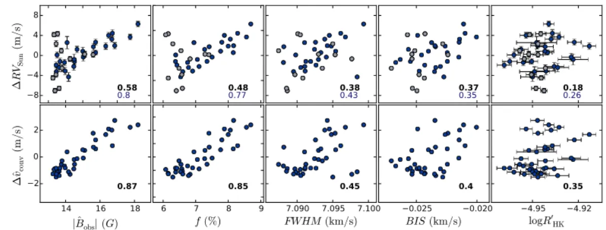
Figure 10. Correlation plots of the nightly-averaged HARPS RV variations of the Sun as-a-star ∆RVSunand suppression of convective

blueshift ∆ˆvconvagainst (from left to right): the disc-averaged observed magnetic flux | ˆBobs| (G), filling factor f (%), FWHM (km s−1),

BIS (m s−1) and log(R0_HK). Observations from the first part of the run are highlighted in a lighter shade. Spearman correlation coefficients are displayed in the bottom-right corner of each panel: for the full observing run (in bold and black), and for the second part of the run only (in blue).

and faculae, however, so their result could be affected by activity-induced solar variations at that time.

5 TOWARDS BETTER PROXIES FOR RV

OBSERVATIONS

5.1 Spatial distributions of sunpots and faculae

Aigrain et al.(2012) have shown that it is possible to predict the rotational Doppler imbalance due to photospheric sur-face brightness inhomogeneities from a simultaneous high-precision optical lightcurve. If one further assumes that facu-lae/plage regions are co-spatial with spot groups, then they can also predict the form of the RV variation caused by suppression of granular blueshift. A recent analysis of the active host star CoRoT-7 by Haywood et al.(2014) mod-elled activity-induced RV variations via the FF’ method of

Aigrain et al.(2012). The predicted Doppler imbalance was much smaller than the observed activity-driven RV varia-tions. The associated suppression of convective blueshift was of larger amplitude than, and partially correlated with, the observed RVs. The residuals, however, had a similar am-plitude and shared the covariance properties of the star’s (simultaneous) lightcurve.

The present study provides a natural explanation of this mismatch: on the Sun, the faculae are not perfectly co-spatial with sunspot groups. Indeed, Figure7shows us that the location of sunspot groups give an incomplete prediction of the facular coverage. Since the suppression of granular blueshift is the dominant process at play in slowly-rotating stars such as CoRoT-7 and the Sun, it is therefore important to develop proxies that are directly sensitive to the distribu-tion of faculae on the stellar surface.

5.2 Correlations between RV and traditional activity indicators

Figure10presents the correlations between ∆RVSun, ∆ˆvconv and the following activity indicators: the full-disc magnetic

flux | ˆBobs| and filling factor f computed from the SDO/HMI images, and the observed FWHM, BIS, and log(R0HK) de-rived from the HARPS DRS reduction pipeline. We com-puted the Spearman correlation coefficent to get a measure of the degree of monotone correlation between each variable (the correlation between two variables is not necessarily lin-ear, for example between RV and BIS). The coefficients are displayed in each panel of Figure10, both including and ex-cluding the observations made in the first part of the run, which show a lot of intra-night scatter.

We do not show similar correlation plots for ∆ˆvphot be-cause we do not find any significant correlations with any of the activity indicators; this is expected since ∆ˆvphot is such that it crosses zero when the surface covered by spots and/or faculae is at a maximum, i.e. when they are in the middle of the stellar disc (∆ˆvphotis of course still related to | ˆBobs|, the FWHM, BIS, and log(R0HK), but the Spearman coefficient is close to zero).

We note that the relatively weak correlation between the observed RVs and the BIS is not completely unexpected in the case of the Sun, which has a v sin i of about 2 km s−1. The line profile distortions induced by solar activity, includ-ing those measured by the BIS, will therefore be smaller than the resolution of HARPS that is close to 2.5 km s−1. In other words, the resolution of HARPS is not adequate to fully resolve the BIS variations in a star rotating as slowly as the Sun, which could reduce the correlation coefficients computed with the BIS.

We find a relatively weak correlation between the ob-served RVs and the chromospheric flux index log(R0HK), with a Spearman correlation coefficient of 0.26 for the second half of the run (0.18 for the full run).

Although naively one might expect log(R0HK) to be a good predictor of plage filling factor, and hence of the con-vective RV component, there are several physical factors that might reasonably be expected to degrade the corre-lation over short time scales (our dataset spans 2-3 solar ro-tations). Foreshortening and limb darkening affect the Ca II HK emission cores and the brightness-weighted line-of-sight granular velocities in different ways. Near the limb, the Ca

(a) (b) (c) (d) (e) (f)

Figure 11. Panel (a): HARPS RV variations of the Sun as-a-star; panels (b) and (c): time series of the disc-averaged line-of-sight magnetic flux | ˆBobs| and filling factor f , respectively, determined

from the SDO/HMI magnetograms; panels (d), (e) and (f ): time series of the FWHM, BIS and log(R0_HK), respectively, determined from the HARPS DRS reduction pipeline. The values of these nightly-binned timeseries are provided in the Supplementary Files available online.

II emission in plages originates in higher, hotter regions of the chromosphere and remains bright. The limb darkening of facular pixels is less than that of quiet-sun pixels, but near the limb the line-of-sight component of the radial motion of bright granule cores is reduced by foreshortening. The disc-averaged line-of-sight magnetic field strength is attenuated by both foreshortening and limb darkening in approximately the same way as the radial motion of the granular flow. This may explain why, even though the RVs and log(R0HK) values were measured simultaneously from the same spectra, the correlation between the variations in log(R0HK) and suppres-sion of granular blueshift appears weak. In their study of

long-term solar RV variations spanning over 8 years,Lanza et al.(2016) find a stronger correlation between log(R0HK) and RV variations, with a Spearman coefficient of 0.357. This positive correlation is in agreement with previous studies of quiet late-type stars (Gomes da Silva et al. 2012;Lovis et al. 2011), and shows that the log(R0HK) may be a more useful proxy for long-term RV variations induced the stellar mag-netic cycle.

We note that in Figure10, the variations in log(R0HK) look similar to the variations in RV, except that they are shifted by a few days (this is especially noticeable towards the end of the run). The reality and origin of this shift will be the subject of future studies, thanks to the wealth of Sun as-a-star RV observations that are currently being gathered by the solar telescope at HARPS-N.

5.3 Disc-averaged observed magnetic flux | ˆBobs| We compute the full-disc line-of-sight magnetic flux of the Sun, by summing the intensity-weighted line-of-sight un-signed magnetic flux in each pixel:

| ˆBobs| = P ij|Bobs,ij| Iij P ijIij . (30)

The values at the time of each HARPS observation are listed in Table A1. The variations in | ˆBobs| are shown in panel (b) of Figure11, together with the nightly-averaged HARPS RV variations of the Sun as-a-star, in panel (a). We see that the variations in the disc-averaged magnetic flux are in phase with the RV variations, despite the scatter in RV in the first part of the run (discussed in Section2.4.2). If we only consider the observations in the second part of the run, the Spearman correlation coefficient between ∆RVSun and | ˆBobs| is 0.80 (see Figure 10). The correlation is stronger between ˆvconv and | ˆBobs|, with a correlation coefficient of 0.87. This is expected since magnetised areas are known to suppress convective blueshift (see Meunier et al. (2010a);

Meunier et al.(2010b)).

We note that these observations were taken close to the solar cycle maximum, during which the solar photosphere was mostly dominated by a few large sunspot groups (sur-rounded by facular networks).Meunier et al.(2010b) found that the convective shift attenuation is greater in larger structures, since they contain a stronger magnetic field. The relationship between convective shift attenuation and mag-netic field, however, is not linear. We thus expect larger RV variations for a few large active regions than when the Sun is in a phase of lower magnetic activity, when the photo-sphere might be dominated by several smaller structures, even though they would still give the same total flux. In fact,Lanza et al.(2016) find a much weaker correlation be-tween the mean total magnetic flux measured by the SOLIS VSM instrument and RV (Spearman correlation coefficient of 0.131) over their 8-year dataset, which spans both active and less active phases of the solar cycle.

When compared against correlations with the tradi-tional spectroscopic activity indicators (the FWHM, BIS and log(R0HK)), we see that the disc-averaged magnetic flux | ˆBobs| is a much more effective predictor of activity-induced RV variations, over the timescale of a few rotation periods. The averaged magnetic flux may therefore be a useful proxy for activity-driven RV variations as it should map onto areas

of strong magnetic fields, which suppress the Sun’s convec-tive blueshift. The line-of-sight magnetic flux density and filling factor on the visible hemisphere of a star can be mea-sured from the Zeeman broadening of magnetically-sensitive lines (Robinson 1980; Reiners et al. 2013). Their product gives the disc-averaged flux density that we are deriving from the solar images. We note that such measurements are still very difficult to make for other stars than the Sun, be-cause the Zeeman splitting of magnetically sensitive lines is so small that the technique can only be applied to bright, slowly rotating stars. Fortunately, such stars are also the best targets for planet searches.

5.4 Magnetic filling factor f

In addition to the disc-averaged observed magnetic flux, we also computed the filling factor of magnetic regions on the solar disc. It is weighted by the foreshortening at the location of each pixel, and counted as a fraction of the total pixel count: f = 1 Npix X ij Wij, (31)

where Npix is the total number of pixels in the solar disc and the weight Wijis set to 1 in magnetically active regions, and 0 in the quiet Sun. The variations of the filling factor are shown in panel (c) of Figure11. As expected, they follow the disc-averaged magnetic flux closely. The correlation with the predicted ∆RVconvand the observed ∆RVSunis nonetheless weaker than that found for the brightness-weighted line-of-sight magnetic field | ˆBobs|, since no correction is made for limb darkening.

6 CONCLUSION

In the present analysis, we decomposed activity-induced radial-velocity (RV) variations into identifiable contributions from sunspots, faculae and granulation, based on Sun as-a-star RV variations deduced from HARPS spectra of the bright asteroid Vesta and high spatial resolution images in the Fe I 6173 ˚A line taken with the Helioseismic and Mag-netic Imager (HMI) instrument aboard the Solar Dynamics Observatory (SDO). We find that the RV variations induced by solar activity are mainly caused by the suppression of convective blueshift from magnetically active regions, while the flux deficit incurred by the presence of sunspots on the rotating solar disc only plays a minor role. We further com-pute the disc-averaged line-of-sight magnetic flux and show that although we cannot yet measure it with precision on other stars at present, it is a very good proxy for activity-driven RV variations, much more so than the full width at half-maximum and bisector span of the cross-correlation pro-file, and the Ca II H&K activity index. These findings are in agreement with the previous works ofMeunier et al.(2010a) andMeunier et al.(2010b).

In addition to the existing 2011 HARPS observations of sunlight scattered off Vesta, there will soon be a wealth of direct solar RV measurements taken with HARPS-N, which will be regularly fed sunlight through a small 2-inch tele-scope developed specifically for this purpose. A prototype for this is currently being commissioned at HARPS-N (see

Dumusque et al. (2015), Glenday et al. (in prep.)). Gain-ing a deeper understandGain-ing of the physics at the heart of activity-driven RV variability will ultimately enable us to better model and remove this contribution from RV obser-vations, thus revealing the planetary signals.

ACKNOWLEDGMENTS

We wish to thank the referee for their thoughtful comments, which have greatly helped improve the analysis presented in this paper. RDH gratefully acknowledges STFC studentship grant number ST/J500744/1, and a grant from the John Templeton Foundation. The opinions expressed in this pub-lication are those of the authors and do not necessarily re-flect the views of the John Templeton Foundation. ACC and RF acknowledge support from STFC consolidated grants numbers ST/J001651/1 and ST/M001296/1. JL acknowl-edges support from NASA Origins of the Solar System grant No. NNX13AH79G and from STFC grant ST/M001296/1. The Solar Dynamics Observatory was launched by NASA on 2011, February 11, as part of the Living With A Star pro-gram. This research has made use of NASA’s Astrophysics Data System Bibliographic Services.

REFERENCES

Aigrain S., Pont F., Zucker S., 2012, Monthly Notices of the Royal Astronomical Society, 419, 3147

Allen C., 1973, Allen: Astrophysical Quantities (3rd edn.) The Athlone Press - Google Scholar. University of London Baranne A., et al., 1996, Astronomy and Astrophysics

Supple-ment Series, 119, 373

Boisse I., et al., 2009, Astronomy and Astrophysics, 495, 959 Boisse I., Bouchy F., H´ebrard G., Bonfils X., Santos N., Vauclair

S., 2011, Astronomy and Astrophysics, 528, A4

Bonfils X., et al., 2007, Astronomy and Astrophysics, 474, 293 Brandt P. N., Solanki S. K., 1990, A&A,231, 221

Carrington R. C., 1859, Monthly Notices of the Royal Astronom-ical Society, 19, 81

Chapman G. A., Cookson A. M., Dobias J. J., Walton S. R., 2001, ApJ,555, 462

Collier Cameron A., et al., 2006, Monthly Notices of the Royal Astronomical Society, 373, 799

Deming D., Plymate C., 1994, Astrophysical Journal, 426, 382 Deming D., Espenak F., Jennings D. E., Brault J. W., Wagner

J., 1987, Astrophysical Journal, 316, 771

Desort M., Lagrange A. M., Galland F., Udry S., Mayor M., 2007, Astronomy and Astrophysics, 473, 983

D´ıaz R. F., et al., 2015, preprint, (arXiv:1510.06446) Dumusque X., et al., 2011,A&A,535, A55

Dumusque X., et al., 2015,ApJ,814, L21 Evershed J., 1909, MNRAS,69, 454 Glenday A., Phillips D. F., et al. in prep.

Gomes da Silva J., Santos N. C., Bonfils X., Delfosse X., Forveille T., Udry S., Dumusque X., Lovis C., 2012,A&A,541, A9 Gray D. F., 2009,ApJ,697, 1032

Gregory P. C., 2011,MNRAS,415, 2523

Hall J. C., 2008, Living Reviews in Solar Physics, 5, 2

Haywood R. D., et al., 2014, Monthly Notices of the Royal Astro-nomical Society, Volume 443, Issue 3, p.2517-2531, 443, 2517 Hu´elamo N., et al., 2008, Astronomy and Astrophysics, 489, L9 Isaacson H., Fischer D., 2010,ApJ,725, 875

Jim´enez A., Pall´e P. L., R´egulo C., Roca Cortes T., Isaak G. R., 1986, COSPAR and IAU, 6, 89

Lagrange A. M., Desort M., Meunier N., 2010, Astronomy and Astrophysics, 512, A38

Lanza A. F., Molaro P., 2015,Experimental Astronomy,39, 461 Lanza A. F., Molaro P., Monaco L., Haywood R. D., 2016,

preprint, (arXiv:1601.05646) Lean J., 1997,ARA&A,35, 33

Lindegren L., Dravins D., 2003, Astronomy and Astrophysics, 401, 1185

Loughhead R. E., Bray R. J., 1958,Australian Journal of Physics, 11, 177

Lovis C., Pepe F., 2007, Astronomy and Astrophysics, 468, 1115 Lovis C., Dumusque X., Santos N. C., Udry S., Mayor M., 2011, AAS/Division for Extreme Solar Systems Abstracts, 2, 0202 McMillan R. S., Moore T. L., Perry M. L., Smith P. H., 1993,

ApJ,403, 801

Meunier N., Desort M., Lagrange A. M., 2010a, Astronomy and Astrophysics, 512, A39

Meunier N., Lagrange A.-M., Desort M., 2010b,A&A,519, A66 Meunier N., Lagrange A.-M., Borgniet S., Rieutord M., 2015,

A&A,583, A118

Molaro P., Centuri´on M., 2010, Astronomy and Astrophysics, 525, A74

Molaro P., Monaco L., Barbieri M., Zaggia S., 2013, Monthly Notices of the Royal Astronomical Society: Letters, 429, L79 Murdin P., 2002, Encyclopedia of Astronomy and Astrophysics,

-1

Pesnell W. D., Thompson B. J., Chamberlin P. C., 2012, Solar Physics, 275, 3

Queloz D., et al., 2001, Astronomy and Astrophysics, 379, 279 Reiners A., Shulyak D., Anglada-Escud´e G., Jeffers S. V., Morin

J., Zechmeister M., Kochukhov O., Piskunov N., 2013, As-tronomy and Astrophysics, 552, 103

Robertson P., Mahadevan S., Endl M., Roy A., 2014, Science, 345, 440

Robinson Jr. R. D., 1980,ApJ,239, 961 Russell C. T., et al., 2012, Science, 336, 684

Santos N. C., Gomes da Silva J., Lovis C., Melo C., 2010,A&A, 511, A54

Santos N. C., et al., 2014, Astronomy and Astrophysics, 566, 35 Schou J., et al., 2012, Solar Physics, 275, 229

Schrijver C. J., 2002, Astronomische Nachrichten, 323, 157 Snodgrass H. B., Ulrich R. K., 1990, Astrophysical Journal, 351,

309

Stephenson C. B., 1951, Astrophysical Journal, 114, 500 Thomas P. C., Binzel R. P., Gaffey M. J., Zellner B. H., Storrs

A. D., Wells E., 1997, Icarus, 128, 88

Thompson W. T., 2006, Astronomy and Astrophysics, 449, 791 Yeo K. L., Solanki S. K., Krivova N. A., 2013,A&A,550, A95 This paper has been typeset from a TEX/LA_{TEX file prepared by}