HAL Id: hal-00317502
https://hal.archives-ouvertes.fr/hal-00317502
Submitted on 31 Jan 2005
HAL is a multi-disciplinary open access
archive for the deposit and dissemination of
sci-entific research documents, whether they are
pub-lished or not. The documents may come from
teaching and research institutions in France or
abroad, or from public or private research centers.
L’archive ouverte pluridisciplinaire HAL, est
destinée au dépôt et à la diffusion de documents
scientifiques de niveau recherche, publiés ou non,
émanant des établissements d’enseignement et de
recherche français ou étrangers, des laboratoires
publics ou privés.
ion-neutral dynamics using co-located tristatic FPIs and
EISCAT radar in Northern Scandinavia
A. L. Aruliah, E. M. Griffin, A. D. Aylward, E. A. K. Ford, M. J. Kosch, C. J.
Davis, V. S. C. Howells, S. E. Pryse, H. R. Middleton, J. Jussila
To cite this version:
A. L. Aruliah, E. M. Griffin, A. D. Aylward, E. A. K. Ford, M. J. Kosch, et al.. First direct evidence
of meso-scale variability on ion-neutral dynamics using co-located tristatic FPIs and EISCAT radar in
Northern Scandinavia. Annales Geophysicae, European Geosciences Union, 2005, 23 (1), pp.147-162.
�hal-00317502�
SRef-ID: 1432-0576/ag/2005-23-147 © European Geosciences Union 2005
Annales
Geophysicae
First direct evidence of meso-scale variability on ion-neutral
dynamics using co-located tristatic FPIs and EISCAT radar in
Northern Scandinavia
A. L. Aruliah1, E. M. Griffin1, A. D. Aylward1, E. A. K. Ford1, M. J. Kosch2, C. J. Davis3,1, V. S. C. Howells3, S. E. Pryse4, H. R. Middleton4, and J. Jussila5
1University College London, 67-73, Riding House Street, London W1W 7EJ, UK
2Department of Communications Systems, Lancaster University, Lancaster, LA1 4YR, UK
3Space Science and Technology Department, CCLRC Rutherford Appleton Laboratory, Chilton, Didcot, Oxfordshire, OX11
0QX, UK
4Institute of Mathematical and Physical Sciences, University of Wales Aberystwyth, Ceredigion SY23 3BZ, Wales, UK 5Department of Physical Sciences, P.O. Box 3000, FIN-90014, University of Oulu, Finland
Received: 1 March 2004 – Revised: 8 November 2004 – Accepted: 9 November 2004 – Published: 31 January 2005 Part of Special Issue “Eleventh International EISCAT Workshop”
Abstract. This paper presents the first direct empirical
ev-idence that mesoscale variations in ion velocities must be taken into consideration when calculating Joule heating and relating it to changes in ion temperatures and momentum transfer to the neutral gas. The data come from the first tristatic Fabry-Perot Interferometer (FPI) measurements of the neutral atmosphere co-located with tristatic measure-ments of the ionosphere made by the European Incoher-ent Scatter (EISCAT) radar which were carried out during the nights of 27–28 February 2003 and 28 February until 1 March 2003. Tristatic measurements mean that there are no assumptions of uniform wind fields and ion drifts, nor zero vertical winds. The independent, tristatic, thermospheric measurements presented here should provide unambiguous vector wind information, and hence reduce the need to sup-plement observations with information obtained from mod-els of the neutral atmosphere, or with estimates of neutral parameters derived from ionospheric measurements. These new data can also test the assumptions used in models and in ion-neutral interactions. The FPIs are located close to the 3 radars of the EISCAT configuration in northern Scandi-navia, which is a region well covered by a network of com-plementary instruments. These provide a larger scale context within which to interpret our observations of mesoscale vari-ations on the scales of tens of kilometres spatially and min-utes temporally. Initial studies indicate that the thermosphere is more dynamic and responsive to ionospheric forcing than expected. Calculations using the tristatic volume measure-ments show that the magnitude of the neutral wind dynamo
Correspondence to: A. L. Aruliah
contribution was on average 29% of Joule heating during the first night of observation. At times it either enhanced or re-duced the effective electric field by up to several tens of per-cent. The tristatic experiment also presents the first valida-tion of absolute temperature measurements from a common volume observed by independently calibrated FPIs. Com-parison of EISCAT ion temperatures at an altitude of 240 km with FPI neutral temperatures show that Tiwas around 200 K
below Tnfor nearly 3 h on the first night during a period of
strong geomagnetic activity. This is inconsistent with en-ergy transfer. Comparison with FPI temperatures from sur-rounding regions indicate that it could not be accounted for by height variations. Indeed, these first results seem to in-dicate that the 630-nm emission did not stray too far from 240 km. There were also apparent drops in Te at the same
time as the anomalous Ti values which are energetically
implausible. Incorrect assumptions of composition or non-Maxwellian spectra are likely to be the problem.
Key words. Ionosphere (Auroral ionosphere; Electric fields
and currents; Ionosphere-atmosphere interactions)
1 Introduction
This is a unique experiment where a common volume is ob-served by the EISCAT radar and 3 FPIs to permit indepen-dent and tristatic measurements of the ionosphere and ther-mosphere, respectively. The first true common volume ob-servations were made by the Dynamics Explorer 2 space-craft, which carried an FPI and spectrometer instrument to measure the neutral component, together with an ion drift
Fig. 1. Location of the 3 FPIs at Skibotn, KEOPS and Sodankyl¨a
and the EISCAT radar at Tromsø. The circles show the field-of-view of the FPIs for elevation angles of 51.5◦for Skibotn and 45◦ for KEOPS and Sodankyl¨a. The dots indicate the positions of the volumes viewed by each FPI. Positions A and B are the tristatic and bistatic volumes, respectively. The locations of the IMAGE magnetometers are also given.
meter and retarding potential analyzer instrument for the ionospheric component (Killeen et al., 1984). The majority of previous ground-based experiments mainly investigated large-scale behaviour over a region of hundreds of kilome-tres using a single FPI with a radar (e.g. Cierpka et al., 2000; Aruliah and Griffin, 2001; Sakonoi et al., 2002). There are only a small number of published meso-scale investigations using two FPIs in close proximity (i.e. Greet et al., 1999; Ishii et al., 2001).
At present the mainland EISCAT radar is the only radar in the world that makes true tristatic observations of the ionosphere. This is achieved using a transmitter/receiver at Tromsø and receivers at Kiruna and Sodankyl¨a. Other radars derive plasma velocities using a single transmitter/receiver and rely on beam-swinging techniques with the assump-tion that the plasma velocity field is unchanged between two directions of observation. The limitations of the beam-swinging technique are presented by Etemadi et al. (1989) and are particularly pertinent since the small-scale variability of the ionosphere has now become a prime concern. Merg-ing and reconnection of the solar wind with the geomagnetic field is no longer seen to be a steady-state phenomenon, but a series of irregular pulsed events resulting in highly variable plasma velocities (Lockwood et al., 1995). A major short-coming of the models is that there are large disparities in the values of neutral winds and temperatures between model calculations and observations. The general circulation mod-els (GCMs) use large-scale averaged electric fields and par-ticle precipitation models which result in too much momen-tum transferred to the neutral gas, and too little Joule heat-ing at high-latitudes. Put simply, the effect of applyheat-ing a
constant drag term (albeit a smaller force than the instanta-neous force) compared with a semi-random force vector that swings rapidly about a near zero average value, results in a building up of velocities which are not observed in the real atmosphere. Similarly, the heating effect of a smoothly aver-aged plasma flow is significantly smaller than that of a ran-domly varying flow. The lack of consideration of small-scale variability is a serious limitation of the models and conse-quently an important new area of investigation.
Papers are beginning to appear that show that the high-latitude thermosphere also has small-scale variability (e.g. Conde et al., 2001; Aruliah and Griffin, 2001; Aruliah et al., 2004) and in particular with connection to gravity waves (In-nis and Conde, 2002). This is important since the neutral winds and temperatures appear in several fundamental equa-tions for ion-neutral dynamics and energetics. Unfortunately, the main sources of observation of the neutral component of the upper atmosphere are passive, such as optical emissions which are all spatially and temporarily localised, and satel-lite drag, which has its own spatial and temporal sacrifices in order to obtain global coverage. Consequently, the lack of available thermospheric data has meant that assumptions are frequently used instead of observations. As a result the as-sumptions of a slowly varying inertial medium are ingrained and the need for contemporaneous data collection is often overlooked. However, the substitution of model data brings problems, since models are an excellent tool for understand-ing general mechanisms, but are inadequate as a replacement since they will propagate the limitations of their assumptions. Even empirical models can only substitute for generic clima-tology studies.
2 The tristatic experiment
The first tristatic campaign was held during the period 16:30– 04:30 UT on the nights of 27–28 February 2003 and 28 February until 1 March 2003. Figure 1 shows the location of the instruments in the auroral zone in Northern Scandi-navia. The FPIs observe the red line emission at 630 nm of atomic oxygen which is the second most dominant nighttime auroral and airglow emission after the green line emission at 557.7 nm, in the visible region. The height of the red line emission peak intensity is around 240 km (e.g. Solomon et al., 1988), thus the Doppler shifts and Doppler broadening of the emission allows for the calculation of the wind speeds and temperatures of the upper thermosphere.
The three FPIs are at the Sodankyl¨a Geophysical Ob-servatory in Finland (67.4◦N, 26.6◦E), Skibotn in Nor-way (69.3◦N, 20.4◦E) and the Kiruna Esrange Optical Site (KEOPS) in Sweden (67.8◦N, 20.4◦E). Each FPI observes a 1◦ field-of-view at an elevation angle of 45◦ for the So-dankyl¨a and KEOPS FPIs, and 51.5◦ for the Skibotn FPI. A scanning mirror turns to allow for observation to the north, east, south, west and zenith, thus providing a large-scale con-text by creating a grid of FPI observations of winds, temper-atures and intensities. The circles define the viewing area of
each FPI, assuming an emission height of 240 km. Two fur-ther positions are observed: position A is the tristatic com-mon volume, where the fields-of-view of all three FPIs over-lap, and position B is a bistatic common volume seen by the KEOPS and Sodankyla FPIs. As can be seen from Fig. 1, there are also other points where more than one FPI can view volumes that are in close proximity, such as KEOPS zenith with Sodankyl¨a west and Skibotn south viewing volumes.
The EISCAT radar was in CP1-like mode. The CP1 mode is a fixed transmitter beam in the field-aligned direction, however, in this experiment the beam and the two receivers are not field-aligned, but are aimed at the common volume A (69.4◦N, 25.0◦E), to make tristatic measurements. Further details of the operation of the FPIs may be found in Aruliah and Griffin (2001), and of the EISCAT radar in Rishbeth and Williams (1985).
The FPIs are not cross calibrated for intensity and so each has been scaled to match the KEOPS FPI intensity in the fig-ures shown in this paper. Each FPI is of a different age and there are different detector sensitivities. Detector technology has progressed rapidly over the 10 years since the Skibotn FPI was built. The Skibotn FPI (intensified EEV detector) has an integration time of 60 s, while the Sodankyl¨a (EEV detector) and KEOPS (Andor detector) FPI have 40 and 20 s, respectively. Consequently the time resolution to complete a cycle of observations is 3.5 min and 8.5 min for the KEOPS and Sodankyl¨a FPIs, respectively. The Skibotn FPI has a cycle time of 13.9 min, however, the tristatic A position is viewed twice in each cycle to improve the time resolution. The reason for the low time resolution is that the Skibotn FPI has a longer dead time owing to its more complex me-chanical system which includes additional mirror elevation control. This accounts for why the Skibotn FPI misses the variability and dramatic peaks in intensity seen by the other 2 FPIs and also misses out on data when the signal-to-noise ratio is too poor. The intensities of the Sodankyl¨a and Ski-botn FPIs have been scaled to the KEOPS intensities by mul-tiplying by factors of 11.4 and 1.49, respectively. Having scaled the data, the difference in intensities can be attributed to several possible contributions:
1. Longer FPI integration times and lower time resolutions smooth out the sharp peaks and troughs seen by the highest resolution FPI at KEOPS.
2. If the emission peak height is greater or smaller than 240 km, the line-of-sight observing volume of each FPI will over- or undershoot A and so there is no longer a common volume.
3. The height integrated intensities from the 3 FPI view-points are different,owing to the variations in the emis-sion profiles over the fields-of-view.
4. Cloud scatter.
Comparison of the intensities and temperatures of all the look directions allow for an investigation of variability on scales of tens of kilometres to a few hundred kilometres.
The spatial scale size of the thermosphere will determine whether (b) and (c) make much difference to the height-integrated intensity. Current models such as the GLOW model (Solomon et al., 1988) have too coarse a spatial resolu-tion, owing to their dependence on parameters derived from global models, such as the International Reference Iono-sphere (IRI) (Bilitza, 1997) and MSIS (Picone et al., 2002), to show any significant variation for less than 5◦ latitude. This is a severe limitation of global models, since the upper atmosphere at high-latitudes is highly spatially variable, and the region covered by the 3 FPIs is around 6◦latitude by 18◦ longitude. As an example, this region would be represented by only 3 points in the CTIP model, which currently has a spatial resolution of 2◦latitude by 18◦longitude (e.g. Mill-ward et al., 1996). However, the model’s spatial limitation can be helped by using a 1-min time step and equating Local Time variations with longitude variations.
The geometry of the location of the FPIs is not ideal. The best configuration would be for the 3 FPIs to be at the cor-ners of an equilateral pyramid with the common volume at the apex. The FPI geometry is determined by the location of the facilities of the three geophysical institutes housing the EISCAT radars. The Skibotn FPI points almost to the east to view the tristatic A position. As a result, it measures an extremely small meridional component. Thus, the tristatic zonal component is reliable, while the meridional compo-nent is dominated by the KEOPS and Sodankyl¨a line-of-sight measurements and shows a poor match with the bistatic cal-culation and therefore is not shown. The inversion of the tristatic matrix produces a poor determination of the vertical component since it is much smaller than the other two com-ponents, and this also is not shown. The equations used to determine the tristatic vector are given in the Appendix.
For each FPI the winds are calculated by observing the shift of the 630-nm peaks from a zero Doppler shift peak position. Since there is no convenient laboratory source of 630 nm, it is necessary to determine the zero Doppler shift position by using the vertical observation and a neon calibra-tion lamp observacalibra-tion. The calibracalibra-tion lamp also provides a measure of the stability of the FPI to fluctuations in ambi-ent conditions. The wavelength of the neon calibration lamp is 630.4 nm and so cannot be used as the zero Doppler shift position. Instead, the assumption is made that the average vertical wind over a complete night is zero, which roughly complies with the conservation of mass law, i.e. there is no net loss of mass at a given height over a 24-h period. The longer the night, the more valid the assumption. Once the mean nighttime offset of the vertical emission peak from the calibration lamp peak is calculated, the offset is added to the calibration lamp peak to create a zero Doppler shift peak po-sition throughout the night. Further discussion of the vertical wind is given in the following section.
This tristatic campaign is the first experiment that has al-lowed for cross-calibration for thermospheric neutral temper-atures. Neutral temperatures are derived from the Doppler broadening of the 630-nm emission line. The instrument function needs to be derived using a laser profile and
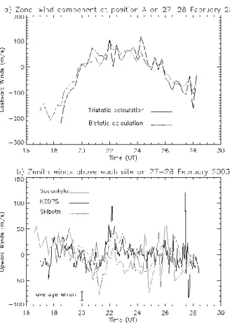
Fig. 2. (a) Comparison of zonal wind component calculated using
tristatic (all 3 FPIs) and bistatic (only KEOPS + Sodankyl¨a) line-of-sight measurements on the night of 27–28 February 2003. (b) Comparison of the vertical wind component observed by each of the 3 FPIs on the night of 27–28 February 2003.
deconvolved from the fringe profile in order to calibrate the FPI and determine an absolute temperature. Two of the FPIs, Skibotn and Sodankyl¨a, were absolutely calibrated using He-Ne laser profiles. As the KEOPS FPI was not absolutely cal-ibrated the measurements must be offset to produce agree-ment.
Neutral temperatures determined in this way may differ from the ambient thermospheric temperature if there is a significant contribution to the overall intensity from non-thermalised atomic oxygen. This would artificially increase the observed temperature, as demonstrated by Shematovich et al. (1999). Sipler and Biondi (2003), however, have shown that in their FPI Doppler temperature analysis, the contribu-tion of the non-thermalised component of the total emission was always less than 20 K, i.e. much less than their error estimates, for a range of solar activity conditions. Further, the main contribution to the temperature increase was from higher altitudes, above the peak emission height.
We have used the combination of instruments available for the current tristatic arrangement to demonstrate that for the majority of the time our peak altitude appeared to be close to our nominal 240-km peak height. This should ensure that we did not suffer from a significant contribution to the Doppler
temperature from non-thermalised emission. However, we are aware that the Sipler and Biondi (2003) conclusions were for mid-latitudes and that while the analysis techniques are essentially similar, the details may alter the impact of the non-thermal emission, so we are working to simulate these effects for our specific technique.
3 Meso-scale variability of the high-latitude thermo-sphere
3.1 Variability of thermospheric winds
Figure 2a shows the calculated zonal wind component for position A on the night of 27–28 February 2003. A compar-ison is made between the true tristatic calculation that uses the line-of-sight winds from all 3 FPIs and the bistatic cal-culation that uses the 2 FPIs with the highest time resolution (KEOPS and Sodankyl¨a). The bistatic calculation requires the assumption that the vertical wind component is zero to solve the equations. This is a commonly used assumption based on the observation that the vertical wind component is on average an order of magnitude smaller than the horizon-tal component. The discrepancy of up to 50 m/s between the tristatic and bistatic wind values is more due to the failure of this assumption rather than because the three FPIs are not ob-serving a common volume. Figure 2b shows the individual vertical components measured above each of the FPI sites. The location of the FPIs are such that Skibotn and KEOPS are at the same geographic longitude, separated by about 250 km, while KEOPS and Sodankyl¨a are at the same geo-graphic latitude, also separated by about 250 km. As noted earlier, the sensitivities of the FPIs were different, hence the various time resolutions. Inspection of the vertical wind plot shows that the winds were individually highly variable over this small area. The vertical winds ranged between ±50 m/s, with a few excursions to a maximum of 120 m/s upwards at 03:26 UT. The wind error is dependent on the signal-to-noise ratio, thus the vertical wind error bars were ±10 m/s up to midnight when the intensities were high. After midnight they rose to around ±20 m/s on average as the intensities became low.
The error due to a change in the peak emission height may be estimated by using the line-of-sight winds from the cardi-nal point observations, to determine the gradient of the wind field. Taking a possible extreme value, if the emission height was 50 km higher than 240 km and the line-of sight volumes over-reached position A, then the average change in the mag-nitude of the wind for this night would have been only around 10 m/s. Thus, the difference between the tristatic and bistatic calculations was mainly due to the vertical wind assumption. Similar trends in the nighttime variation of the vertical winds were seen independently in each of the data sets, es-pecially the large upwelling at 22:00 UT which was oc-curred when an auroral arc passed through this region. The vertical wind seen by both the KEOPS and Skibotn FPIs around this time rose sharply to around 100 m/s. Prior to the
upwelling, Skibotn showed strong downwelling to a maxi-mum of −78 m/s at 21:16 UT while KEOPS and Sodankyl¨a showed smaller downwelling during all or part of the period between 21:00–22:00 UT.
These are very large vertical winds but similar sized verti-cal winds at high latitudes have been reported by other work-ers (e.g. Price et al., 1995). Earlier observations were treated with scepticism, owing to the consideration of the large ener-gies required to move the atmosphere vertically. Shinagawa et al. (2003) carried out a modelling study of vertical winds generated by a moving auroral arc based on an EISCAT ex-periment. The study produced maximum vertical winds of 20 m/s which were less than the observed winds. This will be discussed in the section on ion-neutral coupling below.
The large upwelling resulted in a single data point indicat-ing a sharp drop of nearly 100±32 m/s in the tristatic zonal wind component at 22:00 UT. The tristatic winds were cal-culated with a resolution of 15 min, which is around the time taken for this rapid velocity spike to occur. However, the time resolution of the KEOPS line-of-sight measurements was far higher, as shown in Fig. 3. There were 6 data points between 21:54–22:12 UT from the KEOPS tristatic A measurements, with an error of ±16 m/s, which clearly show that this was a real geophysical observation rather than due to instrumental or observational error.
Conde and Smith (1998) show a similar drop in the hor-izontal wind field accompanying an upwelling which they have called the “doldrums”. They suggest that this is the re-sult of the advection of low velocity gas from the E-region up to the F-region. If this is the case, it might be expected that the upwelling gas package would carry E-region tempera-tures, but cooler due to adiabatic expansion. The radar mea-surements of Tiin the E-region were ∼500 K which would be
indicative of Tn at this altitude. The Sodankyl¨a FPI tristatic
A measurements showed no particular trends in Tn around
this time that might indicate the intrusion of an E-region gas parcel. The FPI measurements of neutral temperature are described in more detail in the temperatures section below. Furthermore, the main Joule heating at 22:00 UT was in the F-region where Ne and hence the conductivity was highest.
Thus, there would have been little reason for a gas parcel to rise to the hotter F-region altitudes from the E-region through buoyancy alone.
However, both the Sodankyl¨a tristatic A and North mea-surements of Tn showed a larger average Tn in the period
of the upwelling, i.e. <Tn>=1152 K (tristatic A) and 1132 K
(North) for the period 22:00–22:30 UT. This was followed by a drop in the average temperature to <Tn>=1062 K (tristatic
A) and 1045 K (North) for the period 22:30–23:00 UT fol-lowed by a rise back up to 1102 K (tri A) and 1078 K (North) for the period 23:00–23:30 UT. This temperature trend was also seen in the KEOPS tristatic A Tn measurements,
al-though the magnitudes involved are unresolved as the tem-peratures have not been calibrated. So it may be possi-ble that the drop in temperature can be interpreted as evi-dence of cooler E-region gas which took half an hour to cool the F-region by nearly 100 K. These temperature data are
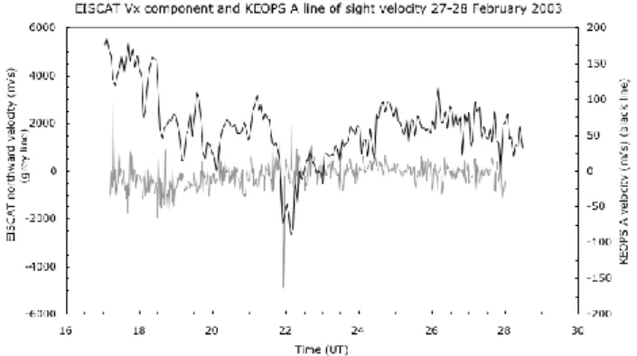
Fig. 3. Comparison of the EISCAT northward component of the
field-perpendicular ion velocity (left-hand scale) with the KEOPS FPI line-of-sight thermospheric wind (right-hand scale). The rapid thermospheric response to the ion velocity spike was largely due to a large upwelling caused by Joule heating as shown in Fig. 2b.
presented later in this paper under the section for ion-neutral coupling.
Alternately, instead of considering a dip in temperature around 23:30 UT, the temperatures around 22:00 UT and 23:00 UT could probably represent temperature rises due to heating and they do indeed match with peaks in the 630-nm intensities when there was particle precipitation.
The last evidence against the doldrums theory for explain-ing this behaviour comes from takexplain-ing all the KEOPS az-imuthal line-of-sight winds and calculating the horizontal wind field using the KEOPS zenith observation to give al-lowance for the vertical wind component. There does not appear to have been any distinct drop-off in speed that might indicate an upwelling from the E-region. Instead, this seems to have been a typical diverging wind field.
Figure 2b illustrates that the assumption of a zero ver-tical wind at any one time is not correct, however, over a whole night the assumption is adequate for determining a zero Doppler position. The reliability of this procedure depends on the geomagnetic activity during the night. As shown by Aruliah and Rees (1995), the average nighttime vertical wind is zero for geomagnetically quiet conditions, but tends to have a small upward value during active condi-tions when the auroral region suffers from sustained periods of upwelling due to Joule heating. This is likely to intro-duce a systematic offset of ∼5 m/s. So it is gratifying to see that the 3 independently calibrated FPIs showed simi-lar trends and variations in the vertical winds throughout the night despite sampling different regions of the upper atmo-sphere above each site. This indicates that the procedure used to determine the zero Doppler baseline is adequate.
Figure 3 shows that the large upwelling in the vertical wind around 22:00 UT corresponded to an extremely large and sudden increase in the ion velocity to around 5000 m/s for the northward component in the plane perpendicular to the magnetic field. The grey line shows the ion velocity V and the black line shows the neutral wind U . Note that the neutral
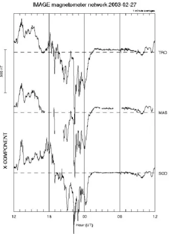
Fig. 4. IMAGE magnetometer traces from Tromsø, Masi and
So-dankyl¨a showing the Bxcomponent on the night of 27–28 February 2003 for a latitude range of 67◦–70◦N.
winds were an order of magnitude smaller than the ion veloc-ities. The ion velocity scale is to the left and the neutral wind scale to the right of the graph.
The neutral wind response to the sudden momentary ion velocity increase was more rapid than expected, although it was mainly in the vertical component rather than horizontal, as shown by Fig. 2b. It is interesting that the effect of this sudden increase lingered in the neutral winds for a few ten’s of minutes, as can be seen by the slow decline in the wind magnitude.
Price et al. (1995) have suggested that the sudden appear-ance of vertical winds may be caused by the advection of regions of upwelling into the field-of-view of their FPI rather than a sudden upward acceleration. It is possible that the si-multaneous surge in ion velocity and neutral wind upwelling observed in Fig. 3 may be a coincidence rather than a cause and effect. In order to test this it would be necessary to de-termine the vertical wind field over the region covered by the FPIs. However, our own observations and previous stud-ies (Crickmore, 1993) have already indicated that the scale size for the upper thermospheric vertical winds appears to be only a few 100 km in the auroral region. This makes us wary of extrapolating the zenith winds observed over the FPI
sites out to the edges of the viewing circles which have a pre-sumed radius of 240 km. However, the sudden increase and lingering decrease in the neutral wind seem more likely to be a response to a surge of ion drag forcing than a passing of region of upwelling, which might be expected to have a more smoothly varying effect. Another point is that the upwelling is seen simultaneously at both KEOPS and Skibotn, which lie along the same meridian. There is no indication of the possi-bility of a zonally travelling front of upwelling appearing at Sodankyl¨a, which is west of KEOPS, before (for a westward travelling front) or after (eastward) 22:00 UT. Further work arising from this experiment will combine modelling studies with these data to help resolve the issues uncovered.
The sudden increase in ion velocities was due to the pres-ence of high electric fields within auroral arcs during a sub-storm expansion. Figure 4 gives an indication of the geo-magnetic activity conditions on the night of 27–28 February 2003 by showing the perturbation of the Bx component of
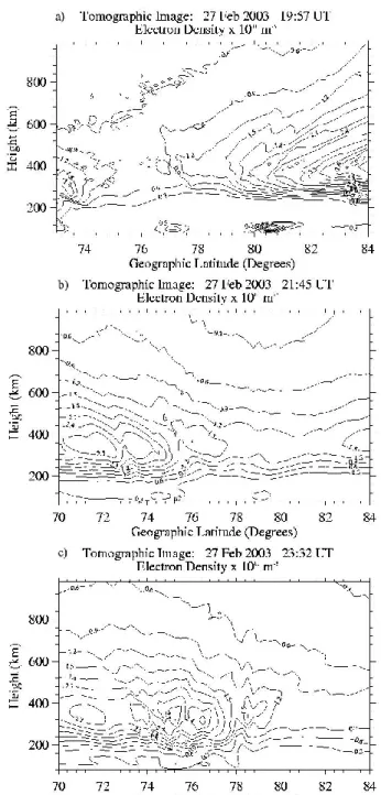
the geomagnetic field observed by the IMAGE magnetome-ter chain. The response of the general ionospheric electron density distribution to the increased geomagnetic activity is shown in the sequence of three tomographic images in Fig. 5. The first image at 19:57 UT (Fig. 5a), before the time of in-creased activity, shows the inin-creased electron densities of the auroral region in the northern field-of-view, with evidence of a boundary blob at the equatorward edge around 77–78◦N. By the next tomographic image at 21:45 UT (Fig. 5b) the au-roral structure was essentially south of 77◦N and extended to the low-latitude extreme of the field-of-view. A slight pole-ward retreat of the increased densities had occured by the tomographic image at 23:32 UT (Fig. 5c).
3.2 Ion-neutral coupling: first empirical confirmation of the importance of variability to Joule heating
It should be noted that average electric field models such as the Millstone Hill model (e.g. Foster, 1983) use average plasma velocities from the Millstone Hill radar smoothed over 2.5 h to calculate V ×B. A more recent electric field model by Weimer (1995) fits a spherical harmonic func-tion to binned satellite measurements. The consequence of such smoothed electric fields when used in GCMs is that too much momentum is transferred to the neutral gas at high lat-itudes, resulting in winds that are up to two times larger than measured by FPIs (Aruliah and Griffin, 2001; Griffin et al., 2004), and too little heat is generated, resulting in tempera-tures that are hundreds of Kelvin smaller than measured by FPIs (Killeen et al., 1995). This has already been recognised as a problem and Codrescu et al. (2000) have addressed the temperature discrepancy by calculating the variability of the Millstone Hill plasma velocities and adding this as a param-eter to the Foster average electric field model. However, it is proposed that Codrescu’s analysis of the standard deviation may be a major underestimate of Joule heating since:
1. The original radar velocities in the database are al-ready averaged over 2.5 h, as mentioned above, while
Fig. 5. Electron density tomographic images showing how the
au-roral oval expanded from (a) north of the FPIs’ field-of-view at 19:57 UT to (b) to south of 77◦N at 23:45 UT and then by (c) 23:32 UT retreating slightly poleward.
Lanchester et al. (1996) have shown variability down to resolutions of less than a second.
2. There is a spatial averaging over volumes that span a range of altitude and large horizontal range since the radar scan is a low-elevation, long range scan over hun-dreds of kilometres.
3. The binning of data according to geomagnetic and solar indices with coarse time resolution, such as Kp, which
Fig. 6. Comparison of the north and east components of the
mag-netospheric electric field (V ×B) using 1-min and 15-min averages with the neutral wind dynamo (U ×B) on the night of 27–28 Febru-ary 2003.
is a 3-h index, results in considerable smoothing. 4. The heating effect of particle precipitation should also
be considered. Satellite particle sensors with a finite time resolution, limited spectral energy resolution and range sample a complex 3-D pattern of precipitation via a 1-D cut over a limited geographic trajectory. These measurements are then converted into global particle precipitation models used in the GCMs. Although ex-tremely useful for climatology studies, they suffer from the limitation of being a low resolution spatial average of what are highly localised heating phenomena. Thus, small-scale heating effects are likely to be severely un-derestimated.
All the high-latitude electric field models ignore the neu-tral wind dynamo because at high latitudes the neuneu-tral wind dynamo, is assumed to be an order of magnitude smaller than the magnetospheric dynamo (e.g. Mozer, 1973). However, the neutral wind speeds in the upper atmosphere are an or-der of magnitude larger than in the E-region, owing to the reduced densities and consequently fewer collisions in the upper atmosphere, and can reach a few hundreds of m/s in magnitude (Killeen et al., 1995; Aruliah et al., 1996).
The plots in Fig. 6 show a comparison of the F-region neu-tral wind dynamo (U ×B) with the magnetospheric dynamo (V ×B). The magnetospheric dynamo field was calculated using both the 1-min average V and the 15-min average. The 1-min average V was large and highly variable while, obvi-ously, the 15-min average was fairly smoothly varying. The F-region neutral wind dynamo was also smoothly varying and had a magnitude that was significant in size compared with the 15-min average V ×B. The average magnitude of U ×B was 50% of V ×B during 27–28 February 2003, which is consistent with Killeen et al. (1984).
The important point of Fig. 6 is that the neutral wind had a steadily varying value through the night while the 1-min average values of the ion velocities had large erratic varia-tions. This is implied by the dynamo electric fields. The consequence is that the random nature of the ion velocities and therefore ion drag will produce a smaller acceleration of the neutral gas than predicted by model simulations that use steady-state electric fields.
Figure 7a shows the Skibotn and KEOPS FPI neutral tem-peratures at the tristatic A position which is presumed to be at an altitude of 240 km. These temperatures are com-pared with EISCAT ion temperatures at two altitudes 245 km and 294 km, for 27–28 February 2003. Figure 7b shows the corresponding Joule heating calculations. In particular, Fig. 7b shows the large difference introduced by including ionospheric variability into the calculation of Joule heating in the F-region. Thus, two sets of values representing Joule heating are plotted for the period 18:00–24:00 UT for the night of 27–28 February 2003. Joule heating is assumed to be proportional to Ne*E2perp, where Ne is the electron
den-sity, which represents the conductivity, and Eperpis the
mag-nitude of the electric field perpendicular to the magnetic field direction. The black and grey lines show the Joule heating term calculated using 15-min and 1-min averaged values, re-spectively, of V , to determine E=V ×B.
There was a dramatic difference between the Joule heat-ing calculated usheat-ing the 1-min and 15-min averages. There were six peaks (at 18:30 UT, 19:45 UT, 20:15 UT, 20:45 UT 22:00 UT and 23:30 UT) in Joule heating using the 1-min averages and only 3 peaks (at 20:45 UT, 22:00 UT and 22:45 UT) using the 15-min averages. The size of the 1-min average Joule heating term indicates that Joule heating can be grossly underestimated by ignoring the variability of the ion velocities. The median of the ratios of the 1-min to 15-min Joule heating measurements over the whole night is around 320%. Figure 7a shows that during the period 18:00– 19:00 UT the ion temperature rose sharply from 1200 K to over 1600 K before dropping quickly down. This seems to show a clear correspondence with a peak in the 1-min Joule heating term (Fig. 7b), while there was no corresponding in-crease in the 15-min Joule heating term.
What is interesting is that there does not appear to be such a clear correspondence between Joule heating and Ti for the
subsequent peaks. However, we would suggest that this is due to the breakdown of the assumptions used to calculate Ti for the period 20:00–24:00 UT, resulting in anomalous
Fig. 7. (a) Comparison of Sodankyl¨a FPI measurements of Tn at tristatic A and North look directions with EISCAT Tiat altitudes of 245 km and 294 km for the period 18:00–24:00 UT on the night of 27–28 February 2003. (b) Illustrating the importance of meso-scale ion velocity variability for determining Joule heating by comparing 1-min and 15-min average values for the same period as Fig. 7a. The periods of F-region intensifications of electron density are indicated by grey panels on Figs. 7a and b.
temperatures. This is discussed in the following section about temperatures.
Further support for the importance of mesoscale variabil-ity is that the period of large Joule heating values between 21:30–22:30 UT corresponded to high vertical winds of up to 100 m/s, seen independently by the KEOPS and Skibotn FPIs. As stated previously, Shinagawa et al. (2003) car-ried out a modelling study of vertical winds generated by a moving auroral arc based on an EISCAT experiment by Oyama et al. (2001). The study produced maximum verti-cal winds of 20 m/s, which were considerably less than the observations, and the authors acknowledge the need for a larger energy flux. The sample frequency for their electric fields appears from their figures to have been 2 s. Yet the variability does not appear to be as large as for our 1-min
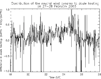
Fig. 7. (c) Percentage contribution of the neutral wind dynamo to
Joule heating on the night of 27–28 February 2003.
Fig. 7. (d) EISCAT Ne, Ti, Teand V data for the period 18:00– 24:00 UT on 27–28 February 2003. The periods of F-region inten-sifications of electron density are indicated by arrows.
radar measurements, which may imply that their data have been smoothed. Our observations suggest that large vertical winds may occur at intervals of high-temporal variation in Joule heating. This was not explored in the modelling study of Oyama et al. (2001). Our experiment appears to provide the first evidence that meso-scale variability must be taken into account when calculating Joule heating.
The Sodankyl¨a thermospheric temperature response shown in figure 7a differed from the ion temperatures. This is as expected since the neutral particle number density is 3 orders of magnitude larger, thus the thermosphere has a considerably larger heat capacity. There was no apparent re-sponse in Tnto the first heating event between 18:00–19:00
UT. However, Tn rose steeply by 200 K between 19:20–
19:40 UT, fell sharply and rose again, reaching a maximum
Fig. 7. (e) Deducing the thermospheric temperature difference
along the radar beam from KEOPS FPI North and tristatic A mea-surements for the period 18:00–24:00 UT on 27–28 February 2003.
value of 1230 K around 20:30 UT. The neutral temperature then decreased, with several fluctuations, by around 250 K over 3.5 h. In general, higher values of Tn existed after
19:30 UT which seem consistent with the period of enhanced Joule heating calculated using the 1-min average Joule heat-ing values shown in Fig. 7b.
A further comment is that Joule heating should be calcu-lated in the frame of reference of the neutral wind, which means that the effective electric field is E0=V ×B+U ×B.
Figure 7c shows the percentage difference made by the neutral wind dynamo in calculating the Joule heating term. This percentage difference is calculated using (E0perp2 −Eperp2 )/Eperp02 and has both positive and negative values, i.e. the effect of the neutral wind dynamo was to both enhance and reduce magnetospheric Joule heating. The standard deviation of the percentage difference for the 1-min averaged data ranges was 49% on this night (with sev-eral outliers that are extremely large). The net effect for the night of 27–28 February was an 8% increase in Joule heat-ing. However, the size of the neutral wind dynamo contribu-tion can be appreciated by calculating the average magnitude |Eperp02 −Eperp2 )/E0perp2 |of the neutral wind dynamo contri-bution to total Joule heating on this night, which was 29%. This is consistent with a model study by Thayer et al. (1995) that has shown that ignoring the flywheel effect can intro-duce a 40% error in the calculation of height-integrated polar cap Joule heating during steady-state moderately active con-ditions. Thus, ignoring the neutral wind dynamo means that the redistribution of magnetospheric energy between Joule heating and acceleration of the thermosphere can be mistaken by several tens of percent. This is in addition to the effect of highly variable ion velocities compared with steady-state model conditions in increasing Joule heating and reducing the net momentum transfer to the neutral winds.
Figure 7d shows panel plots of the electron densities, Ne,
Fig. 8. (a) Comparison of thermospheric temperatures from
inde-pendent measurements of a common volume by 3 FPIs on the night of 28 February–1 March 2003. (b) Comparison of the normalised intensities from the 3 FPIs for this night.
Fig. 9. IMAGE magnetometer traces showing the Bxcomponent on the night of 28 February–1 March 2003 at Sodankyl¨a.
and V . Between 22:00–23:00 UT it was necessary to move the Tromsø beam to a position 300 km above tristatic A, in order to improve the signal. This is shown in Fig. 7d as a shift in all the panel plots to a higher altitude range. There were 4 periods of E-region particle precipitation that can be observed in Fig. 7d from the enhancement of Ne
around 100–150 km altitude. The E-region particle precipita-tion was sporadic and occurred over periods between approx-imately 18:00–18:45 UT, 20:00–20:45 UT, 22:00–22:30 UT and 23:00–23:30 UT. The peaks in in-situ F-region Joule heating calculated using 1-min averages do not match the periods of E-region particle precipitation. In fact, the peri-ods of particle precipitation generally encompassed the low-est values of Joule heating. However, the Joule heating peaks do match intensifications of the electron densities in the F-region, i.e. in the periods 20:30–21:00 UT, 21:15–22:15 UT and 23:15–24:00 UT, as shown in Fig. 7d. These periods are indicated on Figs. 7a and b by grey panels, and on Fig. 7d by arrows. These F-region intensifications may arise from low-energy particle precipitation and also composition changes affecting production and loss of electrons, as well as equa-torward transport of electrons from the polar cap.
3.3 Tristatic neutral temperatures and anomalous ion tem-peratures
Thermospheric neutral temperatures are an important mea-sure of the energetics of the upper atmosphere. Given their importance, it is necessary first of all to establish the re-liability of the temperature measurements from the FPIs. Figure 8a compares the derived neutral temperatures from the three FPIs at tristatic position A on the second night (28 February until 1 March 2003). The Skibotn and So-dankyl¨a temperatures were absolutely calibrated using a He-Ne laser and ranged between 700–1400 K, with an average
error of ±50 K. These represent the first reported compar-isons of independently calibrated absolute temperature mea-surements from a common thermospheric volume. The grey lines represent the Sodankyl¨a data and the open diamonds represent the Skibotn data. The black lines represent the un-calibrated KEOPS data, which have been offset by a constant value to match Sodankyl¨a in order to compare trends.
The Skibotn temperatures have been filtered to exclude cloudy conditions identified from all-sky camera observa-tions, and have also had profiles removed that were af-fected by CCD saturation. The remaining periods around 21:00–22:00 UT and during 02:00–03:00 UT on the night of 28 February–1 March 2003 demonstrate good agreement between the 3 sets of temperatures. The 630-nm intensities at the 3 sites showed a close match (Fig. 8b). This may be interpreted as all 3 FPIs observing the same volume. The comparison also revealed a large degree of temporal struc-ture that appeared in all three sets of measurements. The time resolution at KEOPS was over two times better than that at Sodankyl¨a and showed a great deal of small-scale temporal variation. When viewed in conjunction with the Sodankyl¨a magnetometer data presented in Fig. 9 it is clear that the large increases in temperature after 18:00 UT and again after 22:00 UT coincided with large negative Bx
de-flections and consequent electrojet activity. There was no evidence of a substantial time lag between the observation of the magnetometer deflections and the resultant increase in
Fig. 10. (a) A close-up of the Sodankyl¨a thermospheric
tempera-ture gradients from 18:00–22:00 UT on the night of 28 February– 01March 2003. (b) The Sodankyl¨a 630-nm intensities over the same period. (c) The average magnitude of the horizontal wind component calculated from the 4 cardinal directions from the So-dankyl¨a FPI over the same period.
neutral temperature, thereby demonstrating a rapid thermo-spheric response.
The good agreement between the calibrated temperatures from Sodankyl¨a and Skibotn in Fig. 8a would imply either that the two FPIs were measuring a common volume, or that the spatial variability of the neutral temperature was small. If the spatial variability of Tnwas small, then even if there had
been a rise in the emission height (which would mean that the FPIs were overshooting the common volume) the 3 separate measured values would still agree.
Fig. 11. Electron density tomographic images at 22:46 UT on 28
February 2003 showing that enhanced densities that were associ-ated with the auroral activity extended to latitudes equatorward of Sodankyl¨a. The arrow indicates the latitude of the tristatic A posi-tion.
However, in fact, there were sizeable meridional temper-ature differences over the field-of-view of 200–400 K be-tween 16:00–21:00 UT on the night of 28 February–1 March 2003. Figure 10a focuses on showing the neutral temper-atures for the period 18:00–22:00 UT from the Sodankyl¨a North, Zenith, tristatic A and bistatic B observation points. The North and A values of Tn were similar to each other,
but significantly different from the Zenith and B values. The variation of the meridional temperature difference may be further investigated by comparing the temperatures observed to the north and south of Sodankyl¨a for the period 18:50– 20:10 UT. This gives an overall average meridional temper-ature difference of 270 K, with a maximum difference of 466 K at 19:16 UT.
Figure 10b shows the corresponding intensities and Fig. 10c shows the average magnitude of the horizontal wind component calculated from the 4 cardinal directions from the Sodankyl¨a FPI. It is clear that before 20:00 UT the auroral ac-tivity was to the north of Sodankyl¨a, resulting in the larger in-tensities seen in the North and A positions. The large merid-ional gradient in temperature would appear to have been a consequence of auroral heating to the north. From 22:30 UT onwards, the auroral activity moved overhead, and the in-tensities and temperatures became more uniform. The to-mography plot of electron density at 22:46 UT (Fig. 11) con-firms this by showing that enhanced densities associated with the auroral activity extended to latitudes equatorward of So-dankyl¨a.
It is also possible that the sharp increase and decrease in the temperature gradient may have been the consequence of a rise in the 630-nm emission height. If it is assumed that the temperature gradient remained constant but that the emis-sion height had risen, then the emitting volumes seen by the FPI to the north and south of Sodankyl¨a would have been further apart, which could account for the increase in
tem-perature gradient. However, the emission height would need to rise by 70% to produce such a large increase in the tem-perature gradient. This is too large a rise to be plausible over a horizontal scale of several hundred kilometres, since the energy required to lift the atmosphere would be very great. Another argument against a rise in the emission altitude is that the North and tristatic A intensities and temperatures re-mained close in values throughout this period. A rise in alti-tude would have meant that their respective sampled volumes would have consequently spread apart and the values would have become different.
Figure 10c shows that before 22:00 UT the magnitudes of the horizontal wind were high and ranged between 200–300 m/s. In particular, between 18:45–1930 UT the magnitudes were nearly 300 m/s. The large size of these winds probably corroborates the existence of a large tem-perature gradient and consequently large pressure gradient driving these winds.
The absolute calibration of the Sodankyl¨a temperatures al-lows a further important observation to be made. Going back to the first night of observations on the night of 27–28 Febru-ary 2003, a comparison of Tnfrom the Sodankyl¨a FPI with
Ti calculated from the EISCAT data for a height of 245 km
(Fig. 7a) showed an anomaly in Ti – there was an extended
period between 19:50–22:40 UT when Ti<Tn. The
reliabil-ity of the measurement of Tn comes from the comparison
with the independent measurements of Tnfrom the other two
FPIs. Therefore, these values of Ti are unlikely to be correct
since the ionosphere is less than 0.1% of the composition of the upper atmosphere, and consequently, through ion-neutral collisions, the ion temperatures must be at least as high as the neutral temperature. One possible error in the computation of Ti arises from the assumption of a composition that is
to-tally atomic oxygen and the other is that the radar spectra are non-Maxwellian and consequently not fitted appropriately.
The evidence for changing the composition is ambiguous. The period between 21:20–22:20 UT corresponded to a large upwelling in the neutral winds, as shown in Fig. 2b, which may have increased the proportion of molecular species at this height. However, the period between 20:00–20:40 UT corresponded to downwelling in the neutral winds, which would be unlikely to change the mean molecular mass and therefore does not provide enough support for the composi-tion theory.
The suggestion that Ti is incorrectly calculated is
sup-ported by Fig. 7d. Whenever there was precipitation in the F-region (around 400 km) the electron temperature Tedropped
by a few hundred Kelvin. This is clearly evident in the 2 periods centred on 19:16 UT and 19:37 UT and the pe-riods: 20:27–20:48 UT, 21:35–21:53 UT, 22:00–22:19 UT and 23:50–24:00 UT. Despite the increased electron densi-ties caused by precipitation, which would have increased the conductivity and hence Joule heating, Te should have
re-mained fairly constant since electron heating is very small and is primarily due to plasma wave activity (e.g. Schlegel and St.-Maurice, 1981). The implication is that the standard procedure for determining Te is incorrect, and thus Ti will
Fig. 12. Variation of hmF2 on the nights of (a) 27–28 February 2003
and (b) 28 February–1 March 2003 from EISCAT and tomography data. It is assumed that the 630-nm peak emission height is 240 km (dot-dashed line). This assumption is compared with an assumption that the peak height is about 50 km below hmF2 (dotted line).
be wrongly calculated too since Ti/Te is the parameter
de-termined from the radar spectra. Anomalous decreases in Te
have been proposed as a flag indicating incorrect assump-tions of composition or the presence of non-Maxwellian radar spectra by McCrea et al. (1995).
If the Ti values were correctly calculated, then a
possi-ble cause for the anomalous Ti–Tn comparison arises from
the height variation of the red line peak emission altitude. Figure 7a also shows the EISCAT Ti at 294 km altitude.
Comparison of Ti at 245 km and 294 km shows that before
20:00 UT there was only a small difference in Ti (<100 K)
with respect to height, so determination of the altitude of the common volume is not critical. After 20:00 UT there was a large difference, up to a maximum of 400 K, which means the altitude used for comparison of Tnand Ti becomes very
sensitive. At 294 km there were no longer anomalous peri-ods when Ti<Tnwhich may imply that this altitude provides
a more likely common volume. The tristatic experiment as-sumes a common volume at an altitude of 240 km. However, Fig. 12a shows that between 20:00–20:40 UT hmF2 rose to an altitude of around 350 km, and between 21:20–22:00 UT
the altitude was around 375 km. Thus, an altitude of 300 km may be acceptable as the altitude of the 630-nm emission peak if it is assumed that the peak is one scale height be-low the hmF2 peak, although this is considerably higher than expected.
If the Tivalues are correct, then an explanation is required
for the large difference in Ti measured at altitudes 245 km
and 294 km that appeared after 20:00 UT. This time corre-sponded to a switch in the line-of-sight ion velocities from blue shifted (NWW direction) to red shifted (SEE direction), as shown in Fig. 7d. This may indicate that the heat energy was being transported up the field lines so that the F-region remained hot while the lower altitudes cooled. However, this explanation does not address the extremely low temperatures at 245 km after 20:00 UT, which reached as low as 800 K.
The radar data from 245 km and 294 km represents a hori-zontal as well as vertical spatial difference since the elevation angle of the Tromsø beam is 45◦. This means that compar-ison may be made with FPI measurements from other view-ing directions, in particular a comparison of the KEOPS FPI Tn to the north of KEOPS with the KEOPS Tn at position
A. The difference between the two temperatures is an indi-cation of the thermospheric temperature gradient along the Tromsø beam (see Fig. 1) and will define the minimum pos-sible value of Ti along the beam. Figure 7e shows that the
temperature difference was rarely more than ±200 K. Dur-ing the period 20:00–24:00 UT, not only was the Tn
differ-ence much smaller than the Ti difference, but it was in the
wrong direction, since Tnto the north of KEOPS was on
av-erage hotter. This casts further doubt on the reliability of the values of Tiat 245 km.
Resolving the cause of these anomalies is our next venture; it is either the influence of increased molecular ion compo-sition or non-Maxwellian spectra in the EISCAT data; deter-mining or what altitude should be used for the comparison of Ti and Tnis also increasing. Furthermore, tristatic common
volume experiments are the most likely way to achieve this. 3.4 Variation of the 630-nm peak emission altitude The EISCAT volume of observation is known since it is an active radar, but passive airglow observation depends on the 630-nm peak emission height, which is assumed to be 240 km (e.g. Solomon et al., 1988). However, if the 630-nm emission height is different, then the FPIs over/undershoot the tristatic volume. It should be possible to estimate the height of the 630 nm emission from the EISCAT measure-ment of hmF2, since it is assumed to be approximately 1 scale height (40–50 km) below hmF2 (e.g. Makela et al., 2001). Figure 12 shows that there was considerable devi-ation from this assumption by plotting hmF2 for the two campaign nights, 27–28 February 2003 and 28 February–1 March 2003. The values of hmF2 are greater than 300 km for most of both nights, which implies that the FPIs were over-shooting the common volume for significant periods.
The height of the F2 peak obtained by radio tomography at a latitude of 70◦N is shown by the asterisks in Fig. 12. The
tomography heights are in broad agreement with the trend seen in the hmF2 measured by the EISCAT radar, though with a lower peak height occurring between about 02:00 and 04:00 UT. Whilst there is clear agreement in the trend, the absolute values of the peak altitudes inferred from the tomo-graphic images should be treated with some caution due to the incomplete observing ray-path geometry for the experi-mental technique. The lack of quasi-horizontal ray-paths re-sults in limited information of the vertical ionospheric distri-bution being available for the reconstruction process (Pryse, 2003).
Despite the likely variation in the 630-nm peak height throughout the night, the independently measured intensi-ties from the 3 FPIs matched very well on the 2 campaign nights of 27–28 February and 28 February–1 March 2003 (Figs. 13b and c). In contrast, the night of 26–27 Febru-ary (Fig. 13a) showed the effect of light scatter by clouds over Sodankyl¨a and Skibotn through the night. Cloud scat-ter raises the whole background level, thus reducing the signal-to-noise ratio and also the directional information is lost, resulting in a poor match in intensities. However, by 03:00 UT the cloud had cleared and so the Sodankyl¨a in-tensities rose to match the KEOPS inin-tensities. The Skibotn intensities matched KEOPS well from the beginning of the night through to about 21:45 UT, after which the sky became overcast and the intensities dropped.
The assumption of a peak 630-nm emission altitude of 240 km can be further tested by taking advantage of the tristatic geometry and complementary instrumentation in the region. In Fig. 14 we present a comparison of the 630-nm intensity for a 2-h period from 21:30 UT to 23:30 UT on 27–28 February 2003 as measured by the Sodankyl¨a and KEOPS FPIs, together with a Meridian Scanning Photome-ter (MSP) co-located with the Sodankyl¨a FPI. The intensities have been arbitrarily scaled to allow for a comparison of the major features. The MSP was oriented azimuthally towards the tristatic volume for the duration of the tristatic experi-ment and scanned from elevations of 20◦–75◦. The figure shows the MSP intensities at 45◦elevation, which was the same as the elevation angle of the Sodankyl¨a FPI. These in-tensities are compared to both the KEOPS tristatic and the Sodankyl¨a North intensities. The reason for the comparison with Sodankyl¨a North intensities is that if the peak emission altitude had been 300 km, rather than 240 km, then the vol-ume observed by KEOPS would have been much closer to Sodankyl¨a North than to the Sodankyl¨a tristatic position (see Fig. 1 for geometry). Figure 14 shows a close agreement between the KEOPS FPI tristatic A observation and the So-dankyl¨a MSP measurements which consequently gives con-fidence that the peak emission altitude was closer to 240 km than 300 km.
Unfortunately, this contradicts the suggestion that the problem of the anomalous ion temperatures period (when Ti<Tnaround 240 km altitude) may be solved by presuming
Fig. 13. Comparison of intensities from the 3 FPIs on 3 consecutive
nights: (a) 26–27 February 2003, (b) 27–28 February 2003 and (c) 28 February–1 March 2003.
Fig. 14. Investigation of the 630-nm emission height by
compari-son of features seen by the Sodankyl¨a MSP with the KEOPS and Sodankyl¨a FPIs on the night of 27–28 February 2003.
4 Preliminary conclusions
This tristatic FPI-EISCAT radar experiment presents evi-dence of the rapid response of the thermosphere to ion drag on the meso-scale. High temporal variability in thermo-spheric temperatures and winds are demonstrated, which
varied significantly over time scales of a few minutes and over distances of a few hundred kilometres. As a result, the prevailing view of the inertial thermosphere can no longer be justified on the meso-scale, except as the coarsest of assump-tions, and certainly not in storm situations.
The tristatic FPI measurements present the first ever com-parison of absolute temperatures from independently cali-brated FPIs. True thermospheric temperatures are vitally im-portant as a measure of the energetics of the upper atmo-sphere. The FPIs provided direct measurements of Tnrather
than derived values from radar measurements which rely on assumptions from models. The 3 different line-of-sight mea-surements showed a good agreement which confirms the re-liability of the experimental method in determining absolute temperatures.
The most significant finding is that the neutral and ion tem-perature response appears to have a better match with Joule heating calculated from the highly variable 1-min plasma ve-locities rather than 15-min averages for the night of 27–28 February 2003. There was a 320% increase in the Joule heat-ing when usheat-ing the 1-min average ion velocities compared with the 15-min averages, owing to the stochastic motion of the ions which increases friction between the ions and neu-trals. This is the first direct evidence of the effect of small-scale variability on Joule heating. It is important because the current GCMs ignore small-scale variability, and thus under-estimate Joule heating, by using smoothed high-latitude av-erage electric field models. This would account for the low model temperatures which can be hundreds of Kelvin lower than observed directly by FPIs and the low model vertical winds (<20 m/s) which are several times smaller than ob-served. It has taken many years for the observations of large vertical winds (>50 m/s) to be taken seriously.
The interpretation of the Joule heating-temperature rela-tionship is complicated by an extended period of anomalous ion temperatures when Ti<Tn. However, we propose that
the anomaly indicates flaws in the assumptions used in de-riving Ti, possibly due to the existence of non-Maxwellian
spectra, incorrect assumptions of the molecular ion compo-sition or misidentification of the height of the common vol-ume. The height is not thought to be the problem because comparison between auroral features observed in FPI inten-sities and meridian scanning photometers seem to indicate that the 630-nm emission height does not stray too far from 240 km.
Further support for the inclusion of the variability of the plasma velocities in GCMs is that it should also reduce the net momentum transferred from the ions to the neutrals, re-sulting in smaller neutral winds. This would improve agree-ment with the wind speeds measured by FPIs. Model winds at high latitudes can be up to twice as large as observed winds. However, the discrepancy between observations and models in allocating magnetospheric energy between Joule heating and acceleration of the neutral gas is too complex to be resolved by a simple transfer of energy from one form to the other. For example, as a rough order of magnitude cal-culation, the difference in kinetic energy between a model
wind of 300 m/s and FPI wind of 200 m/s corresponds to a temperature difference of only 30–40 K, which is not enough to account for the model neutral temperatures being a few hundred Kelvin lower than the FPI temperatures. The reduc-tion in the model winds needs to be brought about by allow-ing for a random stochastic acceleration of the neutrals rather than a steady acceleration. This can probably be achieved by parameterization in a similar manner to that used for Joule heating by Codrescu et al. (2000).
The F-region neutral wind dynamo has been shown to be around half the magnitude of the 15-min average magneto-spheric dynamo. This also significantly modifies the redistri-bution of magnetospheric energy between Joule heating and acceleration of the thermospheric gas. The study of small-scale ion-neutral interactions is proving to be extremely com-plex.
Appendix A
Theoretically, the derivation of a tristatic wind vector may be achieved by setting up and solving the simultaneous equa-tions for the 3 line-of-sight measurements in the following manner:
Let the neutral wind vector be U =Uxi+Uyj + Uzk.
And the direction vector for the line-of-sight observation be r= sin θ cos φi+ sin θ sin φj+ cos θ k, where i, j and k are orthogonal axes with positive directions being geographic north, geographic east and vertically down, respectively. The angles θ and φ are the standard spherical coordinate system definitions, i.e. θ is measured from the k axis and φ lies in the i, j plane and is measured from the i axis.
Thus the line-of-sight component winds Ulos from each
site may be determined from the following equations:
Uglos =U .rg for KEOPS
Uf los =U .rf for Sodankyl¨a
Umlos =U .rm for Skibotn .
These 3 equations may be given in matrix form as
Ulos=R.U. Thus, U=R−1Ulos.
The success of this calculation requires good geometry and the assumption that all three line-of-sight wind measure-ments come from the same volume. The optimal geometry is that the 3 sites and the observed volume form an equilateral pyramid. The observation of a common volume depends on the actual height of the 630-nm emission peak, which for this experiment was expected to be 240 km.
Acknowledgements. The APL team would like to acknowledge
funding from the Lapbiat grant, administered by the Sodankyl¨a Geophysical Observatory, together with their generous help in lo-gistics. Also acknowledging PPARC grant PPA/G/O/2001/00484. EISCAT is an International Association supported by Finland (SA), France (CNRS), the Federal Republic of Germany (MPG), Japan (NIPR), Norway (NFR), Sweden (NFR) and the United Kingdom (PPARC). We also thank the institutes who maintain the IMAGE magnetometer array and ESRANGE KEOPS facility.
Topical Editor M. Lester thanks M. Conde and another referee for their help in evaluating this paper.
References
Aruliah, A. L. and Rees, D.: The trouble with vertical winds: Ge-omagnetic, seasonal and solar cycle variations in high latitude thermospheric winds, J. Atmos. Terr. Phys., 57, 597–609, 1995. Aruliah, A. L., Farmer, A. D., Rees, D., and Brandstrøm, U.: The
seasonal behaviour of high latitude thermospheric winds and plasma velocities observed over one solar cycle, J. Geophys. Res., 101, 15 701–15 711, 1996.
Aruliah, A. L., and Griffin, E. M.: Meso-scale structure in the high-latitude thermosphere, Ann. Geophys., 19, 37-46, 2001. Aruliah, A. L., M¨ullerWodarg, I. C. F., and Schoendorf, J.: The
con-sequences of geomagnetic history on the high-latitude thermo-sphere and ionothermo-sphere: Averages, J. Geophys. Res., 104, 28 073– 28 088, 1999.
Aruliah, A. L., Griffin, E. M., McWhirter, I., Aylward, A. D., Ford, E. A. K., Charalambous, A., Kosch, M. J., Davis, C. J., and How-ells, V. S. C.: First tristatic studies of meso-scale ion- neutral dynamics and energetics in the high-latitude upper atmosphere using co-located FPIs and EISCAT radar, Geophys. Res. Lett., 31, L03802, doi:10.1029/2003GL018469, 2004.
Bilitza, D.: International Reference Ionosphere-Status 1995–1996, Adv.Space Sci., 20, 1751–1754, 1997.
Cierpka, K., Kosch, M. J., Rietveld, M., Schlegel, K., Hagfors, T.: Ion-neutral coupling in the high-latitude F-layer from incoherent scatter and Fabry-Perot interferometer measurements, Ann. Geo-phys., 18, 1145–1153, 2000,
SRef-ID: 1432-0576/ag/2000-18-1145.
Conde, M. and Smith, R. W.: Spatial structure in the thermospheric horizontal wind above Poker Flat, Alaska, during solar mini-mum, J. Geophys. Res., 103, 9449–9471, 1998.
Conde, M., Craven, J. D., Immel, T., Hoch, E., Stenbaek-Nielson, H., Hallinan, T., Smith, R. W., Olson, J., Sun, Wei, Frank, L. A., and Sigwarth, J.: Assimilated observations of thermospheric winds, the aurora, and ionospheric currents over Alaska, J. Geo-phys. Res., 106, 10 493–10 508, 2001.
Codrescu, M. V., Fuller-Rowell, T. J., Foster, J. C., Holt, J. M., and Cariglia, S. J.: Electric field variability associated with the Millstone Hill electric field model, J. Geophys. Res., 105, 5265– 5273, 2000.
Crickmore, R. I.: A comparison between vertical winds and diver-gence in the high-latitude thermosphere, Ann. Geophys., 11, no. 8, 728–733, 1993.
Etemadi, A., Cowley, S. W. H., and Lockwood, M.: The effect of rapid changes in ionospheric flow on velocity vectors deduced from radar beam-swinging experiments, J. Atmos. Terr. Phys., 51, 125–138, 1989.
Foster, J. C.: An empirical electric field model derived from Chatanika radar data, J. Geophys. Res., 88, 981–987, 1983. Greet, P. A., Conde, M. G., Dyson, P. L., Innis, J. L., Breed, A.
M., and Murphy, D. J.: Thermospheric wind field over Mawson and Davis, Antarctica: simultaneous observations by two Fabry-Perot spectrometers of 630 nm emission, J. Atmos. Terr. Phys, 61, 1025–1045, 1999.
Griffin, E. M., Aruliah, A. L., M¨uller-Wodarg, I. C. F., and Ayl-ward, A. D.: Comparison of high-latitude thermospheric merid-ional winds I: Optical and radar experimental comparisons, Ann. Geophys., 22, 849–862, 2004,
SRef-ID: 1432-0576/ag/2004-22-849.
Innis, J. L. and Conde, M.: High-latitude thermospheric vertical wind activity from Dynamics Explorer 2 Wind and Tempera-ture Spectrometer observations: Indications of a source region
for polar cap gravity waves, J. Geophys. Res, 107, Issue A8, SIA 11-1, CiteID 1172, doi:10.1029/2001JA009130, 2002.
Ishii, M., Conde, M., Smith, R. W., Krynicki, M., Sagawa, E., and Watari, S.: Vertical wind observations with two Fabry-Perot interferometers at Poker Flat Alaska, J. Geophys. Res, 106, 10 537–10 551, 2001.
Killeen, T. L., Hays, P. B., Carignan, G. R., Heelis, R. A., Hanson, W. B., Spencer, N. W., and Brace, L. H.: Ion-Neutral Coupling in the High Latitude F-Region: Evaluation of Ion Heating Terms from Dynamics Explorer 2, J. Geophys. Res., 89, 7495–7508, 1984.
Killeen, T. L., Won, Y. -I., Niciejewski, R. J., and Burns, A. G.: Up-per Thermosphere Winds and TemUp-peratures in the Geomagnetic Polar Cap: Solar Cycle, Geomagnetic Activity and IMF Depen-dencies, J. Geophys. Res., 100, 21 327–21 342, 1995.
Lanchester, B. S., Kaila, K., and McCrea, I. W.: Relationship be-tween large horizontal electric fields and auroral arc elements, J. Geophys. Res., 101, 5075–5084, 1996.
Lockwood, M., Cowley, S. W. H., Smith, M. F., Rijnbeek, R. P., and Elphic, R.C.: The contribution of flux transfer events to convec-tion, Geophys. Res. Lett., 22, 1185–1188, 1995.
Makela, J. J., Kelley, M. C., Gonzalez, S. A., Aponte, N., and Mc-Coy, R. P.: Ionospheric topography maps using multiple wave-length all-sky images, J. Geophys. Res., 106, 29 175–29 184, 2001.
McCrea, I. W., Jones, G. O. L., and Lester, M.: The BEAN experi-ment – An EISCAT study of ion temperature anisotropies, Ann. Geophys., 13, 177–188, 1995,
SRef-ID: 1432-0576/ag/1995-13-177.
Millward, G. H., Moffett, R. J., Quegan, S., and Fuller-Rowell, T. J.: A coupled thermosphere-ionosphere-plasmasphere model (CTIP), STEP Handbook of ionospheric models, edited by Schunk, R. W., 1996.
Mozer, F. S.: Analysis of Techniques for Measuring DC and AC Electric Fields in the Magnetosphere, Space Sci. Rev, 14, 272– 313, 1973.
Oyama, S., Ishii, M., Murayama, Y., Shinagawa, H., Nozawa, S., Buchert, S. C., Fujii, R., and Kofman, W.: Generation of atmo-spheric gravity waves associated with auroral activity in the polar F-region, J. Geophys. Res., 106, 18 543–18 554, 2001.
Picone, J. M., Hedin, A. E., Drob, D. P., and Aikin, A. C.: NRLMSISE-00 empirical model of the atmosphere: Statistical comparisons and scientific issues, J. Geophys. Res, 107(A12), 1468, doi:10.1029/202JA009430, 2002.
Price, G. D., Smith, R. W., and Hernandez, G.: Simultaneous mea-surements of large vertical winds in the upper and lower thermo-sphere, J. Atmos. Terr. Phys. 57, 631–643, 1995.
Pryse, S. E.: Radio tomography: a new experimental technique, Surveys in Geophysics, 24, 1–38, 2003.
Rishbeth, H. and Williams, P. J. S.: The EISCAT Ionospheric Radar: the System and its Early Results, Q. Jl. R. Astr. Soc., 26, 478– 512, 1985.
Sakonoi, T., Fukunishi, H., Okano, S., Sato, N., Yamagishi, H., and Yukimatu, A.: Dynamical coupling of neutrals and ions in the high-latitude F-region: Simultaneous FPI and HF radar observa-tions at Syowa Station, Antarctica, J. Geophys. Res., 107, A11, doi:10.1029/2001JA007530, 2002.
Schlegel, K., and St.-Maurice, J. P.: Anomalous heating of the polar E region by unstable plasma waves 1. Observations, J. Geophys. Res., 86, 1447–1452, 1981.
Shematovich, V., Gerard, J.-C., Bisikalo, D. V., and Hubert, B.: Thermalization of O(1D) atoms in the thermosphere, J. Geophys. Res., 104, 4287–4295, 1999.
Shinagawa, H., Oyama, S., Nozawa, S., Buchert, S. C., Fujii, R., and Ishii, M.: Thermospheric and ionospheric dynamics in the auroral region, Adv. Space Res., 31, 951–956, 2003.
Sipler, D. P. and Biondi, M. A.: Simulation of hot oxy-gen effects on ground-based Fabry-Perot determinations of thermospheric temperatures, J. Geophys. Res., 108, A6, doi:10.1029/2003JA009911, 2003.
Solomon, S. C., Hays, P. B., and Abreu, V. J.: The auroral 6300A emission: Observations and modeling, J. Geophys.Res., 93, 9867–9882, 1988.
Thayer, J. P., Vickrey, J. F., Heelis, R. A., and Gary, J. B.: Interpre-tation and modelling of the high-latitude electromagnetic energy flux, J. Geophys. Res., 100, 19 715–19 728, 1995.
Weimer, D. R.: Models of High-Latitude Electric Potentials De-rived with a Least Error Fit of Spherical Harmonic Coefficients, J. Geophys. Res., 100, 19 595–19 607, 1995.