HAL Id: hal-00316777
https://hal.archives-ouvertes.fr/hal-00316777
Submitted on 1 Jan 2001
HAL is a multi-disciplinary open access
archive for the deposit and dissemination of
sci-entific research documents, whether they are
pub-lished or not. The documents may come from
teaching and research institutions in France or
abroad, or from public or private research centers.
L’archive ouverte pluridisciplinaire HAL, est
destinée au dépôt et à la diffusion de documents
scientifiques de niveau recherche, publiés ou non,
émanant des établissements d’enseignement et de
recherche français ou étrangers, des laboratoires
publics ou privés.
Mesospheric temperatures from observations of the
hydroxyl (6?2) emission above Davis, Antarctica: A
comparison of rotational and Doppler measurements
J. L. Innis, F. A. Phillips, G. B. Burns, P. A. Greet, W. J. R. French, P. L.
Dyson
To cite this version:
J. L. Innis, F. A. Phillips, G. B. Burns, P. A. Greet, W. J. R. French, et al.. Mesospheric temperatures
from observations of the hydroxyl (6?2) emission above Davis, Antarctica: A comparison of rotational
and Doppler measurements. Annales Geophysicae, European Geosciences Union, 2001, 19 (3),
pp.359-365. �hal-00316777�
Annales
Geophysicae
Mesospheric temperatures from observations of the
hydroxyl (6–2) emission above Davis, Antarctica:
A comparison of rotational and Doppler measurements
J. L. Innis1, F. A. Phillips1, G. B. Burns1, P. A. Greet1, W. J. R. French1, and P. L. Dyson2 1Australian Antarctic Division, Kingston, Tasmania, 7050, Australia
2Department of Physics, La Trobe University, Bundoora, Victoria, 3083, Australia
Received: 21 September 2000 – Revised: 19 February 2001 – Accepted: 20 February 2001
Abstract. We present observations of the hydroxyl (6–2)
airglow lines from ∼87 km altitude obtained at Davis sta-tion, Antarctica, in the austral winter of 1999. Nine nights of observations were made of the P-branch near λ840 nm with a Czerny-Turner scanning spectrometer (CTS); at the same time, high-resolution Fabry-Perot Spectrometer (FPS) spectra were collected of the Q1(1) doublet at λ834 nm.
Ro-tational temperatures were determined from the CTS obser-vations, while Doppler temperatures were derived from the line-widths of the FPS Q1(1) spectra. Absolute
tempera-tures determined by these methods are uncertain by ∼2 and ∼20 K, respectively. For the comparison we set the value of the reflective finesse of the FPS at λ834 nm so the mean FPS temperature from one night of simultaneous data was equal to that from the CTS, and then looked at the measured variations in each data set for the other eight nights. Both instruments show the upper mesosphere temperature to vary in a similar manner to within the observational errors of the measurements, implying an equivalence of the rotational and Doppler temperatures. We believe that this is the first pub-lished simultaneous, same-site, comparison of rotational and Doppler temperatures from the OH emission.
Key words. Atmospheric composition and structure (airglow
and aurora; pressure density and temperature; instruments and techniques)
1 Introduction
The hydroxyl airglow emission is often used to derive atmo-spheric temperatures near mesopause heights (e.g. Takahashi et al., 1974; Armstrong, 1975; Meriwether, 1975; Myrabo, 1986; Offermann and Gerndt, 1990; Sivjee, 1992; Scheer et al., 1994; Bittner et al., 2000). Mesopause temperatures are not only of interest because they represent the coldest part of the atmosphere, but there are indications that tropospheric warming by enhanced greenhouse effects may lead to a
cool-Correspondence to: J. L. Innis ([email protected])
ing of the upper mesosphere (Roble and Dickinson, 1989; Hauchecorne et al., 1991; Golitsyn et al., 1996). The hy-droxyl emissions we are concerned with come from a mean height near 87 km, with a thickness of 8 km (Baker and Stair, 1988). The hydroxyl molecule shows a complex rotational-band spectrum, allowing the determination of temperatures by measuring the intensity distribution between various lines in the bands. This approach has been used in a number of studies in both southern and northern hemispheres, and at a range of latitudes (e.g. Scheer and Reisen, 1990; Scheer et al., 1994; Takahashi et al., 1994; Sahai et al., 1996; Mulligan et al., 1996).
Alternatively, a high-resolution Fabry-Perot Spectrometer (FPS) can measure the Doppler width of a line directly (e.g. Jacka, 1985). Temperatures derived from the OH(6–2) P1(2)
doublet were presented by Hernandez et al. (1992). Observa-tions of the OH(6-2) P1(3) and Q1(1) emission (erroneously
described as Q1(2) in that paper) are reported by Greet et al.
(1994). Instrumental parameters must be well determined for accurate temperatures to be measured (see Greet, 1997).
Both approaches require that the molecules producing the emission are otherwise energetically indistinguishable from the surrounding atmosphere. For valid rotational temperature measurements, the initially unthermalised distribution of ro-tational quantum upper states in a particular vibration level, ν=6 in our case, need to be effectively thermalised within a vibrational state, prior to emission through collisions and cascading from upper vibrational levels. The effectiveness of thermalisation depends on the lifetime of the upper vi-bration state, where the higher the state, the shorter the life-time. For the ν=6 state, a radiative lifetime of the order 6 to 10 ms has been calculated (Turnbull and Lowe, 1989). The collision frequency at 86 km (∼3×10⁴s−1, US standard at-mosphere) indicates the molecules experience around 200 to 300 collisions on average prior to emission; hence, thermali-sation is expected (see also Pendleton et al., 1993, for a con-sideration of non-thermalised hydroxyl emissions). For the Doppler measurements, we require that the velocity distri-bution of the excited OH molecules be equivalent to that of
360 J. L. Innis et al.: Comparison of OH(6–2) rotational and Doppler temperatures the local atmosphere. Hernandez et al. (1992) stated this was
the case for the emission from the P1(2) doublet of the OH
(6–2) band. Equipartition of energy (e.g. Sears and Salinger, 1975) supports this contention, given the evidence that the rotational states have thermalised. (We will briefly return to the question of thermalisation of the translational states in our discussion.)
Previous work comparing different techniques for deriving upper mesosphere temperatures includes that of von Zhan et al. (1987), who obtained lidar and OH temperatures on 3 nights, and She and Lowe (1998), who compared a year of OH rotational, lidar, and satellite measurements obtained at three mid-northern locations.
We present observations of the OH(6–2) emissions from Davis station, Antarctica (lat 68.6◦ S, long 78.0◦ E) ob-tained simultaneously with two independent instruments. A scanning Czerny-Turner spectrometer (CTS) recorded the P-branch of the OH(6–2) band near λ840 nm; at the same time, the FPS observed the Q1(1) emission near λ834 nm on a
number of nights in June 1999. Temperatures were derived from the CTS spectra using the method described in Greet et al. (1998) and French et al. (2000), while the approach of Greet (1997) was used for the FPS data.
Section 2 gives an outline of the two instruments and meth-ods of temperature derivation. Section 3 presents the results of the temperature comparisons, while Sect. 4 discusses the significance of our work.
2 Instruments and reduction methods
2.1 The Czerny-Turner spectrometer
The Davis CTS has been operated for a number of years, and is described in detail by Greet et al. (1998). A summary of the important features is given here.
The spectrometer scans in wavelength by rotating a grating via a stepper motor under computer control. The slit width is set to give a resolution near 0.15 nm at the wavelength of the OH(6–2) emission. The detector is a cooled GaAs pho-tomultiplier. The spectral region near the P1branch has been
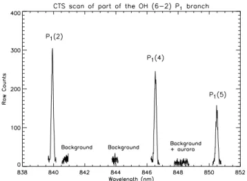
extensively studied (Greet et al., 1998). Contamination from weak auroral lines, other OH emission features, and Fraun-hoffer absorbtion lines have been identified and are allowed for or avoided in the spectra used here. Six narrow regions are scanned, corresponding to the P1(2), P1(4), and P1(5)
lines, and three background regions (see Fig. 1). Each of the OH lines are doublets, but the CTS resolution is too low to show this. The required spectral intervals were scanned every 7 minutes. Allowance is made for the scan time by linearly interpolating all intensities to a selected time between suc-cessive scans, before a rotational temperature is calculated.
The CTS has a 6 degree field of view, and was directed either to the zenith, or at a zenith distance of 70◦and geo-graphic azimuth 130◦(approximately south-east). The lat-ter was chosen to maximise the signal by looking obliquely through the atmosphere, in an azimuth opposite to usual
au-Fig. 1. Spectral scan from the CTS of part of the OH(6–2) P-branch
near λ845 nm. The spectrometer is stepped between the three lines and background regions during the course of 7 minutes.
roral displays. In this configuration a gold-coated first sur-face mirror was mounted obliquely on the laboratory roof to allow the off-zenith observations. The mirror showed no significant wavelength-dependent effects over the spectral re-gion of interest.
For derivation of temperatures, we used the method in Greet et al. (1998). The measured P–branch intensities are used to calculate the ratio of molecules in the rotational levels of the upper vibrational state. In order to determine the ra-tio of the number of molecules in the upper rotara-tional states, transition probabilities are generally required. Turnbull and Lowe (1989) have shown the absolute temperature derived from a range of published transition probabilities increases as the 1ν (vibrational quantum number difference) of the band increases. For the OH(6–2) band, Greet et al. (1998) calcu-late a range of 12 K for three sets of transition probabilities. French et al. (2000) measured the temperature-independent line ratios of the OH(6–2) band and determined the fractions of the upper rotational states that decay via each branch, en-abling rotational temperatures to be determined with an accu-racy of 2 K. The average temperatures calculated for a selec-tion of spectra using the experimentally derived ratios were within 2 K of the values obtained using the Langhoff et al. (1986) transition probabilities (French et al., 2000). For this current work we adopt the transition probabilities given by Langhoff et al. (1986). In applying this method, care must be exercised in identifying auroral and other contaminating signals, and in removing instrumental effects. Further details are given by Greet et al. (1998) and French et al. (2000). 2.2 The Fabry-Perot spectrometer
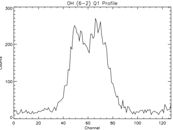
The Davis FPS is very similar to the instrument described by Jacka (1985). Slight modifications to allow OH emission observations to be made are described in Greet et al. (1994). The spectrometer uses 150 mm diameter etalon plates, is
sep-Fig. 2. Sample OH(6–2) Q1(1) profile at λ834 nm, showing the
doublet structure. Each channel is approximately 0.3 pm in width in wavelength units.
aration scanned by piezoelectric devices under servo control, and is located in a temperature stabilised cabinet. An aper-ture mask isolates the centre of the fringe pattern, which is viewed by a GaAs photomultiplier tube. Changing the plate separation scans the instrument in wavelength. Isolation of the spectral region of interest is done by interposing a 0.5 nm interference filter into the light path. In operation, the spec-trometer is typically scanned through 128 channels, where each channel is approximately 0.3 pm in width, in ∼6 sec-onds. For the OH emission either 80 or 120 such consecutive scans were added to give a single spectrum of the Q1(1)
dou-blet. A typical spectrum is shown in Fig. 2.
A periscope (0.5◦field of view) brings sky light into the
instrument. The fields of view of the FPS and CTS were coincident for the data reported here. Differences in ob-serving volumes could lead to observed temperature differ-ences from small-spatial scale atmospheric variations. As our comparison is limited to hourly and nightly averages, and as small-spatial scale effects generally are short-lived, we be-lieve time-averaged data are suitable for comparing the two instruments.
Data reduction involves, among other steps, correcting for photomultiplier dark count, correcting for the finite spectral resolution of the FPS, fitting a pair of Gaussians of identical width to the corrected spectra, and determining the temper-ature from the Gaussian width. Of specific relevance is the correction for the finite spectral resolution. The method used follows that outlined by Jacka (1985), and discussed further by Greet (1997). On each observing run, several high signal-to-noise ratio observations are obtained of a frequency sta-bilised He-Ne laser, with its emission at λ632.8 nm. The laser is assumed to have zero instrinsic line-width compared to the resolving power of the FPS; hence, the laser profile is taken as a measure of the intrinsic broadening of the instru-ment. This is termed the instrument function (see Wilksch, 1985, for a detailed discussion of this).
The instrument function will vary with wavelength, as the reflective quality of the etalon plate coatings is also a function of wavelength. Hence, we cannot directly use the λ632.8 nm laser profile to correct the λ834 nm OH spectra. The quantity that characterises the effect of the reflectivity for an FPS is the reflective finesse, F . Knowledge of the reflective finesse at the laser and OH wavelengths allows a wavelength-corrected instrument function to be found. Mea-surement of the reflective finesse, in principle straightfor-ward, is difficult in practice, and has not successfully been done for the Davis FPS at λ834 nm. Calculation of the fi-nesse can be done knowing the reflectivity of the etalon coat-ing as a function of wavelength. The manufacturer’s design specification leads to a finesse of 18 at λ834 nm. The uncer-tainty is not known, but could easily be of the order of one unit. A change in the Fλ834 finesse by one unit propagates
through to a change in the derived temperature by ∼20 K. For the reasons to be presented below, we adopt a finesse of 19.5 at λ834 nm, implying the etalon plates at this wavelength are slightly more reflective than the specifications supplied by the manufacturer. An alternative method of correcting the instrument function from the calibration to observing wave-length was used by Hays et al. (1981) for the Fabry-Perot Interferometer flown on Dynamics Explorer. Their method used detailed knowledge of the working finesse for each in-strument channel to produce the required inin-strument func-tion. We do not have such fine resolution finesse data for our instrument.
With the adopted value of finesse, the instrument function at λ834 nm can be found. In principle, this can be decon-volved from the raw data, and the resulting, narrower doublet can then be analysed. Deconvolution is normally carried out in the Fourier domain, where it becomes a simple division. We prefer to avoid the deconvolution, as noise in the data can be magnified to large levels by the division of a small number into a larger one. Hence, we fit to the data a convo-lution of the instrument function and a pair of Gaussians, as we have found this method to be the more reliable one. The temperature can then be found from the width of the fitted Gaussian. The statistical error in the fit also gives a measure of the uncertainty in the temperature determination.
Temperature comparison observations were scheduled for a two week interval in mid-June 1999. At this time FPS and CTS observations at 70◦ zenith distance, at azimuth 130◦, were obtained for each clear night. Three mostly cloud-free nights of data were obtained: Day of Year (DOY) 169, DOY 173, and DOY 174. Additional OH(6–2) observations carried out in early and late June have also been used in the temperature comparison. On DOY 159 a night of simultane-ous CTS/FPS zenith direction data were obtained as part of a study of OH intensity changes during the night hours. On DOYs 153, 175, 176, 178, and 179, the CTS only observed the zenith direction, as part of the usual program, while the FPS performed cardinal point-directed observations, which included zenith measurements once per ∼hourly cycle. For these five nights the temperature comparison was between the (zenith) CTS observations that bracket, or are adjacent
362 J. L. Innis et al.: Comparison of OH(6–2) rotational and Doppler temperatures
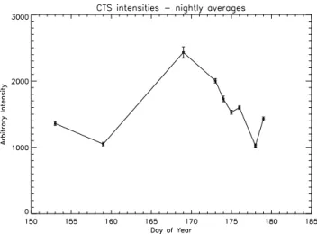
Fig. 3. Mean nightly intensities from the OH(6–2) observations
using the CTS, Davis, June 1999. One-sigma standard errors are shown.
to, the FPS zenith measurements; hence, there is one temper-ature datum every hour. For the nights of DOYs 159, 169, 173 and 174, there are temperature measurements every 6 to 7 minutes, although a small quantity of these data do not pass our acceptance criteria. A few other low quality nights from June 1999 have not been used in this comparison.
3 Results
For both instruments, summing the photon counts in the spec-tral lines gives a measure of the hydroxyl emission at the time of observation. The two intensity measures are in very good agreement, apart from a multiplicative factor due to differ-ences in the throughput. The hydroxyl emission intensity is known to be variable both during a night, and from night to night. The mean nightly intensities from the CTS are shown in Fig. 3. The greatest signal was on DOY 169.
Temperature data were determined from both CTS and FPS data, as outlined above. For the CTS data, measure-ments of temperature are obtained from each of the three pos-sible intensity ratios from the P1(2), P1(4), and P1(5) lines.
A weighted average is calculated, as described in Greet et al. (1998). The typical standard error in an individual determi-nation is 5 or 6 K. For the FPS, the observational uncertainty for each point is significantly larger, of the order of 20 to 30 K. Inspection of the distribution of the FPS measurements about the nightly mean also reveals the presence of a small number of outlying points, consisting of, at most, ∼5% of the data on any night, that do not appear to represent a real physical condition of the atmosphere. To remove these out-liers, we reject all FPS data points that are more than 80 K from the mean on a given night.
For the purposes of the comparison between the CTS and FPS temperatures, we have chosen a value of reflective fi-nesse at λ834 nm, Fλ834, of 19.5, so that the mean nightly
temperatures for one night of common observations are the
Table 1. Nightly mean temperatures with standard errors from the
CTS and FPS. The FPS data have been adjusted to bring the mean temperature from DOY 169 to be equal to that found from the CTS.
Day of Year FPS: T±s.e. (K) CTS: T±s.e. (K)
153 198±12 203±2 159 198±5 206±1 169 207±3 207±1 173 199±4 201±1 174 198±3 195±1 175 191±10 211±2 176 218±9 212±2 178 210±10 206±2 179 229±8 223±2
same. We chose for this night DOY 169, as the mean inten-sity of the OH signal was the greatest in our data set. We use this finesse value for the other nights. The adjustment made to the finesse value is not substantially different to the man-ufacturer’s specification. The present comparison between the methods is, therefore, between the temperature variations measured by each technique, rather than absolute values.
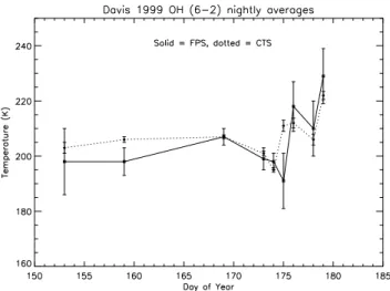
The nightly mean temperatures we obtained are given in Table 1 and are plotted in Fig. 4, along with standard errors in the means, as found from the data. The standard errors for the CTS and FPS data reflect both statistical and intrinsic variations in the data. The intrinsic atmospheric temperature variations over a night, as seen in the CTS data, are around 10 to 20 K. Statistical errors dominate in the FPS time series. We give standard errors here to indicate how well the nightly-mean FPS temperatures compare with the CTS data. The standard errors for the CTS data are given for completeness.
4 Discussion
From Table 1 and Fig. 4 it is clear that the general trend over the time series is similar for both the CTS and FPS data. The biggest difference is for DOY 175, where the FPS tem-perature is 20 K less than the CTS result. The error bars shown in Fig. 4 are one-sigma standard errors. On statisti-cal grounds, we would expect that approximately 68% of the time the measured value would be within one-standard error of the ‘true’ value. We have only a few data points to make the comparison, but excluding DOY 169, six of the eight FPS determined temperatures agree with the CTS results to within this limit, while the others agree to within two standard er-rors. (For DOY 169 the whole night FPS–CTS temperature difference was set to zero; hence, it is not included in this calculation.) As noted, the sample size is small, but the dif-ferences recorded do not appear to deviate from what would be expected, assuming the measurement errors are normally distributed with standard errors determined from the data.
The mean difference, FPS–CTS, and standard error for the eight nightly means (excluding DOY 169) is −2±3 K, which is not significantly different from zero. There may be an
in-Fig. 4. Mean nightly temperatures from the OH(6–2) observations
using the CTS (dotted line) and FPS (solid line), Davis, June 1999. One-sigma standard errors are shown. The absolute values of the FPS temperatures have been adjusted to make the nightly mean for DOY 169 equal to the CTS mean for that night. See the text.
dication of a trend in the differences over the 27 day extent of the simultaneous data, with the FPS initially being low by perhaps 5 K, and then high by the same amount, with respect to the CTS. However, the standard errors in the FPS results at the start and end of the comparison are of the order of 10 K. Additionally, we see no significant difference between the off-zenith (DOYs 169, 173 and 174) and zenith-directed data.
Hourly mean temperatures are obtainable for four days of the campaign: DOY 159, DOY 169, DOY 173, and DOY 174. These data are shown in Fig. 5. The uncertainties are neces-sarily larger, as fewer data points contribute to the hourly means than to the nightly means, but the two data sets track well. Some 70% of the FPS observations are within one stan-dard error of the corresponding CTS data point (DOY 169 is again excluded in this case). The mean difference FPS–CTS of these hourly data is −2±2 K, again not significantly dif-ferent from zero.
Temperature measurements from the FPS have a greater observational error than those obtained with the CTS. In part, this is a consequence of the high-spectral resolution of the FPS compared to the CTS, resulting in significantly reduced count rates. Each FPS profile must also have sufficient signal to enable the line shape to be well determined, rather than to give a single measure of the total count, as for the CTS. Many modern FPSs use a fixed etalon spacing and a fringe-viewing area detector to avoid the need to scan in wavelength. Such a system should provide a gain in signal-to-noise ratio per individual measurement, which may lead to a reduction in the observational error per data point. Temperature deter-minations with such systems appear more difficult than with scanning spectrometers, due to the problem of the analyses of the circular fringe pattern and the doublet nature of the OH emission, but the potential advantages could be significant.
Fig. 5. Mean hourly temperatures from the OH(6–2) observations
using the CTS (dotted line) and FPS (solid line), Davis, for four days in June 1999. Top to bottom: DOY 159; DOY 169; DOY 173; DOY 174. One-sigma standard errors are shown.
The agreement between the derived CTS and FPS temper-atures over the ∼25 K range seen during the interval of the observations in Figs. 4 and 5 give a measure of confidence that the measurements are reflecting the real state of the up-per mesosphere. We noted earlier that thermalisation of the translational degrees of freedom of the OH molecule would be expected. Our results, showing the agreement between the derived rotational and Doppler temperature changes, lend weight to this assertion.
At a detailed level, however, small differences between the two techniques may be expected. The (approximately) Gaussian height profile of the OH layer is superimposed on a small, and seasonally-variable, vertical temperature gradi-ent. Both measurements are a height-integrated, intensity-weighted, observation of the OH layer. Slightly different weighting-functions contributing to each height-integrated observation may well be expected. For the Doppler method, some slight deviation from pure Gaussian line-shapes could be present, due to contributions from emissions at the lower and upper ranges of the OH layer. However, such effects would be unlikely to be detectable with the signal-to-noise ratios we can currently obtain. Considerations of this type should, however, be noted as potential reasons why exact agreement may not occur.
The absolute temperature measured by the FPS is un-certain because the reflective finesse of the etalon plates at λ834 nm has not been well determined. For the present work, however, it is encouraging that good agreement between the two techniques can be found by the assumption of a single reflective finesse value for all the FPS data.
A method of measurement of the finesse F is described by Jacka (1985). Such measurements have been performed on our FPSs at the Antarctic stations, but not at λ834 nm for the Davis instrument. Our experience has shown the properties of the etalon coatings of the Antarctic FPSs are often stable
364 J. L. Innis et al.: Comparison of OH(6–2) rotational and Doppler temperatures over a number of years, so that a future determination of F
at λ834 nm might be useful for back-calibration of these cur-rent data. However, previous finesse measurements at other wavelengths (Murphy, 1996) have shown the difficulty of ob-taining a precise value of this quantity; the uncertainty in the result is often ±0.5 or 1 units. This propagates through the FPS temperature measurements to give a range of the order of 10 to 20 K, making impossible an absolute comparison with the CTS temperatures.
Alternatively, the effect of uncertainties in F at the ob-serving wavelength can be greatly reduced, if not completely eliminated, by using a calibration source at a very similar wavelength to determine the instrument function. For ex-ample, a single-mode, frequency stabilised laser operating, in this case, at ∼ λ834 nm would give the instrument func-tion directly at the observing wavelength, and should lead to significantly reduced absolute errors in temperature. This should provide an independent check on the adopted transi-tion probabilities and the absolute equivalence of rotatransi-tional and kinetic temperatures for the OH emission.
5 Conclusions
Wintertime upper mesosphere temperatures over Davis, Antarctica have been derived by two independent instru-ments and techniques from observations of the hydroxyl (6– 2) emissions: a Czerny-Turner spectrometer to find rotational temperatures, and a Fabry-Perot spectrometer to determine Doppler temperatures. An absolute temperature comparison cannot currently be made, due to uncertainties in the reflec-tive finesse, F , for the FPS at λ834 nm. We chose F to make the mean FPS temperature equal to the CTS temperature for the night of greatest OH emission intensity. The remaining eight nights of data show good agreement in the variations of nightly means. Hourly mean data, available from four nights of the campaign, also show good agreement between the CTS and FPS. We believe this is the first such simultaneous com-parison of these techniques of measuring upper mesosphere temperatures. Our results illustrate the essential equivalence of the techniques. Refinement of the value of the reflective finesse at λ834 nm for the FPS should allow an absolute tem-perature comparison to be made.
Acknowledgements. We thank John Everett, formerly with Aus-tralian Antarctic Division (AAD), for advice and assistance with the design and manufacture of the gold-surfaced mirror used for the CTS off-zenith observations. Andrew Fleming and Geoff Tonta (AAD Instrumentation Workshop) designed and manufactured the mirror mounting plate. Lloyd Symons (Davis 1999 electronic engi-neer) maintained and supported the instruments used in this experi-ment. Tony Morwood (Davis 1999 carpenter) co-ordinated and per-formed the installation of the gold-surfaced mirror on the laboratory roof in the middle of the Antarctic winter. John Toms (Davis 1999 mechanic) manufactured the roof mounting frame. We thank the other members of the expedition for assistance and support through the year, and Mark Conde of the University of Alaska, Fairbanks (UAF) for useful discussions. This work was supported by the AAD, the Australian Antarctic Science Advisory Committee, and
the Australian Research Council. John Innis acknowledges the hos-pitality of UAF during part of the time this paper was in preparation. We thank the referees for constructive comments.
Topical Editor D. Murtagh thanks J. Meriwether and another ref-eree for their help in evaluating this paper.
References
Armstrong, E. B., The influence of a gravity wave on the airglow hydroxyl rotational temperature at night, J. Atmos. Terr. Phys., 37, 1585–1591, 1975.
Baker, D. J. and Stair, A. T., Rocket measurements of the altitude distributions of the hydroxyl airglow, Phys. Scripta, 37, 611–622, 1988.
Bittner, M., Offermann, D., and Graef, H. H., Mesopause tempera-ture variability above a midlatitude station in Europe, J. Geophys. Res., 105, 2045–2058, 2000.
French, W. J. R., Burns, G. B., Finlayson, K., Greet, P. A., Lowe, R. P., and Williams, P. F. B., Hydroxyl (6–2) airglow emission intensity ratios for rotational temperature determination, Ann. Geophysicae, 18, 1293–1303, 2000.
Golitsyn, G. S., Semenov, A. I., Shefov, N. N., Fishkova, L. M., Lysenko, E. V., and Perov, S. P., Long-term temperature trends in the middle and upper atmosphere, Geophys. Res. Lett., 23, 1741–1744, 1996.
Greet, P. A., Innis, J., and Dyson, P. L., High-resolution Fabry-Perot observations of mesospheric OH(6–2) emissions, Geophys. Res. Lett., 21, 1153–1156, 1994.
Greet, P. A., Mesospheric observations by high-resolution Fabry-Perot spectrometers: calibrations required for climate change studies, J. Atmos. Sol. Terr. Phys., 59, 281–294, 1997.
Greet, P. A., French, W. J. R., Burns, G. B., Williams, P. F. B., Lowe, R. P., and Finlayson, K., OH(6–2) spectra and rotational temper-ature measurements at Davis, Antarctica, Ann. Geophysicae, 16, 77–89, 1998.
Hays, P. B., Killeen, T. L., and Kennedy, B. C., The Fabry-Perot interferometer on Dynamics Explorer, Space Sci. Inst., 5, 395– 416, 1981.
Hauchecorne, A., Chanin, M.-L., and Keckhut, P., Climatology and trends of the middle atmosphere temperature (33–87 km) as seen by Rayleigh lidar over the south of France, J. Geophys. Res., 96, 15297–15309, 1991.
Hernandez, G., Smith, R. W., and Conner, J. F., Neutral wind and temperature in the upper mesosphere above South Pole, Antarc-tica, Geophys. Res. Lett., 19, 53–56, 1992.
Jacka, F., Application of Fabry-Perot spectrometers of upper atmo-sphere temperatures and winds, Middle Atmoatmo-sphere Program for MAP, R. Vincent (Ed.), ch.13, 19–40, 1985.
Langhoff, S. R., Werner, H.-J., and Rosmus, P., Theoretical transi-tion probabilities for the OH Meinel system, J. Mol. Spectr., 118, 507–529, 1986.
Meriwether, J., High-latitude airglow observations of correlated short-term fluctuations in the hydroxyl Meinel 8–3 band intensity and rotational temperature, Planet. Space Sci., 23, 1211–1221, 1975.
Mulligan, F. J., Horgan, D. F., Galligan, J. G., and Griffin, E. M., Mesopause temperatures and integrated bnad brightness calculated from airglow OH emissions recorded at Maynooth (53.2◦N, 6.4◦W) during 1993, J. Atmos. Terr. Phys., 57, 1623– 1637, 1995.
Murphy, D. J., Finesse measurements of the Mawson high-resolution Fabry-Perot spectrometer, ANARE Research Notes, 95, Australian Antarctic Division, Kingston, 221–235, 1996. Myrabo, H. K., Winter-season mesopause and lower thermosphere
temperatures in the northern polar region, Planet. Space Sci., 34, 1023–1029, 1986.
Offermann, D. and Gerndt, R., Upper-mesosphere temperatures from OH∗emissions, Adv. Space Res., 10(12), 217–221, 1990. Pendleton, Jr., W. R., Espy, P. J., and Hammond, M. R.,
Evi-dence for non-local-thermodynamic-equilibrium rotation in the OH nightglow, J. Geophys. Res., 98, 11567–11579, 1993. Roble, R. G. and Dickinson, R. E., How will changes in carbon
dioxide and methane modify the mean structure of the meso-sphere and thermomeso-sphere? Geophys. Res. Lett., 16, 1441–1444, 1989.
Sahai, Y., Giers, D. H., Cogger, L. L., Fagundes, P. R., and Garbe, G. P., Solar flux and seasonal variations of the mesopause tem-peratures at 51◦N, J. Atmos. Terr. Phys., 58, 1927–1934, 1996. Scheer, J. and Reisen, E. R., Rotational temperatures for OH and
O2airglow bands measured simultaneously from El Leoncito, J.
Atmos. Terr. Phys., 52, 47–57, 1990.
Scheer, J., Reisen, E. R., Espy, J. P., Bittner, M., Graef, H.-H., Of-fermann, D., Ammosov, P. P., and Ignatyev, V. M., Large-scale structures in hydroxyl rotational temperatures during DYANA, J. Atmos. Terr. Phys., 56, 1701–1715, 1994.
Sears, F. W. and Salinger, G. L., Thermodynamics, Kinetic The-ory, and Statistical Thermodynamics, Addison-Wesley, Reading, Mass., 264–266, 1975.
She, C. Y. and Lowe, R. P., Seasonal temperature variations in the mesopause region at mid-latitude: comparison of lidar and hy-droxyl rotational temperatures using WINDII/UARS OH height profiles, J. Atmos. Sol. Terr. Phys., 60, 1573–1583, 1998. Sivjee, G. G., Airglow hydroxyl emissions, Planet. Space Sci., 40,
235–242, 1992.
Takahashi, H., Clemesha, B. R., and Sahai, Y., Nightglow OH(8– 3) band intensities and rotational temperature at 23◦S, Planet. Space Sci., 22, 1323–1329, 1974.
Takahashi, H., Clemesha, B. R., Sahai, Y., and Batista, P. P., Sea-sonal variations in the mesopause temperature observed at equa-torial (4◦S) and low (23◦N) latitude stations, Adv. Space Res., 14, 197–100, 1994.
Turnbull, D. N. and Lowe, R. P., New hydroxyl transition probabil-ities and their importance in airglow studies, Planet. Space Sci., 37, 723–738, 1989.
von Zahn, U., Fricke, K. H., Gerndt, R., and Blix, T., Mesospheric temperatures and the OH layer height as derived from ground-based lidar and OH∗ spectrometry. J. Atmos. Terr. Phys., 49, 863–868, 1987.
Wilksch, P. A., Instrument function of the Fabry-Perot spectrometer, Appl. Optics, 24, 1502–1511, 1985.