HAL Id: tel-02275552
https://tel.archives-ouvertes.fr/tel-02275552
Submitted on 31 Aug 2019HAL is a multi-disciplinary open access archive for the deposit and dissemination of sci-entific research documents, whether they are pub-lished or not. The documents may come from teaching and research institutions in France or abroad, or from public or private research centers.
L’archive ouverte pluridisciplinaire HAL, est destinée au dépôt et à la diffusion de documents scientifiques de niveau recherche, publiés ou non, émanant des établissements d’enseignement et de recherche français ou étrangers, des laboratoires publics ou privés.
tellure (Te) dans le milieu côtier : vers des scénarios de
dispersion des radionucléides de Sb et de Te en cas de
rejets accidentels de centrales nucléaires (projet
AMORAD, ANR-11-RSNR-0002)
Teba Gil-Diaz
To cite this version:
Teba Gil-Diaz. Comportement biogéochimique d’antimoine (Sb) et de tellure (Te) dans le milieu côtier : vers des scénarios de dispersion des radionucléides de Sb et de Te en cas de rejets accidentels de centrales nucléaires (projet AMORAD, ANR-11-RSNR-0002). Géochimie. Université de Bordeaux, 2019. Français. �NNT : 2019BORD0004�. �tel-02275552�
THÈSE
Présentée à
L’UNIVERSITÉ DE BORDEAUX
École Doctorale Sciences et Environnements
Par M
me
Teba GIL-DÍAZ
Pour obtenir le grade de
DOCTEUR
Label de Doctorat Européen
Spécialité : Géochimie et Écotoxicologie
Comportement biogéochimique d’antimoine (Sb) et de
tellure (Te)
dans le milieu côtier : vers des scénarios de
dispersion des radionucléides de Sb et de Te en cas de
rejets accidentels de centrales nucléaires
(PROJET AMORAD, ANR-11-RSNR-0002)
Soutenue le 11 Janvier 2019
Devant la commission d’examen formée de :
M. Nestor Etxebarria, Professeur, Université du Pays Basque, Espagne Rapporteur
M. Andrew Cundy, Professeur, Université de Southampton, UK Rapporteur
Mme. Montserrat Filella, Enseignant-chercheur, Université de Genève, Suisse Examinatrice
M. Thierry Corrège, Professeur, Université de Bordeaux Président
Mme. Elisabeth Eiche, Enseignant-chercheur, KIT, Karlsruhe, Allemagne Invitée
M. Jörg Schäfer, Professeur, Université de Bordeaux Directeur
Mme. Frédérique Eyrolle, Chercheur HDR, IRSN Cadarache Co-directrice
Coastal biogeochemical behaviour of
antimony (Sb) and tellurium (Te): an approach to Sb and Te
radionuclide dispersal scenarios in case of accidental
nuclear power plant releases
(AMORAD PROJECT, ANR-11-RSNR-0002)
Directed by:
Jörg Schäfer, Université de Bordeaux
Frédérique Eyrolle, IRSN Cadarache
dispersal scenarios in case of accidental nuclear power plant releases
Antimony (Sb) and tellurium (Te) are relatively uncommon contaminants (stable isotopes) and may form short-lived fission products (radionuclides) released into the environment during nuclear power plants accidents. Little is known about their respective biogeochemical behaviours, necessary for general contamination studies and post-accidental radiological risk assessment.
This work provides original knowledge on Sb and Te biogeochemical behaviour in highly dynamic continent-ocean transition systems: the Gironde Estuary and the Rhône River. Concentrations, spatial/temporal variations, solid/liquid partitioning (Kd), and fluxes are studied from long-term records at the watershed scale. Four estuarine sampling campaigns during contrasting hydrological conditions show higher Sb solubility and Te particle affinity in the estuary than in the upstream fluvial reaches. Historical records (1984-2017) in wild oysters from the estuary mouth do not show clear trends of past or recent contamination, but measurable bioaccumulation suggests that potential uptake of radionuclides is likely to occur. Combined adsorption experiments using isotopically-labelled (spiked) Sb and Te, and subsequent selective extractions of carrier phases from suspended particulate matter (SPM) suggest that spiked Sb and Te are more mobile and potentially bioaccessible than their environmental (inherited) equivalents. Radiotracer adsorption experiments using environmentally representative concentrations of both Gironde and Rhône systems underpin that highly soluble elements may show contrasting reactivity between inherited and spiked forms.
Radionuclide dispersion will greatly depend on (i) the geographical position of the source (Rhône) and/or the maximum turbidity zone (MTZ; Gironde fluvial-estuarine system), (ii) the succession of hydrological situations during and after the accident, and (iii) the biogeochemical reactivity and half-lives of the radionuclides. First scenarios on hypothetical dissolved radionuclide dispersion in the Gironde Estuary suggest (i) low sorption of Sb to the SPM, implying a transport of radionuclides in dissolved phase towards the coast, and (ii) high retention of Te within the MTZ, especially for accidental releases during flood conditions, linking the fate of radioactive Te to long estuarine SPM residence times (1-2 years). Potential upstream migration of Te radionuclides in the MTZ towards the city of Bordeaux during the following summer season and Te decay into radioactive iodine warrants further evaluation of the associated potential radiotoxicity.
Keywords: antimony, tellurium, Gironde Estuary, solid/liquid partitioning (Kd), selective extractions
Comportement biogéochimique d’antimoine (Sb) et de tellure (Te) dans le milieu côtier : vers des scénarios de dispersion des radionucléides de Sb et de Te en cas de rejets accidentels de centrales nucléaires
Antimoine (Sb) et tellure (Te), sont des contaminants peu étudiés (isotopes stables) et leurs radionucléides artificiels peuvent être rejetés dans le milieu aquatique lors des accidents nucléaires. La connaissance de leurs comportements biogéochimiques respectifs est nécessaire à l'évaluation du risque radiologique post-accidentel.
Ce travail présente des données originales sur le comportement biogéochimique de Sb et de Te dans les systèmes de transition continent-océan, tels que l'estuaire de la Gironde et la rivière du Rhône. Un suivi de 14 ans et des campagnes océanographiques dans le bassin versant de l’estuaire de la Gironde ont permis d’identifier des concentrations, des flux, et des réactivités (variabilités spatio-temporelles et distribution solide/liquide) plus élevés pour Sb que pour Te, mettant en évidence un comportement additif pour Sb et de soustraction pour Te le long des gradients de salinité et de turbidité estuariennes. Des expériences couplant l’adsorption d’isotopes marqués sur des matières en suspension (MES) et des extractions sélectives des phases porteuses, suggèrent que les formes apportées deSb et de Te sont plus mobiles et potentiellement plus biodisponibles que leurs équivalents naturels. De plus, l’observation de la bioaccumulation non-négligeable de Sb et de Te naturels dans les huîtres sauvages à l’embouchure de l’estuaire permet d’envisager une absorption potentielle de leurs homologues radioactifs.
Ainsi, le développement de scenarios de dispersion de radionucléides rejetés dans les zones de transition dépendra (i) de la position géographique de la source (Rhône) et/ou de la zone de turbidité maximale (ZTM; système fluvio-estuarien de Gironde), (ii) de la situation hydrologique pendant et post accident, ainsi que (iii) de la réactivité biogéochimique et des temps de demi-vies des radionucléides. Les premiers scénarios de dispersion de radionucléides
dans l'estuaire de la Gironde suggèrent (i) un transport préférentiel de Sb dissousvers la zone côtière, et (ii) une forte
rétention de Te radioactif dans la ZTM si la dernière est présente en aval du site d’accident, impliquant le risque de migration saisonnière de la radioactivité vers la ville de Bordeaux pendant l’étiage suivant. Ainsi, la dynamique intra estuarienne (marée, débit et migration de la ZTM) sera le facteur prédominant dans le devenir de Te radioactif, depuis son rejet jusqu’à sa désintégration complète en iode radioactif. L’ensemble de ce travail met en évidence la nécessité d’une évaluation plus approfondie de la radiotoxicité potentielle de Sb et Te lors de leurs rejets en milieu aquatique.
This work is a scientific contribution to the French National Project AMORAD
(ANR-11-RSNR-0002) from the National Research Agency, allocated in the
framework programme “Investments for the Future”.
Partial funding by the ANR Programme TWINRIVERS (ANR-11-IS56-0003) and the
FEDER Aquitaine-1999-Z0061 are greatly acknowledged. Support from “l’Agence
de l’Eau Adour-Garonne” and the European Project SCHEMA (EU FP7-OCEAN
2013.2-Grant Agreement 614002) are also acknowledged.
This work has benefited from environmental samples (i) from the RNO/ROCCH
oyster sample bank (Ifremer Centre Atlantique, Nantes), and (ii) from the IRSN
mussel sample bank and SORA Station (Arles).
J’ai le grand plaisir de faire un récapitulatif de toutes les personnes qui ont eu un rôle significatif, voire très important, au cours de ma thèse pour arriver aujourd’hui à avoir ce travail de trois ans de vie. Personnellement, c’est la meilleure trace écrite que j’aurai dans l’avenir pour déclencher ma joie et des larmes de nostalgie à chaque fois que j’y reviendrai pour me rappeler de toutes les belles expériences vécues et les personnes inoubliables de ces dernières années… car si on avance dans la science c’est parce qu’on n’est pas seul.
Tout d’abord, je voudrais remercier les membres de mon jury de thèse d’avoir accepté de corriger et d’évaluer ce travail. I am very grateful to Nestor ETXEBARRIA, Andrew CUNDY, Montserrat FILELLA and Thierry CORRÈGE for their availability and interest in reviewing this work.
Un grand merci à mes directeurs de thèse Jörg SCHÄFER et Frédérique EYROLLE-BOYER pour m’avoir donné ce sujet de thèse et le travail associé, qui avait déjà commencé pendant mon stage de master M2. Depuis ce temps et grâce à eux, j’ai eu énormément d’opportunités pour profiter de leur expertise en géochimie et radioactivité environnementale et beaucoup de plaisir à partager mes travaux sous leur direction dans plusieurs conférences et réunions du projet AMORAD. Je vous remercie d’avoir toujours cru en mes compétences, d’avoir partagé votre joie scientifique à chaque découverte le long du chemin et d’avoir toujours soutenu l’objectif de cette thèse malgré les adversités. Merci Jörg pour la liberté et le soutien scientifique, toujours présents.
Je voudrais remercier Alexandra COYNEL pour tous ses bonnes remarques et corrections dans les publications qu’on a en commun et surtout de m’avoir donné l’opportunité de commencer ma carrière dans le monde de l’enseignement pendant ma troisième année de thèse à plusieurs niveaux de l’éducation universitaire (licence et master). Surtout, merci de m’avoir transmis qu’en science et dans l’enseignement il faut toujours viser à bien faire les choses, et de m’avoir appris dès le début qu’une thèse « n’est pas un sprint mais un marathon » … merci d’avoir veillé au soutien financier des trois derniers bornes.
Je remercie Gérard BLANC pour sa bonne humeur et les sourires de chaque jour. On n’a pas eu l’opportunité de travailler beaucoup ensemble mais je vous remercie de m’avoir accepté et bien accueilli dans l’équipe pendant tout ce temps.
Merci beaucoup Fred FAURE-POUGNET pour un milliard de choses, entre lesquelles je garde précieusement : ta force en esprit (dans le personnel et professionnel), pour tous ces années au bureau, d’avoir partagé avec moi ta connaissance sur la dynamique de l’estuaire et le comportement du Cd et des butyl-Sn, de m’avoir permis d’échantillonner avec toi pendant MGTS 3, de m’avoir laissé analyser tous tes échantillons de MGTS en cherchant les comportements environnementaux de Sn, de
d’être là jusqu’à la fin…
Merci beaucoup Mélina ABDOU aussi pour plein de choses : d’être là pour m’aider à ne rien oublier et préparer les colis d’échantillons à chaque fois que je partais en stage en Allemagne, d’avoir partagé avec moi 5 campagnes océanographiques dans plusieurs endroits européens (avec la préparation du mathos et tout l’expertise inclus), d’avoir vécu les adversités environnementales implicites dans chaque mission (p.e. l’attaque d’une centaine d’insectes volants sur le bateau à 4h du matin !), d’avoir partagé aussi tes découvertes sur le comportement du Pt en milieu aquatique, d’avoir assisté à plus de
5 conférences ensemble, sans manquer >105 sourires et rigolades au cours de tous ces moments !!
Ne t’inquiètes pas Antoine LERAT, j’ai aussi beaucoup à te remercier ! Pour tous ces années de partage de bureau aussi, nous permettant d’avoir plusieurs discussions sur tous les sujets (sur la vie du labo, nos travaux, l’enseignement), toujours « scientifiquement pertinentes » bien sûr ! Merci d’avoir partagé avec moi tes joies et challenges avec le Gd, toujours enrichissants ! de m’avoir laissé afficher mes posters sur ta partie du mur :P et d’avoir veillé sur moi pendant les dernières mois de rédaction.
Je voudrais remercier Clément PERETO, pour son aide précieuse avec le traitement de données ICP-OES, les discussions scientifiques de bureau sur les transferts des métaux vers le biote, la dernière sortie Decaz en Août 2018, et les moments de détente au Carpe. A Mathilde MYKOLAZYCK et Ane REMENTERIA pour toutes leurs expertises en manipulation d’huîtres sauvages et l’assimilation en Cd et Ag. A Guia MORELLI pour son soutien moral et le travail sur les carottes estuariennes. A Stéphane AUDRY pour son aide indirect grâce à sa thèse au sein de l’équipe TGM sur les extractions sélectives en métaux classiques ainsi que de Sb et As.
A Lionel DUTRUCH et Cécile BOSSY, sans lesquels je n’aurai jamais su traiter les échantillons (attaques, acidifications), doser tous les éléments que j’ai étudié, utiliser tous les techniques analytiques (dilution gazeuse, iCAP), faire les bons calcouls de traitement de données, commander les bons matériaux de labo, faire une grande partie des missions Decaz, etc. Merci beaucoup d’avoir toujours répondu à absolument toutes mes questions de labo, en personne et par email, toujours avec des réponses « techniquement correctes » !
Merci Hervé DERRIENNIC, Marie BILLA et Eric MANEUX qui ont fait partie de ma vie quotidienne de labo. Je remercie aussi à mes stagiaires au cours des années : Linda, Thomas, Ruoyu, Khalil, Virginia, JB et Madhushri. Travailler avec vous a été souvent une expérience très stimulante, merci de votre aide et enthousiasme inépuisable pour le travail de labo.
year of PhD in Karlsruhe (Germany). Thank you Eli EICHE for integrating me so naturally in the team and for your resourcefulness in equipment and Se contacts. I will always recall your constant impulse, good advice and optimism despite the « challenging » water and sediment samples that I brought to you. After all, Se was indeed an « analytical chemist’s nightmare » but we managed to advance and characterise its behaviour and concentrations in some of my sample matrices. I thank Markus LENZ for accepting the challenge to double-check Se and Te concentrations in the freshwater and some sediment-digested samples with his new triple-quad ICP-MS in Basel (Switzerland). I also thank very much Gesine PREUΒ and Claudia MÖΒNER, for spending some time sharing their enthusiasm, working precision and knowledge on GF-AAS and ICP-MS at KIT. Thanks to Beate OETZEL for her help in milling and preparing the samples for ED-XRF and XRD measurements. Many thanks to Utz KRAMAR and Andreas HOLBACH for their guidance in ED-XRF world as well as Kirsten DRÜPPEL for her help in the XRD interpretations. Many thanks to Andrea FRIEDRICH for all her paperwork assistance, Gerhard OTT for connecting my French PC to the network and printers in the lab and to Ralf WACHTER for fixing every machine (microwave, stove, water tank) that gave problems. I also thank Alexandra NOTHSTEIN and Helena BANNING for their help in HG method and performance. My office and lunch-mates, Andrew THOMAS and Flavia DIGIACOMO, thanks for making me discover the Mensa and the AKK. From the personal point of view, I owe a big thanks to Sandra KLINGLER, Christine BRAUN, Eugen BLUM and the BURY’s family for being so kind and helpful, for showing me new places in the region and for making my stay in Germany possible, enjoyable and unforgettable; Vielen Dank.
I also have a special thanks to Frank HEBERLING for giving me a second chance to come back to
Karlsruhe during my last year of PhD to measure sorption kinetics of radioactive elements (113Sn and
75Se) at the INE KIT in the Northern Campus. I’m very grateful for this opportunity and for all the advices
on practical and theoretical knowledge about radioactive handling and decay. Thank you for always being positive, patient and willing to help. I would also like to thank Bernd BUMMEL and Andreas BAUER for all their help allowing me to getting started (and the bike!), as well as Melanie BÖTTLE and Markus FUSS for the gamma spectroscopy measurements and explanations on HPGe detectors. I
greatly acknowledge Christian MARQUARDT for arranging all the paperwork for the 113Sn and 75Se stock
solutions, Tanja KISELY for supplying the clothes and all labware every time I asked for it, David FELLHAUER for all the advices on good practices in the controlled-area, and a special thanks to Gerhard CHRISTILL for being patient when I had to sample near the closing time and allowing me to take pictures of my experimental setup. Many thanks to Frank BECKER for his help with radioactive decay chains and understanding of fission yields, and to all the team from INE (including all the PhD and master students: Fabian, Jurij, Nese, Nicoletta, Tims, ...) for their smiling Gütten Morgen and nice meals together every day.
échantillons de MES du Rhône, toujours présent par email pour répondre à mes questions sur le Rhône et pour résoudre les défis de la poste concernant la réception des colis à Bordeaux. Je remercie également Sabine CHARMASSON de l’IRSN - Centre IFREMER de la Méditerranée pour l’envoi des échantillons de moules de la banque biologique de la Méditerranée, et surtout pour son soutien et bienveillance tout le long du projet AMORAD en tant que responsable scientifique de l’axe de recherche Marin.
Je remercie énormément Nicolas BRIANT, Teddy SIREAU et Jöel KNOERY du Centre Atlantique IFREMER d’avoir partagé avec nous les échantillons d’huîtres du suivi RNO/ROCCH. Merci beaucoup de m’avoir accueilli très chaleureusement pendant mon séjour de <24h à Nantes, de votre bienveillance pendant les minéralisations et merci pour les corrections apportées au travail final avec les résultats de Te.
Je tiens à remercier toutes les personnes que j’ai pu rencontrer et avec lesquels j’ai eu la chance de partager des journées enrichissantes pendant les missions terrain. Je pense particulièrement aux personnes du Projet SCHeMA (Mary-Lou, Abra, Silvia, Lukas, Marianna, Maria, Nadia, Miguel, Michaela, Francesco) et à celles du PiE à Plentzia (Ionan, Manu, Urtzi, Tifanie, …).
I thank the MER family (Fouzia, Pauline, Kiyo, Marina, Ankje, Tamer, Niko, Whollie) for always being there, on the other side of the screen during our skype group calls, ready to share and listen all our worldwide adventures no matter how early in the morning your local time slots had to be. I also thank my friends and flat mates (Arielle IKI, Chris BOEIJE, Alberto ADÁN, Luca PERUZZO, Irene TONELATO, Daniela ROSSO, Tamara MAURY and Corentin DETRE) for all the trips, games, movies, dinners and birthdays, every moment duly flavoured with good cider and many laughs.
Y ya que se están convirtiendo en unos agradecimientos internacionales no podía terminar de otra manera. A las chicas de CCMar (Marta, Nadia, Lourdes, Jesenia), porque a pesar de las vueltas que da la vida, el tiempo no pasa para nosotras. A Sele y Óscar, por apuntar en el calendario todas las fechas en las que vuelvo a casa. A Aída, Fernando y mis padres, porque sin vuestro apoyo y confianza no habría llegado hasta aquí.
“The misconceptions about the effects of radiation and the psychological effect
of not understanding the risks are far greater than the radiation risk itself”
Prof. Gerry Thomas (Imperial College)
GENERAL INTRODUCTION
I. CONTEXT ... 1
1. WORLDWIDE ENERGY DEMAND: THE REASON FOR NUCLEAR ENERGY PRODUCTION ... 1
2. EUROPEAN CONCERN ON THE NUCLEAR ENERGY INDUSTRY: A FOCUS ON RADIOECOLOGY ... 4
II. THE RESEARCH QUESTION ... 6
1. NUCLEAR ENERGY IN FRANCE: CURRENT STATUS AND FUTURE PLANS... 6
2. IMPROVED FRENCH APPROACH TO POST-ACCIDENTAL MANAGEMENT:THE AMORADPROJECT ... 7
III. THESIS OBJECTIVES AND CHAPTER DISTRIBUTION ... 12
CHAPTER 1: SCIENTIFIC CONTEXT
I. INTRODUCTION ... 16II. ISOTOPES AND RADIOACTIVITY ... 17
1. ATOMIC DEFINITIONS, ELEMENTAL ABUNDANCE AND ISOTOPE STABILITY ... 17
2. DECAY MODES ... 20
3. ENERGY AND RADIOACTIVITY UNITS ... 22
4. EXPOSURE TO RADIATION AND BIOLOGICAL IMPLICATIONS ... 22
III. RADIONUCLIDES FROM NUCLEAR POWER PLANTS (NPP)... 26
1. NUCLEAR FISSION PRINCIPLES AND NPP ELECTRICITY PRODUCTION ... 26
2. CAUSES OF PAST NPP ACCIDENTAL EVENTS ... 28
3. EXAMPLES OF NPP INCIDENTS IN FRANCE ... 30
4. ENVIRONMENTAL LESSONS FROM PAST NPP ACCIDENTAL EVENTS: CASE OF CS IN AQUATIC SYSTEMS ... 31
IV. RADIOACTIVE AND STABLE ISOTOPES OF ANTIMONY AND TELLURIUM ... 34
1. RADIOACTIVE ANTIMONY (SB) AND TELLURIUM (TE) ... 34
1.1. Radionuclides of Sb and Te in NPPs ... 34
1.2. Knowledge on Sb and Te radionuclide environmental releases ... 35
Radioactive Sb ... 35
Radioactive Te ... 37
1.3. Antimony and tellurium radioactive decay chains ... 39
2. STABLE ANTIMONY (SB) AND TELLURIUM (TE) ... 44
2.1. Sources, applications, chemical properties, concentrations and toxicity of stable Sb ... 45
2.1.1. Anthropogenic sources and applications ... 45
2.1.2. Environmental speciation and redox dynamics ... 47
2.1.3. Environmental concentrations and biogeochemical behaviour ... 60
2.1.4. Biological uptake and toxicity... 71
2.2. Sources, applications, chemical properties, concentrations and toxicity of stable Te ... 72
2.2.1. Anthropogenic sources and applications ... 72
2.2.2. Environmental speciation and redox dynamics ... 76
2.2.3. Environmental concentrations and biogeochemical behaviour ... 78
2.2.4. Biological uptake and toxicity... 80
CHAPTER 2: MATERIALS AND METHODS
I. INTRODUCTION ... 83
II. AREAS OF STUDY AND SAMPLING SITES ... 84
1. AREAS OF STUDY ... 84
1.1. The Lot-Garonne-Gironde fluvial estuarine system ... 84
1.1.1. The Lot River watershed ... 85
1.1.2. The Gironde Estuary ... 86
1.1.3. Nuclear power plants ... 88
1.2. The Rhône River ... 90
1.2.1. Nuclear power plants ... 91
2. ENVIRONMENTAL MONITORING: FLUVIAL AND ESTUARINE SAMPLING SITES... 92
3. SPORADIC SAMPLING: COLLECTION OF SPECIFIC ENVIRONMENTAL MATRICES ... 94
III. SAMPLING STRATEGIES ... 96
1. LABWARE PRE-CONDITIONING, SAMPLED PHASES AND FIELD WORK APPROACH ... 96
2. RIVER DISCHARGES,SPM CONCENTRATIONS AND PHYSICAL-CHEMICAL PARAMETERS ... 100
3. COLLECTION OF WATER AND SPM SAMPLES ... 100
4. COLLECTION OF BIOLOGICAL SAMPLES ... 101
IV. EXPERIMENTAL DESIGNS ... 102
1. ISOTOPICALLY-LABELLED KINETIC EXPERIMENTS ... 102
1.1. Adsorption kinetics and isotherms of stable 125Te and 77Se ... 102
1.2. Adsorption/desorption kinetics of 75Se and 113Sn radiotracers ... 104
2. ADSORPTION OF ISOTOPICALLY-LABELLED SPIKES FOR PARALLEL SELECTIVE EXTRACTIONS ... 107
V. SAMPLE PRE-TREATMENT ... 108
1. SAMPLE DRYING ... 108
1.1. Sediments ... 108
1.2. Biological materials ... 108
2. BULK SEDIMENT MINERALOGY PREPARATIONS ... 109
3. DIGESTIONS AND SELECTIVE EXTRACTIONS OF SEDIMENTS ... 110
4. DIGESTIONS OF BIOLOGICAL MATRICES ... 114
VI. ANALYTICAL METHODS ... 117
1. BULK MINERALOGY ... 117
1.1. Principle of X-Ray Powder Diffraction (XRD) analysis ... 117
2. ANALYSES OF STABLE TRACE ELEMENT CONCENTRATIONS ... 118
2.1. Principle of mass spectrometry (ICP-MS) ... 118
2.2. Single vs triple quadrupole ICP-MS performance ... 120
2.3. Quantification methods ... 124
2.3.1. External calibration ... 124
2.3.2. Isotopic dilution (ID) ... 126
2.4. Analytical quality control ... 127
2.5. Applied analyses for Sb, Te and Se quantification ... 128
3. ANALYSES OF RADIONUCLIDE ACTIVITIES ... 130
3.1. Principle of gamma-ray spectroscopy ... 130
3.2. High Purity Germanium detectors ... 131
1. STATISTICAL APPROACH ... 134
1.1. Temporal series: trends and seasonal components ... 134
1.2. Dissolved and particulate annual fluxes ... 135
2. TRACE ELEMENT SOLID/LIQUID EQUILIBRIUMS ... 138
2.1. Sorption isotherms ... 138
2.2. Solid/liquid partition coefficient (Kd) ... 140
3. ENRICHMENT FACTORS ... 142
3.1. Geoaccumulation index (I’geo) ... 142
3.2. Bioaccumulation factor (BAF) ... 143
VIII. CONCLUSION ... 145
CHAPTER 3: Biogeochemical behaviour of antimony in the
Lot-Garonne-Gironde fluvial estuarine system
I. INTRODUCTION ... 1461. BIOGEOCHEMICAL BEHAVIOUR OF ANTIMONY IN THE FRESHWATER DOMAIN OF THE GIRONDE ESTUARY. . 148
2. BIOGEOCHEMICAL BEHAVIOUR OF ANTIMONY IN THE SALINITY AND TURBIDITY GRADIENT OF THE GIRONDE ESTUARY. ... 182
II. CONCLUSION ... 208
CHAPTER 4: Particulate carrier phases of Sb, a fractionation approach
I. INTRODUCTION ... 2101. SELECTIVE EXTRACTION METHODS ... 211
1.1. Origin and evolution of most known selective extraction methods ... 211
1.2. Important known modes of action of reducible (Fe/Mn oxide) fraction methods ... 218
1.3. Parallel selective extractions and total digestions: overview of bulk sediment carrier phases ... 222
2. PARALLEL SELECTIVE EXTRACTIONS ON PARTICULATE ANTIMONY ... 225
II. CONCLUSION ... 245
CHAPTER 5: Biogeochemical behaviour of tellurium in the
Lot-Garonne-Gironde fluvial estuarine system
I. INTRODUCTION ... 2471. BIOGEOCHEMICAL BEHAVIOUR OF TELLURIUM IN THE FRESHWATER DOMAIN OF THE GIRONDE WATERSHED…. ... 248
2. BIOGEOCHEMICAL BEHAVIOUR OF TELLURIUM IN THE SALINITY AND TURBIDITY GRADIENT OF THE GIRONDE ESTUARY ... 277
estuarine systems – a comparative approach between the Gironde Estuary and
the Rhône River
I. INTRODUCTION ... 302
1. REACTIVITY OF TIN AND SELENIUM RADIONUCLIDES WITH PARTICLES FROM THE GIRONDE AND RHÔNE FLUVIAL -ESTUARINE SYSTEMS IN SIMULATED CONTRASTING -ESTUARINE CONDITIONS ... 303
2. TRANSFER OF SN AND SE TO WILD LIVING BIVALVES ... 322
2.1. Bioaccumulation in wild oysters and mussels ... 322
2.2. Organotropism in wild oysters from the Gironde Estuary ... 325
II. CONCLUSION ... 327
DISCUSSION
I. FUNDAMENTAL PARAMETERS FOR RADIONUCLIDE DISPERSION SCENARIOS ... 3281. INHERITED VS SPIKED SOLID/LIQUID PARTITIONING (KD) ... 328
2. TEMPORAL COUPLING BETWEEN RADIONUCLIDE DECAY TIME SCALES AND HYDROLOGICAL PROCESSES ... 329
II. MULTI-ELEMENT RADIONUCLIDE DISPERSION SCENARIOS IN THE GIRONDE ESTUARY... 333
GENERAL CONCLUSIONS AND PERSPECTIVES
I. GENERAL CONCLUSIONS... 344 II. PERSPECTIVES ... 350RESUME ETENDU
………. 355REFERENCES
………. 364SCIENTIFIC PRODUCTION
………. 393GENERAL INTRODUCTION
Figure 1. Worldwide largest electricity end uses (Australia, Austria, Canada, Czech Republic, Finland, France, Germany, Greece, Ireland, Italy, Japan, Korea, New Zealand, the Netherlands, Spain, Sweden, Switzerland, the United Kingdom and the United States). Other industries include agriculture, mining and construction. Passenger
cars include cars, sport utility vehicles and personal trucks (IEA 2017). ... 1
Figure 2. Worldwide statistics on: (a) electricity generation by fuel type (1971-2015), (b) source shares of electricity generation (1973 and 2015 as examples), (c) nuclear electricity production by region (1971-2015), and (d) outlook to 2040’s total primary energy supply by fuel type and socio-economic predicted scenario. Countries are classified according to their attachment to the Organisation for Economic Co-operation and Development (OECD; IEA 2017)... 2
Figure 3. Spatio-temporal phases after a nuclear incident/accident. (Modified from IRSN 2014)... 5
Figure 4. French Nuclear Power Plant (NPP) network. Range of operating starting year for all reactors per NPP (brackets). Legend shows reactor differences by energy generating capacity (Megawatts electric, MWe) and reactor characteristics: single wall lined reactor with steel sealing skin (CP0 and CPY, red), double concrete reinforcement for accident prevention (P4 and P'4, yellow), compact steam generator with higher reliance on computer software (N4, blue), and new generation reactor under construction (EPR, pink). (Modified from ANS 2016). ... 6
Figure 5. Post-accidental approach to evaluating the radiological risk and dosimetry consequences of a nuclear accident in the environment (left) together with the role of the AMORAD project in such approach (right). The central question of the AMORAD project (in quotes) and the two main research domains including (i) environmental interfaces (MARIN, CONTI, ATMO), and (ii) consequences on the biosphere (ECOTOX), are also shown ... 10
CHAPTER 1: SCIENTIFIC CONTEXT
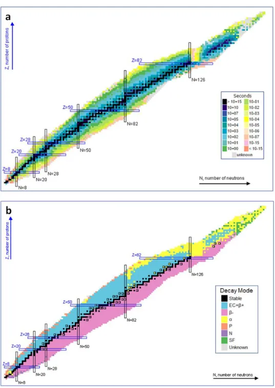
Figure 6. Binding energy as a function of mass number, showing the three main regions determining nuclear stability, indicating which elements are used in nuclear fission and which in nuclear fusion processes. (Adapted from UiO Chemical Institute). ... 18Figure 7. Segré Diagram Chart of radionuclides. (Sonzogni et al. 2013). ... 19
Figure 8. Main environmental pathways of human radiation exposure (IAEA 1991). ... 25
Figure 9. Smoothed probability distribution of fission products produced from 233U, 235U and 239Pu thermal neutron induced fission (Adapted from Seaborg and Loveland 1990). ... 26
Figure 10. General scheme of a Pressurised-Water Reactor (PWR) in a NPP (Miller 2012) ... 27
Figure 11. International Nuclear and Radiological Event Scale, INES (IAEA 2017). ... 28
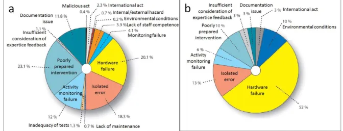
Figure 12. Summary of breakdown declared incidents in French NPPs in the year 2005 concerning (a) safety and (b) environmental incidents, classified according to main cause. (ASN Annual Report). ... 31
Figure 13. Decay chains of Sb and Te radionuclides. Information on corresponding half-lives (below each isotope AX), decay modes (electron capture-EC, beta decay-β-, isomeric transitions-IT), decay direction (red arrows), decay probability (from 0 to 1) and independent fission yields (FY) for 235U/239Pu fuels (above each isotope AX) are given. Metastable nuclides (in orange) and respective half-lives are also shown when appropriate, not specifying their probability of being formed. Empty arrows on the right (blue) denote the decay lines containing the most followed-up Sb and Te radionuclides after NPP accidental events. (The above decay chains have been assembled using available data from Element Collection Inc., and Sonzogni 2013). ... 43
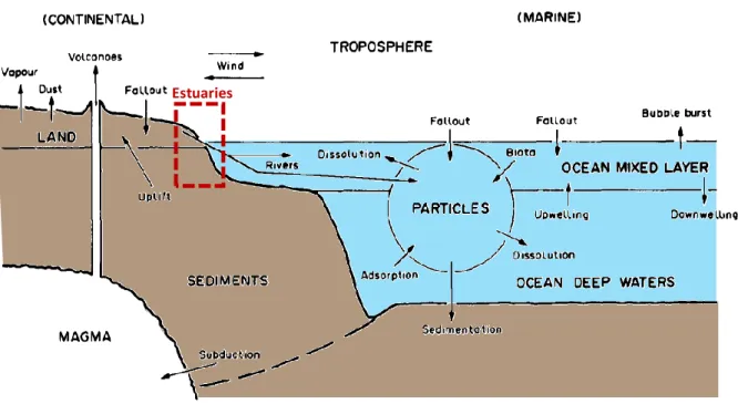
Figure 14. Schematic example of environmental compartments considered in geochemical cycling models. Global biogeochemical cycles of trace elements consider several main reservoirs (in capital letters) interacting by fluxes (arrows). Estuaries are highlighted in a red box (Austin and Millward 1967). ... 44
Figure 15. Atmospheric Sb trends by sectors (Tian et al. 2014) ... 46
Figure 16. Worldwide Sb production between 1900 and 2015 (Mlynarski 1998). ... 46
of total dissolved Sb of 10 mol L at 25ºC, showing with shaded areas the exceeding solubility of Sb relevant solids (Krupka and Serne 2002). ... 50 Figure 19. Separation of metal ions and metalloid ions (As(III) and Sb(III)) into Pearson’s modified classification: class A, borderline and class B. This classification is based on indices where χm is the metal-ion electronegativity
(Pauling’s units), r is the ionic radius (crystal IR in angstrom units) and Z its formal charge. Specified oxidation states of Pb, As, Sb and Sn imply that simple cations do not exist even in acidic aqueous solutions. Elements of interest for this work have been highlighted (red). Tellurium (IV) has been added to the original image. (Modified from Nieboer and Richardson 1980). ... 52 Figure 20. Antimony dissolved (µg L-1, 0.45 µm filtered, N = 807; a) and particulate (mg kg-1, <63 µm grain-size,
N = 848; b) concentrations in European streams sampled between 1998 and 2001 and analyzed between 1999 and 2003 (Salminen et al. 2005). ... 61 Figure 21. Worldwide Sb dissolved concentrations (ng L-1) analysed since 1980’s to 2000 for several rivers,
groundwater and tap water samples (data compilation from Filella et al. 2002a) distributed by countries: Canada (CA), United States (US), Amazon River (Amazon), United Kingdom (UK), Sweden (SE), Netherlands (NL), Germany (DE), France (FR), Portugal (PT), Spain (ES), Poland (PO), Japan (JP) and other Asian countries (Taiwan, Indonesia, etc.). Published worldwide average freshwater concentration ranges (shaded in grey area). Noteworthy the change in scale to distinguish concentrations from highly polluted sites (a) and natural concentrations (b). Most commonly observed dissolved Sb estuarine behaviours along the salinity gradient (c) are also shown for the Tamar Estuary (UK; van den Berg et al. 1991), the Tama Estuary (JP; Byrd 1990), the Scheldt Estuary (NL; van der Sloot et al. 1985), the Tagus Estuary (PT; Andreae et al. 1983) and the St. Mary’s Estuary (US; Byrd 1990). Surface seawater endmember (sw; Filella et al. 2002a) is also depicted at a random salinity of S = 40. ... 62 Figure 22: Surface seawater total dissolved Sb concentrations published between 1960 and 2000. Average and standard deviation deduced for the last 15 years is also shown (Filella et al. 2002a). ... 70 Figure 23. Worldwide Te production (t y-1) between 1900 and 2015 (Mlynarski 1998). ... 73
Figure 24. Periodic Table highlighting assigned Technology Critical Elements (red). Tellurium is denoted by a black square. (Modified from Cobelo-García et al. 2015). ... 74 Figure 25. Common environmental chemical species of Te (compilation from Belzile and Chen 2015, Wang 2011 and references therein. Humble Te speciation in aqueous media adapted from Brookins 1988). ... 77 Figure 26. Eh-pH (Pourbaix) diagram of aqueous speciation of Te. Modelling conditions include concentrations of total dissolved Te of 10-6 mol L-1 at 25ºC (Lombi and Holm 2010). ... 78
Figure 27. Environmental concentrations of dissolved Te in (a) European streams sampled between 1998 and 2001 and analysed between 1999 and 2003 (µg L-1, 0.45 µm filtered, N = 807; Salminen et al. 2005), and (b) in
surface seawater between 1980 and 2010 (ng L-1), with (c) a zoom in box for data <1 ng L-1 before 1990 (Modified
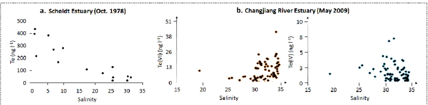
from Filella 2013). ... 79 Figure 28. Dissolved Te reactivity along salinity gradients of the Scheldt Estuary (total Te; van der Sloot et al. 1985) and the Changjiang River Estuary (speciation; modified from Wu et al. 2014). ... 80
CHAPTER 2: MATERIALS AND METHODS
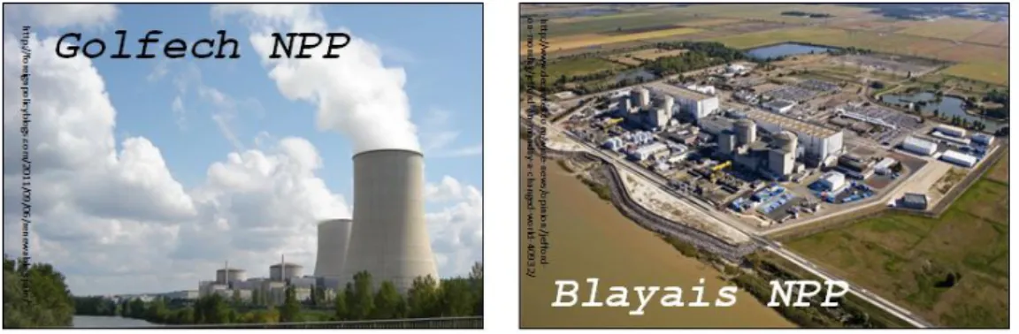
Figure 29. The Lot-Garonne-Gironde fluvial estuarine system. Rock composition along the watershed is denoted by the colour code legend (Adapted from BRGM 2014). Information on the location of the upstream historical industrial site (industrial icon), the city of Bordeaux (black circle) constituting the kilometric point zero, the assigned estuarine kilometric points (KP) and the two nuclear power plants in the area (Blayais and Golfech) are also shown. ... 84 Figure 30. Water discharge trend (1959-2017) in the Garonne and Dordogne Rivers. (Adapted from DIREN) . 85 Figure 31. Natural lithology and presence of anthropogenic tailings in the Riou Mort River watershed. Location of the historical industrial activities in Decazeville area is also presented (adapted from Coynel et al. 2007a). .. 86 Figure 32. Vertical turbidity gradient of the maximum turbidity zone (MTZ) in the water column of the Gironde Estuary. SPM: suspended particulate matter. (Modified from Audry et al. 2006, after Abril et al. 1999 and Robert et al. 2004). ... 87 Figure 33. Golfech and Blayais NPPs in the Garonne-Gironde fluvial estuarine system. ... 88 Figure 34. Sources and associated events causing potential flooding of the Blayais NPP. Failure of NPP structures (red crosses) and water overflowing into the NPP (arrows) are depicted (IRSN View-point Report 2007). ... 89
facilities (power plants and fuel reprocessing plant) are shown. Rock composition along the watershed is denoted by the colour code legend (Adapted from Ollivier et al. 2010). ... 90 Figure 36. Current NPPs in the Rhône River watershed. ... 91 Figure 37. Diagram of a steam generator of a PWR. The effect of tube plate clogging is also represented. (Adapted from IRSN View-point Report 2007 and Yang et al. 2017). ... 92 Figure 38. Sampling sites in the Lot-Garonne-Gironde fluvial estuarine system. Sampling sites are shown for the long-term monitoring programmes in the (i) upstream Lot-Garonne watershed (white squares), and (ii) estuary mouth (star), as well as for historical sediment records from hydroelectric reservoir lakes in Cajarc and Marcenac (black rectangles), sporadic samplings in Portets and Arcachon (black triangles) and from oceanographic campaigns (white and black crosses). ... 93 Figure 39. Size distribution of particles and colloidal compounds in aquatic environmental samples. (Adapted from Buffle and Van Leeuwen 1992). ... 97 Figure 40. Diagram of sampling sites and sample collection in the Lot-Garonne-Gironde fluvial estuarine system. ... 99 Figure 41. Materials for measuring SPM concentrations and physical-chemical parameters. (a) Filtration unit and pump, (b) dried filters showing contrasting SPM loads from different monitoring sites, and (c) in situ quantification of physical chemical parameters. ... 100 Figure 42. Example of (a) fluvial water and SPM collection, (b) water collection in the Gironde Estuary and (c) on board water sampling and storage. ... 101 Figure 43. Summary of preparation steps for Te and Se isotopically-labelled adsorption kinetic and isotherm experiments. (a-b) Matrix preconditioning, (c) spike equilibration, (d) experimental mixtures, (e) temporal sampling. ... 103 Figure 44. Fume hood radiotracer experimental conditions. (a) experimental disposition and (b) sample collection. ... 105 Figure 45. Experimental design for Se and Sn adsorption kinetics in contrasting estuarine conditions representing the Gironde Estuary and the Rhône River systems. ... 106 Figure 46. Preparation of wet SPM isotopically-labelled spikes for parallel selective extractions. ... 107 Figure 47. Preparations for mineralogical analysis. Suspended particulate matter from the Garonne-Gironde fluvial estuarine system (light brown) and the Rhône River (dark brown). ... 109 Figure 48. Hotplate total extraction protocol for sediment digestions. Described and validated for fluvial sediments and SPM in Schäfer et al. (2002). ... 111 Figure 49. Required materials for microwave-assisted digestions. (a) direct sample weighing, (b) teflon vessels and (c) microwave START 1500 (MLS GmbH). ... 112 Figure 50. Protocols of applied parallel selective extractions (described in Audry et al. 2006). ... 113 Figure 51. Example of selective extraction slurries and blanks after (a) ascorbate and (b) HCl extractions. . 114 Figure 52. Scheme of applied mussel sample pre-treatment steps before analysis. ... 115 Figure 53. Principle of X-Ray Powder Diffraction (XRD) measurements. (a) Bragg’s law and simplistic model, (b) XRD Bruker D8 DISCOVER instrument, and (c) example of a polycrystalline diffractogram. Abbreviations: normal plane [hkl], diffraction vector s, incident angle (ω) and diffraction angle (2θ). (Speakman, MIT). ... 117 Figure 54. Principle of single quadrupole ICP-MS technique. (“An overview of ICP-MS” in dnr.wi.gov) ... 119 Figure 55. ICP-MS Thermo Fisher Scientific®. (a,b) Single quadrupole ICP-MS X-Series 2 and (c,d) triple quadrupole ICP-MS iCAP TQ. ... 120 Figure 56. Analysing modes for single and triple quadrupole ICP-MS. (Adapted from Kate Jones www.slideshare.net/KateJones7/142-wahlen). ... 123 Figure 57. Methodology used to determine Sbex and Sbnat concentrations from BATCH sediment samples. . 125
Figure 58. Principle of isotopic dilution (ID) (adapted from Castelle 2008).. ... 126 Figure 59. Analytical scheme to quantify Sb, Te and Se in several environmental samples. Acronyms: QQQ-ICP-MS (triple-quadrupole ICP-QQQ-ICP-MS), ID (isotopic dilution), CRM (certified reference material), LOD (limit of detection). ... 129 Figure 60. The electromagnetic spectrum. ... 130 Figure 61. Diagram of main interactions between gamma-rays and matter (left): photoelectric absorption, Compton scattering, and pair production. The importance of the three interactions according to the photon energy (from the gamma emission) and the atomic number of the interacting element (constituting the matter in the detector) are shown (right). Lines show cases where there is equal probability of showing boundary interaction properties. (Rizzi et al. 2010). ... 131
Figure 63. Graphical representation of mathematical breakdown of temporal series. (Modified from Esparza Catalán). ... 135 Figure 64. Maximum error percentages for simulated SPM annual fluxes (1994 to 2002) in the Garonne River (G) as a function of sampling frequency (log scale). Fref is the annual SPM reference flux calculated from
hourly-based sampling frequencies. (Modified from Coynel et al. 2004). ... 136 Figure 65. Total annual fluxes of Sb and Te metalloids in the Lot-Garonne River system. (a) Sb (2003-2016) and (b) Te (2014-2017). ... 138 Figure 66. Examples of Langmuir isotherms. Modified from (a) Sorption.ppt (University of Vermont) and (b) Weber and Chakravorti (1974). ... 139 Figure 67. Example of Freundlich isotherms. (Modified from Sorption.ppt, University of Vermont) ... 140 Figure 68. Solid/liquid partition coefficient or distribution coefficient (Kd). ... 141 Figure 69. Terminology of trace element transfer from particles and water into organisms. ... 144
CHAPTER 4: Particulate carrier phases of Sb, a fractionation approach
Figure 70. Known modes of action of acid-based (a), oxalate-based (b,c,d) and ascorbate-based solutions (e) in selective extractions. The oxalate solution shows different responses if the extraction is performed in the presence of Fe(II) minerals (b), with light (c) or in the dark (d). (Adapted from Stumm and Sulzberger 1992). ... 220 Figure 71. Overview of mechanisms of oxidative and anaerobic degradation of ascorbic acid. Structures with bold lines represent primary sources of vitamin C. Abbreviations: fully protonated ascorbic acid (AH2), ascorbate
monoanion (AH-), semidehydroascorbate radical (AH•), dehydroascorbic acid (A), furonic acid (FA),
2-furaldehyde (F), 2,3-diketo-l-gulonic acid (DKG), 3-deoxypentosone (DP), xylosone (X), metal catalyst (Mn+),
perhydroxyl radical (HO2). (Fennema 1996). ... 222
CHAPTER 6: Trace element reactivity of Sn and Se in contrasting
fluvial-estuarine systems – a comparative approach between the Gironde Estuary and
the Rhône River
Figure 72. Sampling sites used for comparison between Cs, Sn and Se bioaccumulation in wild organisms: two sites in the Atlantic Ocean (La Fosse in the Gironde Estuary mouth and Comprian in the Arcachon Bay) and two sites in the Mediterranean Sea (St. Maries de la Mer in the Petit Rhône River mouth and Faraman in the Grand Rhône River mouth). Condition indexes (CI) are also given. ... 322 Figure 73. Identification of oyster organs in a sample of Crassostrea gigas. ... 325 Figure 74. Organotropism of Cs, Sn and Se. Trace metal content in organs (gills, digestive gland, mantle and muscle) from a pool of wild oysters (N=5) from La Fosse (Gironde Estuary mouth, April 2014). Percentages indicate the relative contribution of each fraction to total metal content. ... 326 Figure 75. Sb-Te radionuclide persistence after an instantaneous emission (t=0) up to ~1 year forecast from
235U in NPPs. Each panel is a zoom of the lower scale of the previous graph. Radionuclides generally followed after
NPP accidents are marked in red boxes. Hydrologically relevant time scales such as tidal semi-diurnal variability (top) or general 3-month seasonal variations (yellow-pink degraded background shading) are also shown. ... 331 Figure 76. Diagrams of proposed scenarios for accidental releases in low discharge conditions (Scenario A). Each panel represents (from top to bottom) foreseen situations (i) during the first 5h, (ii) for the following dry/wet season, and (iii) one year after the accidental release. ... 340 Figure 77. Diagrams of proposed scenarios for accidental releases in high discharge conditions (Scenario B). Each panel represents (from top to bottom) foreseen situations (i) during the first 5h, (ii) for the following dry/wet season, and (iii) one year after the accidental release. ... 341
GENERAL INTRODUCTION
Table 1. Worldwide 2015 statistics for global nuclear energy production (left) and relevance in domestic application (right) per country (IEA 2017). ... 3 Table 2. Worldwide 2015 electricity net exporter and importer countries (IEA 2017). ... 4
CHAPTER 1: SCIENTIFIC CONTEXT
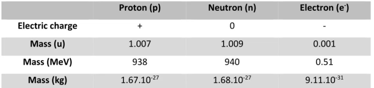
Table 3. Characteristics of the subatomic particles constituting elements in the physical universe. ... 17 Table 4. Common modes of nuclear decay (Averill and Eldredge 2012). ... 20 Table 5. Examples of 238U, 235U and 232Th natural decay chains, showing associated daughter radionuclides and
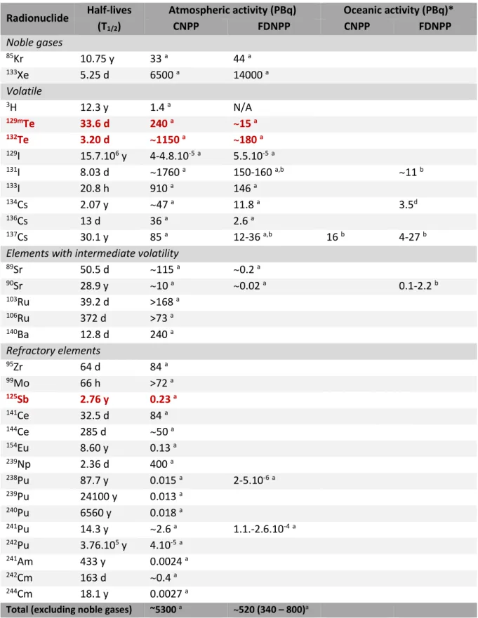
corresponding half-lives. Colours represent particle reactivity (for more information see Ah and Car 2016). ... 22 Table 6. Public exposure to natural radiation (WNA 2018) ... 23 Table 7. Comparative whole-body radiation doses and observed effects (WNA 2018) ... 23 Table 8. Nuclear power plants in commercial operation (WNA 2018)... 28 Table 9. Examples of activity levels emitted to the atmosphere and ocean after Chernobyl (CNPP) and Fukushima Daiichi (FDNPP) nuclear power plant accidents. Elements of interest for this work are highlighted (red). *1PBq = 1015 Bq ... 32
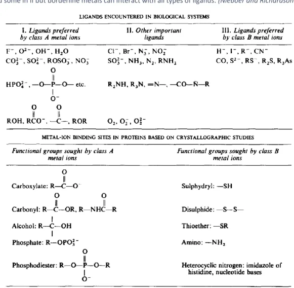
Table 10. Class A/B and borderline metal-binding ligands encountered in biological systems (upper table) and specific amino acid functional groups (bottom table). Symbol R represents any alkyl radical (e.g., CH3- ) or
aromatic moiety (e.g., phenyl ring). Class A metal ions bind preferentially to ligands in column I, class B to ligands in III and some in II but borderline metals can interact with all types of ligands. (Nieboer and Richardson 1980). ... 53 Table 11. Examples of redox reactions involved in natural diagenetic systems including Sb species (red). Reactions are presented in preferential order concerning energy consumption. (Modified from Wilson et al. 2010) ... 57 Table 12: Advantages and disadvantages of selective extraction methods in sequential vs parallel protocols ... 59 Table 13. Some examples of Sb behaviour in worldwide estuaries. Both dissolved (Sbd) trend and particulate
(Sbp) descriptions are shown when available from the same study ... 64
Table 14. Criteria for distinguishing clay minerals. (Nelson 2014) ... 110 Table 15. Biological concentrations (µg kg-1) of Te, Sb and Se in wild mussels (Mytilus galloprovincialis) from
Arriluze (N=20). Errors correspond to standard deviations (SD). Abbreviations: Limit of Detection (LOD). ... 116 Table 16. List of interferences in ICP-MS for targeted elements (Sb, Te and Se). Isotopes that were not used in this work due to low abundance or high interference effects are presented in grey font. ... 121
CHAPTER 4: Particulate carrier phases of Sb, a fractionation approach
Table 17: Summary of most commonly used reagents and identified artefacts/remarks in cation- and anion-adapted (mostly sequential) selective extractions ... 213
CHAPTER 6: Trace element reactivity of Sn and Se in contrasting
fluvial-estuarine systems – a comparative approach between the Gironde Estuary and
the Rhône River
Table 18. Analytical performance of Cs, Sn and Se in dissolved (freshwater NIST 1643f) and particulate/biological (stream sediment NCS DC 73307 and oyster tissue NIST 1566b) certified reference
limits of detection (LOD = 3·SD (n=10 blanks)). ... 323 Table 19. Total concentrations (µg kg-1) of Cs, Sn and Se in wild oysters (Crassostrea gigas, cf. Magallana gigas)
from the La Fosse (Gironde Estuary mouth, N=20) and Comprian (Arcachon Bay, N=20) sites in the Atlantic coast, as well as wild mussels (Mytilus galloprovincialis) from the St. Maries de la Mer (“Petit” Rhône River mouth, N=80) and Faraman (“Grand” Rhône River mouth, N=80) sites in the Mediterranean coast. Errors correspond to standard deviations (SD). ... 324
DISCUSSION
Table 20. Example of coupled timescales for Sb and Te radionuclide dispersion scenarios in the Gironde Estuary. Assumed solid/liquid equilibrium times (tS/L(eq)) for Te isotopes are ~5h in 1000 mg L-1 (i.e., MTZ) and ~4 days in
100 mg L-1 (i.e., average estuarine SPM), deduced from Te sorption kinetics (Chapter 5). Predicted fate is based
on a single discharge, thus, scenarios for continuous/intermittent NPP discharges would, at least partly derive from the following: ... 334
AEAG Agence de l'Eau Adour Garonne
AMORAD Amélioration des Modèles de prévision de la dispersion et d'évaluation de l'impact des RADionucléides au sein de l'environnement
ANR Agence Nationale de la Recherche
Asd/p Arsenic dissolved/particulate
BAF BioAcumulation Factor
BWR Boiling Water Reactor
Chl-a Chlorophyll a
CNPP Chernobyl Nuclear Power Plant
DOC Dissolved Organic Carbon
Eh Redox potential
POC Particulate Organic Carbon
cf. “compared to”
CRM Certified Reference Material
DIREN DIrection Régional de l'Environnement
EDF Éléctricité De France
EPOC Environnements et Paléoenvironnements Océaniques et Continentaux
ex "experimental" or spiked
FDNPP Fukushima Daiichi Nuclear Power Plant
FOREGS FORum of European Geological Surveys
FY Fission Yield
HCl Hydrochloric acid
HF Hydrofluoric acid
HNO3 Nitric acid
HOAc Acetic acid
IAEA International Atomic Energy Agency
ICP-MS Inductively Coupled-Plasma Mass-Spectrometre
IEA International Energy Agency
Ifremer L'Institut Français de Recherche pour l'Exploitation de la Mer
I'geo modified geoaccumulation Index
INES International Nuclear and radiological Event Scale IRSN Institut de Radioprotection et de Sûreté Nucléaire
Kd solid/liquid partitioning coefficient
LOD Limit of Detection
MGTS Métaux Gironde Transfert et Spéciation
MOX Mixed OXide fuel
MTZ Maximum Turbidity Zone
nat "natural" or inherited
NPP Nuclear Power Plant
PBq Peta Becquerel
pH Hydrogen potential
PWR Pressurised Water Reactor
Q water discharge
RNO/ROCCH Réseau National d'Observation/Réseau d'Observation de la Contamination Chimique du littoral
S Salinity
Sbd/p Antimony dissolved/particulate
SCHeMA integrated in Situ Chemical Mapping probes
Sed/p Selenium dissolved/particulate
Snd/p Tin dissolved/particulate
SOGIR Service d'Observation de la GIRonde
SORA Station Observatoire du Rhône en Arles
SPM Suspended Particulate Matter
Sv Sieverts
t1/2 Half-life
TCE Technology Critical Element
Ted/p Tellurium dissolved/particulate
TGM Transferts Géochimiques des Métaux à l'interface continent-océan
Thp Thorium particulate
USEPA U.S. Environmental Protection Agency
USGS U.S. Geological Survey
WHO World Health Organisation
1
I.
CONTEXT
1. Worldwide energy demand: the reason for nuclear energy production
Global development of modern socio-economies has been widely enhanced since the discovery and mastering of electricity. The use of electricity has become intrinsic to our individual daily activities to such an extent that electrical power and its availability appear as ubiquitous and granted. Accordingly, we tend to lose the awareness of our dependence on its production. Supporting evidence from the International Energy Agency (IEA) indicates that almost 40% of total electricity production worldwide is destined to residential and personal transport uses (Figure 1).
Figure 1. Worldwide largest electricity end uses (Australia, Austria, Canada, Czech Republic, Finland, France, Germany, Greece, Ireland, Italy, Japan, Korea, New Zealand, the Netherlands, Spain, Sweden, Switzerland, the United Kingdom and the United States). Other industries include agriculture, mining and construction. Passenger
cars include cars, sport utility vehicles and personal trucks (IEA 2017).
This electricity is produced from several sources which can be briefly classified into:
Fossil fuels (coal, petroleum and natural gas) and biofuels
Renewable energies: based on wind/water motion on Earth or from solar radiation
Nuclear energy (enriched radioactive materials in nuclear fission and future nuclear fusion)
Despite the different energy sources and their well-known advantages (e.g., green-technology,
continuous supply, cheap production, etc.) and disadvantages (e.g., CO2 emissions, instability for the
grid, consumable sources, etc.), the trend of worldwide electricity generation has been increasing (Figure 2a) ever since a record exists (i.e., 1970’s, IEA 2017). Noteworthy, during this time (1970’s to 2010’s) a parallel development in the nuclear energy sector has also increased, accounting in 2015 for almost 11% of the world’s electricity production (Figure 2b).
2
Figure 2. Worldwide statistics on: (a) electricity generation by fuel type (1971-2015), (b) source shares of electricity generation (1973 and 2015 as examples), (c) nuclear electricity production by region (1971-2015), and (d) outlook to 1940’s total primary energy supply by fuel type and socio-economic predicted scenario. Countries are classified according to their attachment to the Organisation for Economic Co-operation and Development (OECD; IEA 2017).
3
In fact, nuclear energy constitutes a low-cost and continuous mean for electricity generation
(WNA 2015) exempted from current large scale CO2 emission-issues (i.e., Climate Change and
consequences; IPCC 2017). Furthermore, despite the slight decrease in production in ~2011 (i.e., Fukushima Dai-ichi Nuclear Power Plant accident) followed by a current stabilisation (Figure 2c), nuclear energy is still considered an adequate alternative for future electricity demands (Figure 2d), expected to increase by more than two-thirds by 2035 (WNA 2015, 2018).
In the worldwide ranking of nuclear energy production by countries (Table 1), the United States of America are in the lead, producing ~32% of global nuclear energy (N ~100 reactors), spending <20% in domestic use (IEA 2017). The second nuclear energy producing country is France, with a global production of 17%, mostly invested in domestic use (>77%) and exportation (Table 2). This means that France is the European country with the highest local nuclear energy production, important nuclear management facilities and the highest nuclear dependence in the power supply (as nuclear energy accounts for ~75% of the total energy share; WNA 2015).
Table 1. Worldwide 2015 statistics for global nuclear energy production (left) and relevance in domestic application (right) per country (IEA 2017).
Producers TWh % of world
total Top ten countries
% of nuclear in total domestic electricity
United States 830 32.3 France 77.6
France 437 17.0 Ukraine 54.1
Russian Federation 195 7.6 Korea 30.0
China 171 6.7 United Kingdom 20.9
Korea 165 6.4 Spain 20.6
Canada 101 3.9 United States 19.3
Germany 92 3.6 Russian
Federation 18.3
Ukraine 88 3.4 Canada 15.1
United Kingdom 70 2.7 Germany 14.3
Spain 57 2.2 China 2.9
Rest of the world 365 14.2 Rest of the world* 7.2
World 2571 100 World 10.6
4
Table 2. Worldwide 2015 electricity net exporter and importer countries (IEA 2017).
Net exporters TWh Net importers TWh
France 64 United States 67
Canada 60 Italy 46
Germany 48 Brazil 34
Paraguay 41 Belgium 21
Sweden 23 United Kingdom 21
Norway 15 Finland 16
Czech Republic 13 Hungary 14
China 12 Thailand 12
Russian Federation 12 Hong Kong. China 11
Bulgaria 11 Iraq 10
Others 39 Others 112
Total 338 Total 364
2. European concern on the nuclear energy industry: a focus on radioecology
The European Research Area (ERA) was formed in 2000 to coordinate and favour European co-evolution in research-and-development (R&D) and scientific excellence, supporting several projects within succeeding Framework Programmes (e.g. FP6, FP7, H2020) on different research topics and subjects of socio-economic impact. Within the European interests, the EURATOM project was designed to coordinate the European development of the nuclear industry as, in the future, energy supply (i.e., nuclear fusion and fission), waste disposal and nuclear safety are a matter of European concern.
In standard working conditions, the population is exposed to very low ionising radiation (~0.3 µSv
y-1; 1%) coming from Nuclear Power Plants (NPPs). This contrasts with the 85% of natural background
radiation (e.g., 200 µSv y-1 from radon in houses or 1000 Bq kg-1 of granite rock) and 14% from medical
use (e.g., average 370 µSv y-1 from medical chest X-ray, corresponding to 70 million Bq; WNA 2015).
However, during NPP accidents, i.e. Chernobyl (CNPP, Ukraine 26th April 1986) and Fukushima Dai-ichi
(FDNPP, Japan 11th March 2011), atmospheric radiation levels (i.e., iodine-131 equivalent) increased
up to 5300 PBq and 520 PBq, respectively, with 20 mSv y-1 established as the maximum dose threshold
to delimit the evacuation zone in case of a FDNPP accident (Steinhauser et al. 2014; WNA 2015). These extremely high radiation levels entail potential risks in causing at long term cancers and leukaemia (mostly due to internal radioactive exposure) and relevant psychological disturbances on public health (due to lack of radiological/environmental knowledge; Steinhauser et al. 2014).
5
The use of current nuclear facilities implies the risk of potential accidents such as those of CNPP and FDNPP, with hypothetically non-negligible large-scale impacts. Nevertheless, there is still high uncertainty on radioactive environmental dispersion, activity levels and consequences for humans and organisms. For this reason, the COMET project (COordination and iMplementation of a pan-European instrumenT for radioecology) was launched within the FP7-EURATOM-Fission in 2013 to coordinate the studies on radioecology (i.e., the environmental behaviour/processes and transport of natural and anthropogenic radiation, its transfer towards organisms along the human food chains and the transgenerational effects in radiosensitive species). Such studies are a prerequisite for nuclear risk assessment, as decision making for nuclear safety requires precise knowledge on exposure pathways and environmental dispersion.
Nuclear risk assessment follows several phases at different spatial and temporal scales, applicable to all types of incidents and accidental magnitudes (Figure 3). The first phase is the crisis or emergency phase, subdivided into menace phase (anomalous event compromising environmental levels), discharge phase (external detection of radioactivity from the NPP installations) and end of the emergency phase (when the NPP installation has returned to a safe status). The second one is the post-accidental phase subdivided in the transition (first months to years, with intense measuring campaigns) and long-term phases (environmental sampling campaigns are pursued and allow, together with modelling, to achieve an increased knowledge on contamination fate). The idea is to react efficiently and in an organised manner to a nuclear release, improving actions in future events based on the knowledge from direct measurements and experiences. Such knowledge on radiological risk assessment is essential for decision making of authorities at all levels (e.g., the Nuclear Safety Authority-ASN, prefects, ministries, amongst others).
Figure 3. Spatio-temporal phases after a nuclear incident/accident. (Modified from IRSN 2014).
EMERGENCY PHASE Ti m e POST-ACCIDENTAL PHASE NPP site Near-by areas Large-scale Space Emission ↓ Internal Emergency Plan (contention) Internal repairing Dispersion ↓ Individual Intervention Plan (stable iodine intake, evacuation) Deposition ↓ Zoning decision making (defining safety zones) Lifting of emergency protection actions Population and territory management (distance to affected area, food bans,
clean-up actions) En d Di sc h ar ge M e n ac e Lo n g-te rm Tr an si ti o n
6
II.
THE RESEARCH QUESTION
1. Nuclear energy in France: current status and future plans
The French NPP network, operated by the electrical company Electricité de France (EDF), consists of 19 NPPs distributed over the metropolitan territory; 14 NPPs associated to streams and 5 NPPs located on the coast (Figure 4). There is a total of 58 pressurised water reactors (PWR; WNA 2015)
with a net total power production of ~63 GWe. Since 2005, a 59th new generation Evolutionary
Pressurised Water Reactor type (EPR) is under construction in Flamanville, expected to contribute 1.6 GWe (ANS 2016).
Figure 4. French Nuclear Power Plant (NPP) network. Range of operating starting year for all reactors per NPP (brackets). Legend shows reactor differences by energy generating capacity (Megawatts electric, MWe) and reactor characteristics: single wall lined reactor with steel sealing skin (CP0 and CPY, red), double concrete reinforcement for accident prevention (P4 and P'4, yellow), compact steam generator with higher reliance on computer software (N4, blue), and new generation reactor under construction (EPR, pink). (Modified from ANS
2016). (1988 - 1989) (1981 - 1983) (1979 - 1980) (1987 - 1992) (1984 - 1988) (2000) (2002) (1984 - 1985) (1980 - 1981) (1978) (1986 - 20XX) (1991 - 1994) (1980 - 1985) (1988 - 1989) (1985 - 1986) (1990 - 1992) (1986 - 1987) (1983) (1980 - 1981)