HAL Id: hal-00389454
https://hal.archives-ouvertes.fr/hal-00389454
Submitted on 28 May 2009
HAL is a multi-disciplinary open access
archive for the deposit and dissemination of
sci-entific research documents, whether they are
pub-lished or not. The documents may come from
teaching and research institutions in France or
abroad, or from public or private research centers.
L’archive ouverte pluridisciplinaire HAL, est
destinée au dépôt et à la diffusion de documents
scientifiques de niveau recherche, publiés ou non,
émanant des établissements d’enseignement et de
recherche français ou étrangers, des laboratoires
publics ou privés.
Hybrid Admission Control Algorithm for IEEE 802.11e
EDCA: Analysis
Mohamad El Masri, Guy Juanole, Slim Abdellatif
To cite this version:
Mohamad El Masri, Guy Juanole, Slim Abdellatif. Hybrid Admission Control Algorithm for IEEE
802.11e EDCA: Analysis. Seventh International Conference on Networking (icn 2008)., Apr 2008,
Cancun, Mexico. pp.93-98, �10.1109/ICN.2008.102�. �hal-00389454�
Hybrid admission control algorithm for IEEE
802.11e EDCA: analysis
Mohamad El Masri
University of Toulouse LAAS-CNRS Toulouse, France Email: [email protected]Guy Juanole
University of Toulouse LAAS-CNRS Toulouse, France Email: [email protected]Slim Abdellatif
University of Toulouse LAAS-CNRS Toulouse, France Email: [email protected]Abstract—One of the main Quality of Service mechanisms, allowing mainly the protection of already active flows, is ad-mission control. This is even truer on the MAC level of 802.11 based networks due to scarce resources. We present in this paper a hybrid admission control algorithm for IEEE 802.11e EDCA. The algorithm uses the synthetic Markov chain model of EDCA that we developed in previous work injecting into it network state measurements. Simulations and results presented in this paper show a good protection of admitted flows and a good utilization of the network resources.
I. INTRODUCTION
Recent advances in terms of usage of wireless networks made it essential to imbed into the access mechanisms a complete Quality of Service (QoS) architecture. IEEE 802.11e is the QoS oriented standard of amendments to be brought into IEEE 802.11. It introduces a new access function, HCF which is composed of a distributed channel access mechanism: the Enhanced Distributed Channel Access (EDCA), and a centralized, polling based access mechanism: the HCF Con-trolled Channel Access (HCCA). IEEE 802.11e sets the frame for the implementation of an admission controller within its architecture. Several admission control algorithms have been proposed in literature for both EDCA and HCCA, a review of some of them is available in [1].
The authors in [1] specify, for EDCA, two categories of admis-sion control algorithms: measurement based algorithms and model based algorithms. Measurement based algorithms take into account continuous measurements of network conditions: for example the throughput of already admitted flows, de-lays, queue size, collision conditions among others, to decide whether a new flow can be granted access to the network. In model based algorithms, network metrics drawn from analytical models are used in the decision making process. Pong and Moors [2] propose the use of the Bianchi [3] model of DCF (CSMA/CA based legacy 802.11 Distributed Coor-dination Function) to draw an achievable throughput metric of EDCA access categories. This metric is used to predict the achievable throughput of flows requesting admission and make a decision on whether the flow should be admitted or not. The use of a model in an admission control process makes it crucial for the model to be as correct and near to reality as possible. In this context, Bianchi’s model only represents the access mechanisms of one access category per station, thus lacking both the representation of the multiple access functions acting within the same station and the effective occupation of the
medium by the different access categories.
In this paper, we present a hybrid admission control algorithm using a synthetic model of an EDCA access category we presented in [4] and continuous measures of the state of the medium. The synthetic model was drawn from a new Markov chain model of an EDCA access category in saturation condition we presented in [5], introducing to existing models the virtual collision phenomenon.
The paper is organized as follows: we introduce in the fol-lowing section IEEE 802.11e EDCA’s access mechanisms and briefly present the synthetic model we presented in [4]. Section Three will detail our proposal of hybrid admission control algorithm. In section Four, simulation scenarios and results are presented. The last section presents future work and concludes the paper.
II. ASYNTHETIC MODEL OFIEEE 802.11EEDCA The hybrid admission control algorithm for EDCA we present in this paper uses a synthetic Markov chain model of an EDCA access category in saturation condition. In this section we first give a quick overview of EDCA then present the synthetic Markov chain model.
A. EDCA
The IEEE 802.11e work group [6] introduced EDCA as the QoS oriented distributed channel access. As for legacy Dis-tributed Channel Function (DCF), the channel access scheme is CSMA/CA (Carrier Sense Multiple Access with Collision Avoidance) i.e. the channel’s idleness for a certain number of time slots is detected following which a random backoff mechanism is started in order to avoid collisions. With regards to legacy DCF, EDCA introduces traffic differentiation. Four concurrent access categories (AC) with different priorities are introduced within each station. Each is characterized by its Arbitration Inter Frame Space (AIFS) and the contention window range [CWmin,CWmax]. AIFS is the number of
idle channel time slots that must be detected by the AC before being able to start the backoff procedure (waiting for a random amount of slots chosen within the contention window before being able to transmit). The values of AIFS and of the contention window range allow the prioritization of the different ACs. A Hybrid Coordinator (HC) usually located at the Access Point (AP) was introduced by the group as a centralized structure allowing different QoS mechanisms to
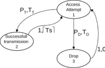
Successfull transmission 2 Access Attempt 1 Drop 3 1, Ts PT,TT PD,TD 1,0
Fig. 1. Abstract model of an EDCA AC behavior
be implemented. EDCA also defines a signaling framework used for admission control purpose.
B. Introducing the model
In [5], a Markov chain based model of the detailed behavior of an EDCA Access Category (which we call the general model), was presented. It considers a local environment (other Access Categories within the same station) and a global environment (other stations within the network). We used the Beizer rules of reduction [7] to synthesize the general model into a 3-useful state model (statistically equivalent from a user’s point of view). This synthetic model, represented in figure 1, was presented in [4]. In this section we expose the main features of the synthetic model, this model will be used within the decision making process of admission control algorithm. All the model-related expressions presented in this paper were detailed in [4].
The synthetic model is composed of three useful states: the Access Attempt state labeled 1, the successful transmission state labeled 2 and the drop state labeled 3. The Access Attempt state represents the state of an AC (which we call ACi) trying to transmit a packet (going through several
un-successful transmission attempts, the backoff times preceding those attempts and the backoff time preceding the supposedly successful transmission attempt). The successful transmission state and the drop state represent respectively the fact that a packet’s transmission was possible or not (the retransmission threshold being reached). The transitions between the states are labeled with the transition probability and the transition time (transition time from state 3 to state 1 is null, we suppose that after a packet drop, the access category proceeds instantaneously with the access attempt of a new packet). This model is a discrete Markov chain. We can evaluate by means of the transition probabilities and the transition times the equilibrium probabilities of states 1, 2 and 3: Π1,Π2and
Π3. We get Π1 = 12; Π2 = Π1PT;Π3 = Π1PD. With these
probabilities, several metrics can be computed including the throughput of the Access Category in saturation condition.
C. Needed definitions
In order to give the details of the probabilities PT and PD
and times TT and TD, we first have to specify the elements
considered in the general model of ACiaccess category [5]: A
is the number of AIFS slots of ACiN is the mean occupation
time of the medium, ⌈Ts⌉ is the smallest number of time
slots larger than the time of a successful transmission, ⌈Tc⌉
is the smallest number of time slots larger than the time of a collision, pb is the occupation ratio of the medium (i.e.
the probability for an idle medium to become busy), p(2)i
is the probability of an unsuccessful transmission attempt resulting in a ⌈Tc⌉ occupation of the medium, p
(3) i is the
probability of an unsuccessful transmission attempt resulting in a ⌈Ts⌉ occupation of the medium. Two possibilities are
represented by p(2)i : either ACi transmits (i.e. it went past
the local competition either by winning a virtual collisions or the lack thereof) and suffered a real collision, or it lost a virtual collision and the higher priority AC, winner of the virtual collision, suffered a real collision. p(3)i represents the case where ACi lost a virtual collision and the higher priority
AC, winner of the real collision, transmitted successfully. Note that pi = p
(2) i + p
(3)
i is the collision probability (be it virtual
or real) of ACi. j is the current backoff stage of ACi (i.e.
the number of transmission attempts the current packet went through). We also define Wj as the backoff stage dependant
contention window size; with 0 ≤ j ≤ m + h, due to the Binary Backoff Mechanism used within EDCA, we have, for a specified AC:
W0= CWmin
Wj+1= 2 ∗ Wj+ 1 0 ≤ j ≤ m − 1
Wm= CWmax
Wj = CWmax m≤ j ≤ m + h
Thus making m the backoff stage for which the maximum contention window is reached and m+ h the retransmission threshold for the specified AC. We also define Toas being the
mean time it takes for a backoff counter to be decremented, considering all the possible busy medium periods that can occur. We have:
To= (1 + (N + A)pb) +
PA
l=1(N + l)p2b(1 − pb)(l−1)
(1 − pb)A
D. Expressions and formulas
1) The model labels (PD ,TD,PT, TT): In figure 1, a
tran-sition is labeled with its trantran-sition probability and trantran-sition time. We will define in this section the expressions of the different times and probabilities used in the model.
a) Expressions of PD and TD: Transiting from the
awaiting transmission state to a drop state happens when a packet has suffered m+h (the retransmission threshold) failed retransmissions (i.e. m+ h + 1 collisions). This happens with a probability of PD= pm+h+1i . The time TDfor a drop is the
sum of the times of the m+ h + 1 collisions suffered by the packet and all the backoff times preceding those collisions:
TD= m+h X j=0 (TA+ (TA+ N + 1)pb 1 − pb + Tcj)
TAbeing the duration of the first AIFS period per transmission
attempt, taking into account the possible busy medium periods during the AIFS period.
TA= A − 1 +
PA−1
l=1 (N + 1)pb(1 − pb)l−1
(1 − pb)A−1
Tcj represents the duration of the backoff time before starting
a collision to which is added the collision duration. Tcj= 1 Wj+ 1 £1+W 2 j + Wj 2 To+Wj¤ + ⌈Ts⌉p(3)i + ⌈Tc⌉p(2)i pi
The drop state being, as we defined it, a virtual state, transiting back to the awaiting transmission state (i.e. dropping the current packet and considering the transmission of a new packet) happens instantaneously and deterministically.
b) Expressions of PT and TT: Transiting from the
awaiting transmission state to a successful transmission state happens with a probability PT = 1 − pm+h+1i (a packet will
eventually be successfully transmitted unless dropped). The time TT leading to this state is:
TT = 1 − pi 1 − pm+h+1i m+h X j=0 £pj i(TA+ (TA+ N + 1)pb 1 − pb + Ttj) + j−1 X l=0 (TA+ (TA+ N + 1)pb 1 − pb + Tcl) ¤
With Ttj being the duration of the backoff time preceding the
start of a successful transmission. Ttj = 1 Wj+ 1 £1 +W 2 j + Wj 2 To+ Wj ¤
2) Calculating the throughput:
a) Expressions of the achievable Throughput: From this synthetic model we deduced several performance metrics presented in [4], one of those, the achievable throughput of an Access Category if saturated, will be used in the admission decision process: when ACi’s maximum achievable
throughput is less than what it requests, new flows should be rejected. The following equilibrium state probabilities of states 1, 2 and 3: (Π1= 12;Π2= Π1PT;Π3= Π1PD) lead us to the
following formula for the throughput (note the sojourn time in state 3 is null):
T hroughputi =
Π2P ayload
Π1(PTTT+ PDTD) + Π2Ts+ Π3× 0
P ayload being the number of slots necessary to transmit the payload. Thus we finally have:
T hroughputi=
PTP ayload
PTTT + PDTD+ PT⌈Ts⌉
III. THE ADMISSION CONTROL ALGORITHM FOREDCA
A. Needed statistics and probabilities
In previous work [5], we showed that injecting to the Markov chain model of ACi measured network conditions
allows very accurate calculation of achievable throughput. We thus chose to integrate this aspect into the algorithm by collecting several statistics within the different stations of the network and within the HC. Those statistics will be used in the decision making process.
The different stations of the network must collect collision probabilities (p(2)i and p(3)i ) for each of the active flows that went through the admission control mechanism. As defined in [5], p(2)i is the ratio, to the total number of access attempts of ACi, of the number of collisions resulting in a⌈Tc⌉ occupation
of the medium, those are either real collisions of ACi (we
call this part of the ratio pir) or virtual collisions of ACi
followed by a real collisions of the AC eventually accessing the medium. p(3)i is the ratio of the number of collisions resulting in a ⌈Ts⌉ occupation of the medium to the total
number of access attempts of ACi, these represent the virtual
collisions of ACi followed by a successful transmission of
the AC eventually accessing the medium. These statistics are organized by Access Category and by ”flow using an Access Category”. They will be made available to the HC either by piggybacking or by specific management polling by the HC. The other main statistic necessary within the admission con-troller is the business ratio of medium (i.e. the probability of the medium becoming busy when originally idle). It is the job of the HC to keep track of this statistic. It must consider all the phases of a transmission attempt (regardless of its outcome) as a unique busy period of the medium.
B. Detailing the algorithm
Algorithm 1 Admission control using the synthetic model for each U pdate P eriod do
Update Busy Probabilities Update Collision Probabilities if N ew F lows6= ∅ then
Fi = Get New Flow
Update Parameters(Fi)
Calculate Achievable Throughput( Admitted F lows∪ Fi)
if Check Throughput (Admitted F lows∪ Fi) then
Admit(Fi)
Admitted F lows= Admitted F lows ∪ Fi
else
Refuse (Fi)
end if end if end for
Two main phases build up the algorithm: a continuous awareness by the HC of network condition, and a decision making process along with network condition estimation pre-sented in section III-C when a new flow arrives. The algorithm from the HC side is detailed in algorithm 1. The idea is to use the achievable throughput metric deduced from the model, injecting into it network condition through the different probabilities (pb, p
(2) i and p
(3) i ).
Each update period, which may for example be the time of a 802.11 superframe, the HC must update its vision of the network’s condition by updating the busy probability of the network (pb) and retrieving the collision probabilities of
the flows (this is done either by piggybacking during the superframe or by a direct poll of the stations at the beginning of the superframe). If a request for a new flow has arrived since the last update period, the HC calculates the achievable throughput of each of the already admitted flows and that of the new one, if the calculated achievable throughput of each flow exceeds its requested bandwidth then the newly arrived flow is granted admission, if not, the new flow will be rejected. Since the new flow has no attached information concerning its collision probabilities an estimation process described in section III-C is applied. We define two sets that will be used in the algorithm: Admitted F lows which will contain the list of already admitted flows within the network and N ew F lows in which will be saved all flows awaiting admission (i.e.
flows for which an ADDTS Request has been received but no ADDTS Response sent back). It is necessary to keep track of all already admitted flows in order to check whether admitting a new flow would degrade their achievable throughput below their requested throughput. If a flow’s specifications are to be changed (mainly due to link adaptation policies), the flow must invoke admission control before being able to transmit.
C. Enhancing the estimations
In order to better estimate the effect of accepting the new flow on active already accepted flows, it is necessary to achieve a better representation of the possible network conditions, if the new flow was to be accepted, based on the actual network conditions. This can be done by an estimation of what would be both pb and pi, based on the actual value of pb and pi.
Let Fi be the flow whose admission is being examined, Fi
will be using access category ACi in station s. We also define
τi as the probability for ACi to access the medium on a free
slot. We define Γs, the probability for station s to access the
medium. Among the access categories of a station, only one can access the medium at a time (the others are either inactive or in backoff procedure or have lost a virtual collision); we can therefore write Γs=P3i=0τi.
We defined pbas being the probability of the medium
becom-ing busy. We neglect all the reasons of business of the medium other than station access, we can therefore write
pb= 1 − (1 − Γ1)(1 − Γ2) . . . (1 − ΓM)
M being the number of stations in the medium.
pir defined earlier is the probability for ACi to suffer a
real collision when accessing the medium: ACi got past the
local competition (i.e. no virtual collisions or a won virtual collision) and went into a real collision. We can write pir as
follows:
pir= τi(1 − (1 − Γ1) . . . (1 − Γs−1)(1 − Γs+1) . . . (1 − ΓM))
In the case of the collision probability, we estimate the effect of introducing Fi on real collisions occurring on the medium.
Since we consider the admission of one flow at a time, we suppose that the access activity of Fi’s station would be the
only one to change. Let pir new and τi new be the estimated
real collision probability of ACi and its estimated access
probability if Fi was to be accepted. pir old and τi old the
actual real collision and access probabilities. We have: pir new− pir old = (τi new− τi old)(1 −
Y
j6=s
(1 − Γj))
pir new= (τi new− τi old)(1 −
Y
j6=s
(1 − Γj)) + pir old
Let ∆τ be the difference introduced by Fi to the access
category’s access probability should Fibe accepted. We have:
pir new = (∆τ)(1 −
Y
j6=s
(1 − Γj)) + pir old
This estimated ratio will be considered in the estimation of what p(2)i would be if Fi was to be admitted. Since a virtual
collision of ACi has no direct effect on the occupation of the
medium we keep both the virtual collision part of p(2)i and
p(3)i at their actual value. In the equation above, the access activities of the stations are communicated to the HC along with the information on the different active flows.
In the same fashion as above, we define pb new as the
estimated busy probability if Fi was to be accepted and pb old
the actual busy probability. Since we consider the admission of one flow at a time, we suppose that the access activity of ACi would be the only one to change. Hence:
1 − pb new 1 − pb old = (1 − Γ1)(1 − Γ2) . . . (1 − Γi new) . . . (1 − ΓM) (1 − Γ1)(1 − Γ2) . . . (1 − Γi old) . . . (1 − ΓM) = (1 − Γi new) (1 − Γi old)
Following the same reasoning as for the estimation of the real probability we have: 1 − pb new 1 − pb old = (1 − Γi new) (1 − Γi old) = (1 − Γi old− ∆τ) (1 − Γi old) 1 − pb new= (1 − pb old) (1 − Γi− ∆τ) (1 − Γi) pb new= 1 − (1 − pb old) ³ 1 − ∆τ (1 − Γi) ´
The only unknown in both estimations is ∆τ.∆τ represents
the additional accesses introduced by the new flow which can be additional transmission and possible retransmissions introduced by the flow. We use the following to estimate it: ∆τ = (1 + pir)δ, δ being the number of accesses introduced
by the flow (i.e. the number of packets to be sent during the update period). We therefore consider only one possible collision per transmitted packet. Both those estimations will be used in the calculation of the achievable throughput during the admission making process.
IV. ANALYZING THE ALGORITHM
In this section we present a simulation based analysis of the algorithm. We implemented both our algorithm and Pong and Moors’ [2] in ns-2 [8] using the module of EDCA contributed by the Telecommunication Networks Group of the Technical university of Berlin [9]. In all simulations the channel is error free, no hidden stations are present, one node is the access point in which is located the HC, all subsequently created nodes are stations (QSTA) with both active traffic generators and sinks. Access to the wireless medium is done solely using the EDCA mechanism. The stations operate at 11 Mbps data rate unless specified otherwise. We first verify the correct functioning of the admission control algorithm. The algorithm is then compared to Pong and Moors’ [2]. We chose to compare our algorithm to that of Pong and Moors because both are based on metrics drawn from Markov Chain model. We think that our model, reacting better to network condition through the integration of the busy probability of the network and thanks to the estimation we make of future network conditions will allow both a better utilization of the network and a protection of the flows.
Figure Packet Size (Bytes) Interarrival (s) Bandwidth (Mbps)
Scenario 1 600 0.003 1.6
Scenario 2 800 0.004 1.6
TABLE I
SPECIFYING THE PRESENTED SCENARIOS
A. Algorithm Verification
Simulations were performed in order to verify the well functioning of the algorithm. We analyze the decision made to accept or refuse the different flows by comparing the throughput achieved by the flows with or without admission control. We also give a view on the decision making process by comparing the estimated achievable throughput (in saturation) of the active flows to their actual throughput.
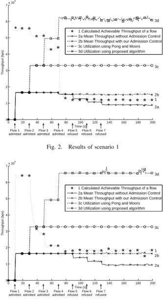
b) Simulation scenarios: The network is made up of 8 different stations, one of which is the access point (where the HC performing the admission decision process is located), the others are QSTA. In each of the 7 QSTA, a CBR flow destined to the access point is activated, the activation of the flows is made on a periodic basis. All the flows have the same requested bandwidth. Upon activation of a flow, the QSTA will send an admission control request with the different specifications of the arriving flow and will await a response before allowing or denying the flow access to the network. We investigated several different traffic specifications, with similar conclusions. We give the simulation results of some of them. Figures 2 and 3 represent the results of scenario simulations 1 and 2 respectively carried out with traffic specifications presented in table I. Note that we chose to show flows of the same bandwidth request to analyze the effect of different packet sizes on the decision making process. In each, different measured and calculated throughputs are plotted to the time of simulation, we regroup them in three groups. First group containing the graph of the calculated achievable throughput given by our proposed algorithm (labeled 1): it represents the estimation, based on the model, of the throughput an AC would achieve if saturated (when this value becomes less than the requested bandwidth of an AC, arriving flows are refused). The second group, destined to assess the protection given to the active flows, represent the mean throughput achieved by all active flows (i.e. the total throughput divided by the number of active flows) without admission control (labeled 2a) and with our proposed admission control (labeled 2b). We also represent, in a third group of plots, the network utilization (overall throughput) achieved when either Pong and Moors’ (plot labeled 3c) or our proposed algorithm (plot labeled 3d) is activated, those last results will allow us to analyze in section IV-B the performance of each admission control algorithm. Arrivals of new flows are specified by the arrows beneath the graphs along with the decision taken by the admission control algorithm we propose.
c) Results and analysis: We can see in general that the admission control algorithm intervenes to protect already active flows from arriving flows (comparing plots 2a and 2b in both figures: arriving flows are rejected when the achievable throughput becomes less than the requested bandwidth). When comparing the outcomes of simulations with similar bandwidth (comparing figure 2 to figure 3 for example), it can be
0 20 40 60 80 100 120 140 160 180 200 0 1 2 3 4 5 6 7x 10 6 Time (s) T h ro u g h p u t (b p s )
1 Calculated Achievable Throughput of a flow 2a Mean Throughput without Admission Control 2b Mean Throughput with our Admission Control 3c Utilization using Pong and Moors 3d Utilization using proposed algorithm
1 2a 2b 3c 3d Flow 1 admitted Flow 2 admitted Flow 3 admitted Flow 4 admitted Flow 5 refused Flow 6 refused Flow 7 refused
Fig. 2. Results of scenario 1
0 20 40 60 80 100 120 140 160 180 200 0 1 2 3 4 5 6 7x 10 6 Time (s) T h ro u g h p u t (b p s )
1 Calculated Achievable Throughput of a flow 2a Mean Throughput without Admission Control 2b Mean Throughput with our Admission Control 3c Utilization using Pong and Moors 3d Utilization using proposed algorithm
1 2a 2b 3c 3d Flow 1 admitted Flow 2 admitted Flow 3 admitted Flow 4 admitted Flow 5 refused Flow 6 refused Flow 7 refused
Fig. 3. Results of scenario 2
noted that the achievable throughput calculated for flows with smaller packets (therefore smaller inter arrival times) is less optimistic. This is due to several reasons: smaller inter arrival times mean more frequent accesses to the medium by each AC which means more frequent collisions. The higher collision probability is integrated into the computation of the achievable throughput, making it smaller. The other reason comes from the fact that the model considers the newly arriving flow to be saturated, thus giving a higher achievable throughput to flows with larger packets: an easy way to see this is to compare the values of achievable throughput calculated for the first flow in each simulation (at 10s in the figures), the larger the packet the higher the achievable throughput.
B. Comparison to Pong and Moors’
In this section we propose to compare the functioning of our proposed algorithm to that of Pong and Moors [2]. Using the same scenarios as earlier, we compare the network utilization achieved by both algorithms as well as the throughput achieved by the different accepted flows by one or the other algorithm.
AC Packet Size (Bytes) Interarrival (s) Bandwidth (kbps)
AC VO 400 0.032 100
AC VI 700 0.0224 250
TABLE II
SPECIFYING THE DIFFERENT FLOWS
0 20 40 60 80 100 120 140 160 180 200 0 0.5 1 1.5 2 2.5 3 3.5 4 4.5 5x 10 5 Time (s) T h ro u g h p u t (b p s )
1a Mean Throughput without Admission Control 1b Mean Throughput with proposed Admission Control 2c VO Utilization using Pong and Moors
2d VO Utilization using proposed algorithm
1a 1b 2c 2d Flow 1 admitted Flow 2 admitted Flow 3 admitted Flow 4 admitted Flow 5 refused Flow 6 refused
Fig. 4. Flows using AC VO
d) Simulation scenarios: The same scenarios above were run, using the Pong and Moors’ algorithm [2]. For each of the simulations, total utilization of the medium achieved by each of the scenarios is reported on figures 2 and 3.
e) Results and analysis: It can be clearly seen that our proposed algorithm achieves a far better utilization of the medium, while protecting already admitted flows from arriving ones. Pong and Moors’ algorithm is pessimistic: when calculating the achievable throughput of an AC, it considers all other active ACs in a saturated condition whereas our algorithm only applies the saturation condition to the AC for which the achievable throughput is being calculated. This is mainly due to the incorporation, in our algorithm, of a new metric pb, which is essential to grasp a correct view of the state
of the medium. The estimation process we apply allows our algorithm to have a better view of future network conditions.
C. Several Active ACs per station
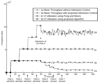
f) Simulation scenarios: Several simulations with differ-ent traffic specifications were conducted in order to observe the performance of the proposed algorithm in environments with several active ACs per station. The same network configuration as earlier is used for this simulation, the physical data rate was however reduced to 2 Mbps. This was done to reduce simulation durations, the phenomena being virtually the same with different data rates. 2 flows per station are activated, one at a time, on a periodic basis: the first using the voice access category (AC VO), the other the video access category (AC VI). The flows are described in table II.
g) Results and analysis: As with previous scenarios, we can see that our proposed admission control algorithm allows a certain protection of already admitted flows and a better utilization of the medium if compared to Pong and Moors’
0 20 40 60 80 100 120 140 160 180 200 0 5 10 15x 10 5 Time (s) T h ro u g h p u t (b p s )
1a Mean Throughput without Admission Control 1b Mean Throughput with proposed Admission Control 2c VI Utilization using Pong and Moors
2d VI Utilization using proposed algorithm
1a 1b 2c 2d Admission of VO Flow 4 Flow 1 admitted Flow 2 admitted Flow 3 admitted Flow 4 admitted Flow 5 refused Flow 6 refused Flow 7 refused
Fig. 5. Flows using AC VI
algorithm. Once again, Pong and Moors’ are too pessimistic, only one voice flow was granted access to the network (in figure 4, plots 1b and 2c overlap), whereas it was possible to allow more of them to access without jeopardizing the throughput they attain. Our algorithm attains better utilization of the network while protecting those sensitive flows.
V. CONCLUSION
In this paper we presented a new hybrid admission control algorithm. The algorithm is based on a synthetic Markov chain model we presented in [4]. Extensive simulations were carried in order to validate the algorithm. We compared the functioning of the algorithm to the model based algorithm presented by Pong and Moors [2]. The algorithm presented in this paper proved to provide protection of admitted flows while achieving a good utilization of the wireless resource. Future work is to enhance the algorithm introducing to the network condition estimation a decision-history based tuning and introducing to the algorithm delay bounds and drop probability protection.
REFERENCES
[1] D. Gao, J. Cai, and K. N. Ngan, “Admission control in ieee 802.11e wireless lans,” IEEE Network, vol. 19, no. 4, pp. 6–13, July-Aug 2005. [2] D. Pong and T. Moors, “Call admission control for ieee 802.11
con-tention access mechanism,” IEEE Global Telecommunications
Confer-ence, GLOBECOM ’03, vol. 1, no. 1-5, pp. 174–178, December 2003.
[3] G. Bianchi, “Performance analysis of ieee 802.11 distributed coordination function,” IEEE Journal on selected areas in communications, vol. 18, no. 3, pp. 535–547, March 2000.
[4] M. E. Masri, G. Juanole, and S. Abdellatif, “A synthetic model of ieee 802.11e edca,” To appear in the International Conference on Latest
Advances in Networks, ICLAN ’07, December 2007.
[5] ——, “Revisiting the markov chain model of ieee 802.11e edca and introducing the virtual collision phenomenon,” International Conference
on Wireless Information Networks and Systems, WINSYS ’07, July 2007.
[6] 802.11e, IEEE Standard for Telecommunications and Information
Ex-change between Systems – LAN/MAN specific Requirements – Part 11: Wireless LAN MAC and PHY specifications – Amendment 8: Medium
Access Control QoS Enhancements, November 2005.
[7] B. Beizer, The architecture and Engineering of Digital Computer
Com-plexes. New York: Plenum Press, 1971.
[8] “The network simulator - ns-2.” [Online]. Available: \url{http: //www.isi.edu/nsnam/ns/}
[9] “An ieee 802.11e edca and cfb simulation model for ns-2.” [Online]. Available:\url{http://www.tkn.tu-berlin.de/research/802.11e ns2/}