On the realism of the rain microphysics representation of a squall line in the WRF model. Part I: Evaluation with multi-frequency cloud radar Doppler spectra observations

(1)

HAL Id: hal-02132651

https://hal.archives-ouvertes.fr/hal-02132651

Submitted on 17 May 2019

HAL is a multi-disciplinary open access archive for the deposit and dissemination of sci-entific research documents, whether they are pub-lished or not. The documents may come from

L’archive ouverte pluridisciplinaire HAL, est destinée au dépôt et à la diffusion de documents scientifiques de niveau recherche, publiés ou non, émanant des établissements d’enseignement et de

On the realism of the rain microphysics representation

of a squall line in the WRF model. Part I: Evaluation

with multi-frequency cloud radar Doppler spectra

observations

Frédéric Tridon, Céline Planche, Kamil Mroz, Sandra Banson, Alessandro

Battaglia, Joël van Baelen, Wolfram Wobrock

To cite this version:

Frédéric Tridon, Céline Planche, Kamil Mroz, Sandra Banson, Alessandro Battaglia, et al.. On the realism of the rain microphysics representation of a squall line in the WRF model. Part I: Evaluation with multi-frequency cloud radar Doppler spectra observations. Monthly Weather Review, American Meteorological Society, 2019, �10.1175/MWR-D-18-0018.1�. �hal-02132651�

(2)

On the realism of the rain microphysics representation of a squall line

in the WRF model. Part I: Evaluation with multi-frequency cloud

radar Doppler spectra observations.

Frédéric Tridon*

Earth Observation Science, Department of Physics and Astronomy, University of Leicester, Leicester, UK. Now at: Institute for Geophysics and Meteorology, University of Cologne, Germany

Céline Planche

Université Clermont Auvergne, INSU-CNRS UMR 6016, Laboratoire de Météorologie Physique, Clermont-Ferrand, France

Kamil Mroz

National Center for Earth Observation, University of Leicester, Leicester, UK

Sandra Banson

Alessandro Battaglia

Earth Observation Science, Department of Physics and Astronomy, National Center for Earth Observation, University of Leicester, Leicester, UK

Joel Van Baelen

Wolfram Wobrock

Accepted manuscript for publication to Monthly Weather Review

(manuscript online since 13 May 2019)

(3)

Corresponding author address:

University of Leicester, University Rd, Leicester, LE1 7RH, UK

Email :

(4)

(5)

This study investigates how multi-frequency cloud radar observations can be used to evaluate the representation of rain microphysics in the WRF model using two bulk microphysics schemes. A squall line observed over Oklahoma on 12 June 2011 is used as a case study. A recently developed retrieval tech-nique combining observations of two vertically pointing cloud radars provides quantitative description of the drop size distribution (DSD) properties of the transition and stratiform regions of the squall line system. For the first time, the results of this multi-frequency cloud radar retrieval are compared to more conventional retrievals from a nearby polarimetric radar, and a supplemen-tary result of this work is that this new methodology provides a much more detailed description of the DSD vertical and temporal variations. While the extent and evolution of the squall line is well reproduced by the model, the one hour low reflectivity transition region is not. In the stratiform region, sim-ulations with both schemes are able to reproduce the observed downdraft and the associated significative sub-saturation below the melting level, but with a slight overestimation of the relative humidity. Under this sub-saturated air, the simulated rain mixing ratio continuously decreases toward the ground, in agreement with the observations. Conversely, the profiles of the mean volume diameter and the concentration parameter of the DSDs are not well repro-duced. These discrepancies pinpoint at an issue in the representation of rain microphysics. The companion paper, investigates the sources of the biases in the microphysics processes in the rain layer by performing numerical sensi-tivity studies.

(6)

1. Introduction

An accurate representation of precipitation microphysical processes is of primary importance in simulating the state of the atmosphere not only because they determine the properties of the rain falling at the ground but also because, through latent exchanges, they inﬂuence the thermodynam-ics of precipitation systems themselves, and thus their evolution. For example, Morrison et al. (2009) and Bryan and Morrison (2012) showed that the development of trailing stratiform regions in squall lines is sensitive to the representation of rain microphysics through rain evaporation.

Current mesoscale models use bulk microphysics schemes with one (e.g., Kessler 1969; Koenig and Murray 1976; Wilson and Ballard 1999) or more prognostic variables (e.g., Ferrier 1994; Feingold et al. 1998; Thompson et al. 2008; Morrison et al. 2009) to approximate and simulate the particle size distribution. Double-moment schemes are generally found to be more success-ful than one-moment ones in reproducing observations of various cloud systems (Morrison et al. 2009; Van Weverberg et al. 2012; Igel et al. 2015, and references therein). They are capable of predicting two moments of the size distributions, namely the total number concentration as well as the mass mixing ratio. As such, the double-moment schemes have more ﬂexibility in parameteriz-ing processes like raindrop breakup and self-collection which affect the number concentration but not the mixing ratio (Morrison et al. 2009; Dawson et al. 2010). There is therefore a critical need for new types of observations/retrievals having a sufﬁcient accuracy for evaluating the additional prognostic variables used in microphysics schemes (Morrison and Milbrandt 2011; Van Weverberg et al. 2012).

For example, within an idealized framework, Dawson et al. (2010) studied the differences in evaporation and cold pool properties of a squall line simulated with a single and a triple-moment schemes. The triple-moment scheme showed clear and signiﬁcant improvements in the cold pool

(7)

and reflectivity structures of the storms thanks to a more physical representation of microphysics processes such as evaporation rate by allowing vertical variability in the concentration of the drop size distribution (DSD). However the credibility of such vertical evolution could not be corrobo-rated by observations. In Morrison et al. (2012), significant discrepancies were found between the simulated and observed DSD properties at the ground during a squall line. Misrepresentation of the raindrop breakup, and of the excessive size sorting, particularly acute in two-moment schemes (Wacker and Seifert 2001; Milbrandt and McTaggart-Cowan 2010), were suggested for explaining such discrepancies. However, the sole profiles of rain parameters observed/retrieved for their case study (radar reflectivity and median diameter) were not sufficient for unequivocally determining the cause. Later on, from simulations of an intense mesoscale convective system, Varble et al. (2014b) confirmed that excessive size sorting in double-moment schemes leads to a disproportion-ate increase of the mean raindrop diameter through the rain layer in both convective and stratiform regions. This complicated their interpretation of the model vs. observation differences, i.e., too large mean raindrop diameters and too small concentration parameters close to the surface, in par-ticular when using the Morrison et al. (2009) scheme. Therefore, these studies clearly highlighted the need of more observations of the DSD properties (in particular of the concentration parameter) aloft.

Retrievals of rain microphysics proﬁles are possible with ground-based radar observations. As in Morrison et al. (2012), polarimetric radars are widely used since they provide retrievals over large areas (Wilson et al. 1997; Bringi et al. 2009); however, only bulk properties of the DSDs are retrieved and with coarse vertical resolution, and the sensitivity to parameters such as drop concentration is generally limited. Another avenue of radar-based rain retrievals exploits the fre-quency dependence of the interaction between drops and microwave radiation and combines multi-frequency vertically pointing Doppler radar observations. In such conditions, retrievals are only

(8)

possible along a vertical profile but thanks to the relation between raindrop fall speeds and sizes, DSDs can be derived from Doppler spectra. Traditionally, dual-frequency wind profiler methods have been providing accurate retrievals in steady stratiform rain (Cifelli et al. 2000). They suffer from coarse resolution and low sensitivity in light rain but, after more than two decades of progress, they have now reached a level of quality in the drop concentration retrievals which is adequate for profile comparisons with models (Williams 2016). In Varble et al. (2014b), however, this was done only at the 2.5 km level. More recently, techniques exploiting the non-Rayleigh scattering signatures obtained with high frequency cloud radars have been developed (Kollias et al. 2002; Giangrande et al. 2012). A novel technique formulated in Tridon and Battaglia (2015) and vali-dated in Tridon et al. (2017a) shows great potential in deriving profiles of DSDs at high resolution

from the combination of radar Doppler spectra obtained at Ka(35 GHz) and W-band (94 GHz).

Multi-frequency cloud radar observations have become more and more common only in recent years, e.g., in the framework of the atmospheric research measurement (ARM) program (Mather and Voyles 2013). The ARM radars are often used in scanning mode and do not record proﬁles

continuously. Multi-frequency cloud radar proﬁles at Kaand W-band were exceptionally recorded

during the whole duration of a squall line at the Southern Great Plains (SGP) central facility on the 12 June 2011 because it was the test-phase of the newly available W-band radar. Such observations provide a unique dataset for evaluating microphysical simulations of a squall line.

The overall goal of this work is to get a clear insight into the rain microphysics properties using multi-frequency cloud radar retrievals in order to improve their representation in mesoscale mod-els, and, ultimately, to progress in forecasting precipitation. Comparing the results of two different microphysics schemes in the Weather Research and Forecasting (WRF) model (Skamarock et al. 2008), this study conﬁrms the discrepancies between observed and simulated mean raindrop

(9)

di-ameter proﬁles (Morrison et al. 2012; Varble et al. 2014b) and expands the comparison to raindrop concentration parameter proﬁles.

The paper is organized as follows: Section 2 presents the squall line event under study. Section 3 describes its microphysics properties retrieved by the recently developed dual-frequency cloud radar retrieval and compare them with a more conventional retrieval from polarimetric radars. Section 4 outlines the WRF model set-up, veriﬁes that the general dynamics and thermodynamics conditions are well reproduced in the simulations, and highlight some discrepancies in the rain microphysics properties that will be further investigated in the companion paper, Part II (Planche et al. 2019). Results are summarized in Section 5 while the appendix details the radar retrieval principle and its validation.

2. The 12 June 2011 squall line event

a. Mesoscale properties

The synoptic conditions on 11 June 2011 reveal the presence of a mid-level trough extending across northwestern United States while a mid-level ridge persisted over portions of the southern plains. Conditions were moderately moist and unstable over Oklahoma, with surface dew point

temperatures exceeding 23◦C and a convective available potential energy (CAPE) of 2502 J kg−1

(Figure 1). Combined with a southeasterly low-level ﬂow advecting moisture northward from the Gulf of Mexico, a mid-level impulse over southwestern Arizona turned toward northern New Mex-ico. This led to the development of the ﬁrst thunderstorms in southeastern Colorado at 1900 UTC on 11 June 2011, which moved southeastward toward Oklahoma and then became an organized mesoscale convective system resulting in more than 50 mm of rain accumulation over large parts of Oklahoma and Kansas (Figure 2).

(10)

b. Observations at SGP

The resulting squall line system passed over the southern great plains (SGP) ARM Central

Facil-ity from 0500 UTC to 0900 UTC on 12 June 2011, producing heavy rain peaking at 100 mm h−1at

0540 UTC and followed by more than two hours of moderate stratiform rain (Figure 3). Then, the system moved to southwestern Missouri where it dissipated at 2030 UTC on 12 June 2011. The nearby WSR-88D (National Weather Service Weather Surveillance Radar-1988 Doppler) radar at

Vance, Oklahoma (KVNX, frequency of 2.8 GHz, wavelength of≈10 cm) observed the structure

and the evolution (Figure 4a, d, g) of the squall line system, characterized by three typical regions with marked differences in the intensity of the reﬂectivity.

A large suite of radar proﬁling observations is available at the ARM SGP site: the Ka-band ARM

zenith radar (KAZR, Matthews et al. 2011), the W-band scanning ARM cloud radar (WSACR, Matthews et al. 2005) and the ultra high frequency (UHF) radar wind profiler (RWP, frequency of 915 MHz, wavelength of 33 cm, Muradyan and Coulter 1998) reconfigured in precipitation mode (Tridon et al. 2013b). All three radars captured the whole evolution of the squall line as it was passing over the site (Figures 5 and A1). In particular, the KAZR and WSACR recorded the full profiles of Doppler spectra, key inputs to the dual-frequency rain retrieval used in this work, the rationale of which is detailed in the Appendix.

In line with rain-rate measured at the ground, the time evolution of the RWP reﬂectivity ZRW P

(Figure 5a) presents a clear contrast between the leading mature convective region (CR) with mul-tiple columns of high reﬂectivity corresponding to heavy precipitation (from 0515 to 0600 UTC) and the trailing stratiform region (SR) with the characteristic bright-band (BB) highlighting the

0◦C isotherm where ice melting occurs (from 0645 to 0815 UTC). As common in squall line

(11)

lighter precipitation with lower reﬂectivity in rain and a slightly less marked BB (from 0600 to 0645 UTC). The corresponding Doppler velocity (Figure 5b) — sum of the vertical air motion and the mean reﬂectivity weighted velocity of hydrometeors — highlights the contrast between ice crystals and raindrop fall velocities in the SR and the TZ, while some strong and alternating updrafts and downdrafts are present in the CR up to 12 km.

Thanks to their peculiar mesoscale structure with these three regions of disparate microphysical regimes, squall lines have been widely used for analyzing the variability of the DSDs (Maki et al. 2001; Uijlenhoet et al. 2003) and to assess models performances against observations (Bryan and Morrison 2012; Morrison et al. 2012; Morrison et al. 2015). Figure 6a shows the time evolution of the DSDs retrieved at the lowest range gate (300 m AGL) from the combination of KAZR and WSACR observations (details in the Appendix). No disdrometer observations were available for this particular case study. Nevertheless, a comparison of the corresponding rain-rate with collocated rain gages (Figure 3) shows good consistency over the wide range of rain-rates observed during this event. Interestingly, the optical rain gage underestimates the rain-rate in the SR, i.e. between 0700 and 0815 UTC. This suggests that its calibration may be inappropriate to the speciﬁc DSD properties encountered in the SR. Aloft, the quality of the retrievals is demonstrated in the appendix thanks to quantitative comparisons with the RWP reﬂectivity observations.

The DSD characteristics are in agreement with the standard interpretation of the microphysical processes involved in squall lines (Biggerstaff and Houze 1993; Houze 1993; Braun et al. 1996). In the CR, the growth associated with convection tends to produce the largest hydrometeors and

a wide range of raindrop sizes (median D0 and maximum Dmax diameter reach 4 and 7 mm,

respectively, Figure 6). The possible presence of a reﬂectivity minimum and weak bright-band in the TZ (Figure 5a) is well known and is caused by a smaller degree of aggregation occurring above the melting layer compared to the SR (Biggerstaff and Houze 1993; Houze 1993; Braun

(12)

et al. 1996). These studies suggested that this can be due to a mid-level downdraft and/or to a predominant presence of convectively generated dense ice particles which are less efﬁcient to aggregate than the vapor-grown ice crystals found in the SR. Another possibility could be that not much ice is sedimenting there, because large and dense particles have already fallen out while smaller or less dense particles are detrained high in the troposphere so that they do not reach the melting level until they are well behind the convective line. In Figure 6, this results in smaller drops

and a narrow DSD in the TZ (D0and Dmaxas small as 1.2 and 2.5 mm, respectively) compared to

the SR (D0and Dmaxﬂuctuating around 2 and 5 mm, respectively).

A novelty of this study is the availability of the spectral DSD evolution aloft (Figure 6b). Only the TZ and the SR vertical evolution can be described because of the full extinction of cloud

radar signals in the CR. While the vertical evolution of the DSD is signiﬁcant (e.g., D0and Dmax

generally increasing toward the ground), the differences between the TZ and the SR DSDs aloft are already evident with smaller but more numerous drops in the TZ. With the high resolution description of the vertical evolution of the rain properties, these two periods of distinct rain micro-physics, both persisting over about one hour, are a perfect testbed to assess if these observed rain microphysics are well reproduced in the mesoscale simulations.

3. Retrieved rain microphysics from radar observations

Before evaluating the rain microphysics representation in WRF, conventional polarimetric radars retrievals are compared with the recently developed multi-frequency cloud radar retrievals. The

retrieved parameters of the DSD are the mean volume diameter Dm and the concentration

param-eter N₀∗(deﬁned as the intercept parameter of the corresponding exponential DSD with the same

liquid water content and Dm regardless of the shape of the observed DSD, Testud et al. (2001)).

(13)

shape of the DSD, N(D), and they are predominantly weighted by drops which contribute the most to the mass content. Their general expressions as function of N(D) are

Dm= M4 M3 (1) N₀∗= 4 4 Γ(4) M₃5 M₄4 (2)

where Miis the ith-order moment of N(D) (Testud et al. 2001).

a. Polarimetric radar retrieval

Polarimetric radars enable to retrieve parameters of rain DSDs over wide areas. When volume scans are performed, vertical proﬁles can also be reconstructed at any location. Here, the focus is on the retrievals made above the SGP site by the KVNX radar which is located at a distance of

59 km from SGP. With the highest elevation angle (20◦) pointing above the top of the system and

the lowest elevation angle (0.5◦) reasonably close to the ground (700 m AGL), this is likely to be

within the range of ideal distances for looking at vertical proﬁles with WSR-88D radars. However, this results in only 5 elevation angles covering the 3 km thick rain layer, with a resulting sampling vertical resolution of roughly 500 m but with the effective resolution due to the beamwidth being even worse (1 km).

The algorithm used to retrieve the DSD parameters from polarimetric radar observations is described in Bringi et al. (2015). It is a statistical retrieval based on disdrometer observations taken during the Midlatitude Continental Convective Clouds Experiment (MC3E) ﬁeld campaign (Jensen et al. 2016), which took place around the SGP site during the two months before this squall

line event. The parameters retrieved by this technique are N₀∗ and the median mass diameter D0

with a temporal resolution of 5 minutes (i.e. the time taken by KVNX to perform a volume scan).

(14)

this study. Accordingly, by assuming that the DSD is well represented by the normalized gamma function (Testud et al. 2001)

N(D) = N₀∗f (µ)(D/Dm)µe−ΛD (3)

whereΛ andµ are the slope and shape parameters and

f (µ) =(4 +µ)

4+µ

44

Γ(4)

Γ(4 +µ), (4)

Dm can be derived from Dm= D0(4 +µ)/(3.67 +µ). Since µ is not a retrieved parameter, a

ﬁxed value µ = 3 is chosen within the range -2 to 5 typically assumed in retrieval studies (Tian

et al. 2007; Grecu et al. 2016; Mason et al. 2017). Small differences in Dm are found if µ is

derived by using a climatologicalµ− Λ relation (Williams et al. 2014).

Despite its coarser temporal and vertical resolution, the KVNX reﬂectivity above SGP (Fig-ure 7a) is in good agreement with that of RWP, depicting a clear convective column around 0530 UTC, and a reﬂectivity minimum between 0600 and 0645 UTC. As expected, the retrieved

Dm (Figure 7b) is maximum in the CR (≈2.2 mm), minimum in the TZ (≈1.2 mm) and

inter-mediate in the SR (≈1.6 mm). Such values are very close to what has been found in the squall

line described in Morrison et al. (2012), but the contrast between each period is not as marked as

that derived by the multi-frequency retrieval (Figure 8). On the contrary, N₀∗is fairly noisy and its

TZ maximum, commonly found in disdrometer observations (Maki et al. 2001; Uijlenhoet et al. 2003), is not reproduced. Similarly, it is difﬁcult to identify any clear vertical variation neither for

Dmnor for N₀∗. These limitations are related to the fact that polarimetric retrievals work best for

(15)

b. Dual-frequency cloud radar retrieval

The combination of vertically pointing Ka and W-band radars enables the retrieval of DSD

proﬁles. In fact, at these frequencies, the interaction with raindrops depends on the radar fre-quency (see Tridon et al. (2017a) and the Appendix for details). Examples of time evolution of the retrieved DSD at 0.7 and 2.5 km ASL were shown in Figure 6. From each DSD, any rain

microphysics parameter can be computed, and Figure 8 presents the time evolution of Dmand N₀∗

rain proﬁles, as well as rain mixing ratio (qr) proﬁles in order to facilitate later comparisons with

modeling results (section 4d). Vertical wind (w) proﬁles are also retrieved with an accuracy of

about 10 cm s−1(Tridon et al. 2017a). In case of heavy rain, the signal of cloud radars can be fully

attenuated rendering the dual-frequency retrieval inapplicable (e.g. see the region above 1 km in the CR and above 2 km around 0730 UTC). Note that the retrieval assumes that only rain is present in the radar volumes, which is certainly valid at least for the TZ and the SR where reﬂectivity is lower than 45 dBZ.

As expected from the DSD time evolution (Figure 6), the dual-frequency retrieval clearly

fea-tures the three squall line regions with consistent properties in each regions, both in terms of Dm

and N₀∗(Figure 8a and b). In agreement with previous disdrometer observations (Maki et al. 2001;

Uijlenhoet et al. 2003), low Dms and large N₀∗s are found in the TZ, while no particular differences

are found for mixing ratios (Figure 8c). As was already shown by Williams (2016) for another

squall line, there is some signiﬁcant vertical variation, with a clear decrease of N₀∗ and a slight

increase of Dm toward the ground. While the case in Williams (2016) has a TZ of only 5 minute

long – too short to depict any clear vertical variation, the high resolution of the current retrieval and the longer TZ duration of this case study enable a more quantitative investigation of the vertical evolution in the TZ.

(16)

c. Interpretation and comparison of averaged retrieved proﬁles

For an easier interpretation of the vertical evolution of the DSD, Dm and N0∗are averaged over

the different periods of the squall line as deﬁned in Figure 5. Since the dual-frequency proﬁles are not complete in the CR, only the TZ and the SR are further analyzed. The rain evolution as observed by radars is not in steady state. Since the averaging time is much longer than the typical fall time of the drops (according to the fall velocity-diameter relation of Atlas et al. (1973), drops

of 0.8 and 3 mm – roughly corresponding to the 10th and 90th percentile of the DSD mass in

Figure 6 – fall through the 2.5 km layer under study in 13 and 5 min, respectively), the averaged vertical proﬁle can be considered as the vertical evolution of rainfall in an average state.

Looking at the dual-frequency retrieval (black lines and grey shading in Figure 9), Dmincreases

toward the ground for both the TZ and the SR periods but at faster rate in the TZ, while N₀∗

decreases in the TZ and is almost constant in the SR. For heavy rain and when breakup and self-collection of raindrops are the dominant microphysics processes (i.e., with negligible conden-sation/evaporation and under no wind shear), many theoretical studies (Hu and Srivastava 1995; McFarquhar 2004) have suggested that the DSD tends toward an equilibrium with an exponential

tail at large sizes with a ﬁxed slope. Numerous observations suggest a slope of 2.0-2.2 mm−1, i.e.

a Dm of roughly 1.8-2 mm under the assumption of an exponential DSD. For moderate rain-rates

similar to those under consideration in this work, Barthes and Mallet (2013) have shown that,

while the equilibrium DSD is never reached, Dms of the simulated DSDs always evolve toward

the equilibrium value. The SR DSD is closer to this equilibrium already at the highest level of the retrieval just below the melting layer (lying between 3.5 and 4.1 km). This is probably a direct consequence of the snow size distribution properties, rather than a quick evolution of the SR DSD towards the equilibrium in the few hundred meters thin rain layer just below the melting layer

(17)

where the retrieval is not applicable. Conversely, with a higher concentration of drops (and hence more drop interactions), it seems plausible that the TZ DSD evolves quicklier toward the equi-librium than the SR DSD between 3 and 1 km. Therefore, even though this is an oversimplified interpretation, the dual-frequency retrieval features fine details of the DSD vertical profile in this squall line, which are compatible with our common understanding of DSD evolution.

Averaged retrievals from the polarimetric radar (red lines end errorbars in Figure 9) differ sig-niﬁcantly from the dual-frequency retrieval. This suggests that the polarimetric retrieval smooths

Dmvariations, both in the vertical and between the TZ and the SR region. Contamination by the

bright-band can explain some of the discrepancies at 3 km (a closer look at Figure 7 suggests that

Z and Dmseem to be indeed often larger at this level). The averaged N0∗proﬁle of the polarimetric

retrieval for the TZ and the SR are very similar and they lie in the middle of the range of the dual-frequency retrieval, suggesting again that the polarimetric retrieval smooths the DSD varia-tions. Several reasons can explain why the polarimetric retrieval provides limited details of the rain microphysics:

• Since the proﬁle is reconstructed from a volume scan, the vertical resolution is very coarse. • Such moderate rain-rates (in particular in the TZ) do not correspond to the range of best

performances for polarimetric radars retrievals, and noisy measurements of reﬂectivity and differential reﬂectivity can only lead to noisy retrievals.

• The DSD parameters are retrieved from the polarimetric radar observables based on an

algo-rithm adjusted from few convective case studies (Bringi et al. 2015). The bias observed in the SR may be due to the fact that the derived statistical relations are not so well representative of stratiform rain.

(18)

• The retrieval quality can be affected by non uniform beam ﬁlling (Ryzhkov 2007) because of

large sampling volumes (the polarimetric radar has a much larger beamwidth than the cloud radars and retrievals are made at a much further distance from the radar).

The polarimetric radar retrievals are unrivaled for providing the DSD properties over wide ar-eas, including heavy rain, and can be used for various application like assimilation in numerical weather prediction models or assessment of mesoscale simulations. However, these results sug-gests that, when detailed observations are needed for microphysics processes studies (like in Mor-rison et al. 2012), it would be advantageous to rather use retrievals from vertically pointing cloud radars. While the counter-argument could be centered on their limitation to moderate rain-rates and their representativeness, proﬁlers observations have indeed been successfully used for model evaluation in some previous studies (Varble et al. 2014b).

This is the first time that the polarimetric and dual-frequency cloud radar retrieval are being compared: while the comparison should be extended to a much larger dataset (including compar-isons with disdrometer), this work suggests that the accuracy of polarimetric retrieval may not be sufficient when looking at fine-scale microphysics properties.

4. Numerical simulations of the squall line system

a. Model description

Simulations of the squall line were done using the compressible, non-hydrostatic advanced Re-search Weather ReRe-search and Forecasting model (WRF) version 3.6.1 (Skamarock et al. 2008). For this study, the simulations use the following set of parameterizations: the longwave and shortwave radiation follow, respectively, the RRTM scheme based on Mlawer et al. (1997) and the Dudhia scheme (Dudhia 1989); the surface layer scheme (the revised MM5 Monin-Obukhov scheme

(19)

de-scribed in Jim´enez et al. (2012)); the Uniﬁed Noah land surface model (Chen and Dudhia 2001); the YSU boundary layer (Hong et al. 2006) and the microphysics schemes either from Morrison et al. (2009) or from Thompson et al. (2008).

A two-way nesting conﬁguration is used with three domains (represented in Figure 2) at increas-ing horizontal resolution: 12 km, 4 km and 1 km. In the horizontal, the domain sizes are, from the outermost to the innermost domain, 1656 km x 600 km, 1008 km x 456 km, and 384 km x 152 km. For the three domains, 72 levels, not linearly spaced to give more levels near the surface, are employed in the vertical with the model lid at about 20 km (mean vertical grid-spacing equal to 250 m). The larger domain is initialized on 11 June 2011 at 0000 UTC and forced every 6 hours with the Era-Interim operational reanalyzes (Dee et al. 2011) from the European Center for Medium-range Weather Forecasts. The different simulations last 36 hours.

The model settings described above provide control simulations (in contrast with the sensitiv-ity studies performed in Part II, Planche et al. (2019)) which will be referred to as MORR-CTL and THOM-CTL for Morrison et al. (2009) or Thompson et al. (2008) microphysics schemes, respectively.

b. Evolution and structure of the simulated squall line

In WRF, the radar reﬂectivity is calculated assuming Rayleigh scattering (radar wavelength much larger than the hydrometeor sizes) via the integration of the size distributions of each hy-drometeor category (Smith 1984). It can therefore be compared with low frequency rain radars such as the the WSR-88D and the ARM UHF RWP. Note however that important assumptions are made in WRF on the mass-size relation of ice species and on the shape of hydrometeors which are considered spherical. This is why no quantitative or statistical comparison are attempted: only signiﬁcant differences (of the order of 10 dB) are discussed in the following.

(20)

Comparison of the temporal and spatial evolution of the modeled reﬂectivity (with the KVNX S-band radar reﬂectivity, Figure 4) and of the temporal evolution of the innermost domain-averaged surface rainrate (with the hourly instantaneous precipitation retrieved from the S-band rainfall radars of the US NEXRAD network (Kirstetter et al. 2015), Figure 10) show that the extent and timing of the squall line are fairly well reproduced. A delay of about one hour is visible, but this is rather small knowing that the system is initiated at around 1900 UTC on the 11 June 2011 in the southern Colorado, i.e. several hundred of kilometers away.

Figure 4 also shows that the internal structure is reasonably well reproduced with a leading convective line followed by trailing stratiform precipitation. One notable difference however is that the transition zone is only somewhat visible in the MORR-CTL simulation and nonexistent in the THOM-CTL simulation. Furthermore, some major differences are observed in a more quantitative sense: 1) the average rain-rate peak is significantly overestimated by both simulations; 2) the reflectivity of the convective line is rather well reproduced in THOM-CTL (even though this is slightly masked by the absence of the transition zone) but it is way too high in MORR-CTL. These findings are confirmed when looking at the temporal evolution of the radar reflectivity profiles simulated by MORR-CTL and THOM-CTL at a specific location. For qualitative com-parisons with the RWP reflectivity, Figure 11 shows examples of such cross sections close to the ARM SGP Central Facility. In both simulations, the leading convective line has a delay of about one-hour (Figure 5). The subsequent stratiform region is slightly too short in MORR-CTL and slightly too long in THOM-CTL. Since a model cannot be expected to reproduce observations at one location, several vertical cross sections obtained at different positions (see crosses in Fig-ures 4e) are shown in the supplementary FigFig-ures 1 and 2. While the different cross sections show some variability, a leading convective cell with trailing stratiform precipitation of comparable du-ration is always found. As expected, the properties of the convective cells (such as their dudu-ration

(21)

or the highest altitude of the 50 dBZ level) are highly variable in space. Nevertheless, several features are found to be common for stratiform parts of most cross sections:

• Similarly to previous work on intense convective systems (Lang et al. 2011; Fan et al. 2017;

Varble et al. 2014b), the ice reﬂectivity is largely overestimated by MORR-CTL in the strat-iform part. Various explanations of this high bias have been found in literature: Lang et al. (2011) assumed that it was driven by wrong proportions of the different ice categories while Varble et al. (2014a) found that too strong simulated deep convective updraft produced too much condensate aloft, but also suggested that the lower exponent parameter of the snow cat-egory in the Thompson et al. (2008) scheme (the snow mass is assumed to be proportional to

D1.9as snow observations suggest, instead of D3) could explain its better performances. This

will be further explored in part II in view of the comparisons of the simulated ice and graupel mixing ratios with the retrieved ice water contents from the ARM wind proﬁler.

• Likewise, the bright band reﬂectivity is largely overestimated in MORR-CTL whereas it

ap-pears too thin in THOM-CTL. Since both schemes use the same assumptions to compute the radar reflectivity of partially melted ice (Thompson, 2018, personal communication), i.e. the approach described in Blahak (2007), this can only be explained by a different partitioning between the ice categories and/or by the different assumptions on the ice species (e.g. the mass-size relation used for snow) in each scheme. While other models can predict or diag-nose the liquid fraction of melting hydrometeors (Ferrier 1994; Walko et al. 1995; Loftus et al. 2014; Planche et al. 2014; Xue et al. 2017), the computation of partially melted ice reflec-tivity is challenging and requires a large number of assumptions such as on the air-water-ice mixture. Therefore, it is not a surprise that WRF is not able to reproduce the melting layer reflectivity in the current case.

(22)

• As in Varble et al. (2014b), rain reﬂectivities in the stratiform part are overestimated by

MORR-CTL while they are quite well reproduced by THOM-CTL.

• Regarding the TZ, a reﬂectivity minimum is observed above the melting level for

MORR-CTL but neither of the simulations is able to reproduce the clear one hour long rain reﬂectivity weakening transition zone of the observations. Even though mesoscale simulations are able to produce a TZ in idealized frameworks (Morrison et al. 2012), it is well known that it is often challenging in real cases (Fan et al. 2017; Jensen et al. 2018) as a result of the complex interplay between 3-D dynamics and ice properties.

It is not realistic to make a point to point quantitative evaluation of the 3-D dynamics of the simulated squall line, in particular within the convective region. However, 3-D winds in squall lines are generally consistent in the along-line direction and qualitative comparisons at a single location can further confirm if the 3-D structure of the squall line is sensible. 3-D wind retrievals are performed over SGP using the multi-Doppler technique (Shapiro et al. 2009; Potvin et al. 2012) by combining the three nearby WSR-88D radars KVNX, KINX and KTLX. The results are compared in Figure 12 with the simulated 3-D wind profiles close to SGP (at the location where the reflectivity fields of Figure 11 have been derived). Observations and simulations show the typical characteristics of squall line dynamics (see e.g. Braun and Houze 1994).

• Strong wind shear is present ahead of the rain-rate peak at the ground (again with a one hour

delay in the simulation), with southerly winds at low level (2 km) gradually turning toward westerly winds at 10 km. In the model however, the altitude of the shear layer appears slightly too low (around 7 km instead of 9 km) and the intensity of the shear is overestimated because of too weak winds below 7 km.

(23)

• A lower level rear inﬂow circulation is revealed by a larger eastward component of the winds

close to the surface after the rain-rate peak.

• An upper level weak ascent is associated with a front to rear circulation, as highlighted by

the reduced eastward component of the winds after the rain-rate peak. One major difference is that the northward component of the wind in this zone is much larger in the observations than in the simulations.

• Observed and simulated vertical winds properties are similar after the rain peak with a weak

mesoscale updraft and downdraft above and below 4 km respectively. Note however that the

error of the retrievals is of the order of 2 m s−1(Potvin et al. 2012).

In summary, the comparison of observed and modeled reflectivity and dynamics shows that the WRF simulations are able to reproduce the structure and evolution of the squall line, i.e. a mature squall line with a leading convective line followed by widespread stratiform precipitation. One major difference is the inability of the model to reproduce the transition zone between these two regions, a known issue which is not addressed in this study. Focusing on the stratiform region, its duration and associated 3-D winds are quite well reproduced while reflectivity comparisons confirm previous findings with a tendency to overestimation in the MORR-CTL simulation, in particular in the ice phase. Before assessing the microphysics properties of rain in the stratiform region, quantitative comparisons of the vertical wind and of the relative humidity will be performed in the following section.

c. Statistical analysis of the dynamics and thermodynamics properties within the stratiform region

The instrumentation available at the SGP site can be used to quantitatively compare the simu-lated dynamics and thermodynamics in the stratiform region. The vertical wind obtained from the

(24)

DSD retrieval (Figure 8d) and the relative humidity retrieved by the ARM Raman lidar are relevant in this context.

Comparison of model results with proﬁling observations are challenging because a model cannot be expected to reproduce exact system evolution in space and time, and the representativeness of a single event time-height is unknown. One solution is to compare statistically the observations at SGP to a large number of model columns over the whole simulated squall line. For this aim, 20 vertical cross sections (such as those in Figure 11 and supplementary Figures 1 and 2) are obtained from different positions within the squall line. From those cross sections, in order to mimic the properties of the observed SR in Figure 5a and 8d, all the stratiform regions are detected as contiguous regions with the rain reﬂectivity at 2 km higher than 30 dBZ and the rain

rate lower than 20 mm h−1. Since the main objective of this study is not to understand why the

simulations cannot reproduce the TZ, these columns are then combined disregarding their distance from the convective line. For any modeled parameter, this forms a distribution of more than 100

samples from which the median and the ﬁrst and third quartiles can be computed. Note that

this representation was chosen for its readability but another solution would be to compare the observed median proﬁle to the ensemble of median proﬁles of the 20 modeled cross sections.

Following this procedure, Figure 13 compares the profile of the vertical wind simulated with MORR-CTL (panel b) and THOM-CTL (panel c) to the profile of the retrieved vertical wind distribution (panel a) obtained from the data of Figure 8d. Because it has a much higher temporal resolution than the cross sections obtained from the model, the unique cross section of the retrieved vertical wind at SGP has a slightly larger number of samples. With no surprise, the distribution of the retrieved vertical wind contains more extreme values since the sampling volume of the cloud radars is much smaller than the size of the model box. Nevertheless, the median and quartiles of the retrieved and modeled vertical wind profiles are in good agreement and confirm a weak

(25)

downdraft over the whole rain layer (with vertical wind close to 0 m s−1 near the ground and as

low as -0.5 m s−1 at 3 km height).

Because of this mesoscale downdraft, the stratiform part in squall lines is known to be par-ticularly dry. This can be checked following the same procedure for the observed and modeled relative humidity (RH). In this case, standard measurements by radiosoundings do not bring much information on RH in the stratiform part of the squall line because they were launched at 0522 and 1728 UTC, i.e. just before the rain onset and more than 8 hours after the rain stopped, respectively. On the contrary, at the SGP site, Raman lidar observations continuously provide high resolution retrievals of RH profiles (Turner et al. 2002; Flynn et al. 2016). The structure of the retrieved RH (Figure 14) is sensible throughout the squall line, with e.g. values approaching 100% at 0500 UTC and 2 km where the presence of a cloud prevents any retrieval at higher altitudes because of the complete extinction of the lidar backscatter. Elsewehere, the signal to noise ratio is high enough to provide a spatially coherent RH up to about 2.5 or 3 km, apart from the profile retrieved during the CR whose variability make it questionable. This retrieval is an official ARM value added product which has been widely used during the last couple of decades (Turner et al. 2016, and references therein). Errors in the RH retrieval of the order 10% are expected during daytime due to high solar background levels (Turner and Goldsmith 1999). However, rainy conditions are not ideal for lidar observations and it is preferable to verify the quality of these retrievals via comparisons with mea-surements at the surface and on top of a 60 m tower (Figure 15). At the exception of the period of heavy rain where accurate RH measurements are not surprisingly challenging with any type of instrument, the Raman lidar retrievals at the lowest range gate (purple line) are in agreement with the tower measurements (yellow line) within about 10% of RH overall, and up to 20% in some parts of the TZ and the SR. This is confirmed by the comparisons of the retrieval and radio sounding measurements at 1 km (green line and black circles). Finally, the measurements taken at

(26)

the three levels of the meteorological tower (ground, 25 and 60 m) show that RH increases toward the ground in the SR, a feature that the Raman lidar retrieval is able to reproduce. In summary, the retrieval suggests a consistently dry atmosphere during the TZ and the SR with values as low as 40% between 1 and 3 km ASL (Figure 14).

Because the resolution of the Raman lidar retrieval is 10 min, only 8 profiles are retrieved within the SR. Hence, their distribution is not very instructive and only their median is compared with the median modeled RH in Figure 16 (the spread of the observations must be interpreted with caution because it is probably not representative). While retrieved and simulated profile agree on a min-imum RH situated between 1.5 and 2 km height, the simulated RH is significantly overestimated by more than 10%, with a minimum RH of 55% at 1.5 km for MORR-CTL and 60% at 1.9 km for THOM-CTL.

d. Statistical analysis of the rain microphysics properties in the stratiform region

Following the methodology of the previous section, the proﬁles of the simulated rain mass

mix-ing ratio qr, mean volume diameter Dmand concentration parameter N0∗are statistically compared

with the retrieved ones in Figures 17, 18 and 19, respectively. Note that it was decided to compare

N₀∗because it was directly provided by the retrievals but a comparison could have been done

equiv-alently on the number concentration, Nr, – usually employed in modeling studies – since these two

parameters are directly related via the relationship N₀∗= 4Nr/Dmfor exponential distribution.

The median retrieved qr proﬁle shows a continuous decrease from 3 km down to the ground.

This is consistent with active evaporation within this dry layer. This behavior is impressively well reproduced by both microphysics schemes with a slight shift of the whole MORR-CTL

pro-ﬁle toward smaller values. Despite this very good agreement in qr, the Dm and N₀∗ proﬁles are

(27)

The MORR-CTL simulation shows a strong increase of Dmtoward the ground which is not seen

in the observations as it was already found by Morrison et al. (2012) and Varble et al. (2014b).

As noticed by Varble et al. (2014b), Dmlargely exceeds the value of the equilibrium DSD (2 mm,

see section 3c) as it approaches the ground. A novelty of the current work is the evidence that

this is compensated by an excessive decrease of N₀∗. Several factors can explain such a behavior:

uncontrolled size sorting (Wacker and Seifert 2001; Milbrandt and McTaggart-Cowan 2010), an inadequate parameterization of drop breakup and self-collection, or excessive evaporation. While

higher evaporation is a candidate to explain the anomalous Dmand N₀∗proﬁles, it is not compatible

with the air being less dry in MORR-CTL than in the observations. This will be further investigated in the companion paper via sensitivity studies.

While the spread of Dm and N₀∗ in the THOM-CTL simulation is larger than in the

observa-tions with more numerous extreme values, the averaged vertical variation is comparably weak.

However, this may be the result of an artiﬁcial upper limit on Dmat 2.8 mm, which is evident in

Figure 18c. In fact, this leads to a bimodal distribution of Dmvalues and, despite an average close

to the observations, a signiﬁcant number of unrealistic Dmproﬁles are present. As it will be further

discussed in the companion paper (Planche et al. 2019), such limit is indeed used in the Thompson scheme in order to control the size sorting of raindrops.

5. Conclusions

This paper investigates how well the observed microphysic characterization of rain in the strat-iform part of a squall line can be reproduced by the WRF model with two bulk microphysics schemes. A squall line observed on 12 June 2011 over Oklahoma, for which unique dual-frequency cloud radar observations were available for the entire duration of the rain event, is used as a case study. Using the Thompson et al. (2008) and Morrison et al. (2009) microphysics schemes, the

(28)

model is able to reproduce the extent and evolution of the squall line with a leading convective line and a trailing wide stratiform region. However, both microphysics schemes fail to reproduce the one hour low reflectivity transition region observed by radars. While this comparison is primarily qualitative, the reflectivity is significantly overestimated when using the Morrison et al. (2009) microphysics scheme, confirming previous works on squall line simulations.

Such disagreement is further investigated by exploiting a recently developed retrieval technique

applied to Ka and W-band vertically pointing cloud radar observations that provides the vertical

evolution of the DSDs. The results of such retrievals are compared to more conventional retrievals from a nearby polarimetric radar. This comparison demonstrates the complementarity of these two types of retrievals, with the ﬁrst one covering extended areas but with less accuracy and the second one providing a much more detailed description of the DSD vertical and temporal variations in the transition and stratiform regions, but only for a precipitation column. The dual-frequency technique is however limited to light and moderate rainfall as cloud radars suffer from strong attenuation in heavy rain.

In the stratiform region, both simulations are able to reproduce the observed mesoscale down-draft and the associated signiﬁcative sub-saturated air mass below the melting level. However, ancillary retrieval of relative humidity with a Raman lidar (RH as low as 44%) shows that it is slightly overestimated in the simulations (55% and 60% for Morrison et al. (2009) and Thompson et al. (2008) schemes, respectively). The rain microphysics proﬁles simulated by WRF are then compared to the detailed description of DSD variability in this region. While the simulated rain mixing ratio is in good agreement with observations and shows a continuous decrease that can be

explained by evaporation in the sub-saturated air, the proﬁles of mean volume diameter Dm and

concentration parameter N₀∗are not well reproduced. The Morrison et al. (2009) scheme leads to

(29)

of N₀∗. Conversely, the Thompson et al. (2008) scheme leads to average proﬁles of Dm and N0∗

closer to the observations but with a signiﬁcantly different Dm distribution. In both case, these

discrepancies might be explained by the inadequate representation of the active rain microphysics processes (i.e., drop breakup, self-collection, evaporation or size sorting under sedimentation). They can also be partly driven by differences in the rain DSD just below the bright band, which can be related to possible model deﬁciencies in the ice phase. This will be further investigated in the companion paper via sensitivity studies.

Acknowledgments. We thank the associate editor Hugh Morrisson, Alain Protat and two other anonymous reviewers for their interesting comments which greatly helped to improve the manuscript. This work was funded by the project ”Evaluation de la Modélisation microphysique des Précipitations à l’aide d’Observations Radars Multi-fréquences (EMPORiuM)” funded by the French CNRS-INSU LEFE-IMAGO programme. This research used the SPECTRE and

ALICE High Performance Computing Facilities at the University of Leicester. The WRF

calculations have been done on French computer facilities of the Institut du Développement des ressources en Informatique Scientifique (IDRIS) CNRS at Orsay, the Centre Informa-tique National de l’Enseignement Supérieur (CINES) at Montpellier under the project 940180 and the Centre Régional de Ressources Informatiques (CRRI) at Clermont-Ferrand. The lead author is funded by the project ”Calibration and validation studies over the North Atlantic and UK for Global Precipitation Mission” funded by the UK NERC (NE/L007169/1). Data were obtained from the U.S. DOE ARM Climate Research Facility www.archive.arm.gov and from the U.S. NOAA/NSSL MRMS system available at http://mrms.ou.edu. KVNX, KINX and KTLX data were obtained from the National Oceanic and Atmospheric Administration via AmazonWeb Services (https://aws.amazon.com/noaa-bigdata/nexrad/). Their data

(30)

were ingested, edited, and analyzed using the Py-ART (http://arm-doe.github.io/pyart/), CSU RadarTools (https://github.com/CSU-Radarmet/CSU RadarTools) and MultiDop (https://github.com/nasa/MultiDop) open-source packages.

APPENDIX

General principle of the multi-frequency radar retrieval technique

a. Inﬂuence of the radar frequency on observed radar moments

Cloud radars observables (Figures A1a and A1b) provide synergistic and complementary in-formation to more conventional precipitation radars. Because of the frequency dependence of

hy-drometeor back-scattering cross sections, larger frequencies —νRW P(≈ 1 GHz) <νKa(35 GHz) <

νW(94 GHz) lead to greater sensitivities and thus can detect smaller hydrometeors (Lhermitte

1990), e.g. compare the cloud radar with RWP reﬂectivities (Figure 5a) corresponding to the ice crystals forming the ice deck between 8 and 12 km before 0500 UTC. However, attenuation by hy-drometeors generally increases with frequency leading to full extinction of the radar signal at low

levels in case of heavy rain at the highest frequencies (e.g. at 1 km and 300 m for Kaand W-band,

respectively during the most intense rainfall period at 0545 UTC). Additionally, at larger frequen-cies, the back-scattering cross section of large hydrometeors generally decreases (the so-called

non-Rayleigh effects, Tridon et al. 2013a) which also explains why ZW < ZKa < ZRW P at short

range (see e.g. at around 0600 UTC and 1 km height). Finally, the Doppler velocity (Figure A1c and A1d) highlights the contrast between ice crystals and raindrops fall velocities in the SR, and some rapidly alternating updrafts and downdrafts in the CR (mainly visible in Figure 5b because of the smaller Nyquist velocity used by cloud radars which leads to Doppler velocity aliasing (Tri-don et al. 2011)). Another consequence of the non-Rayleigh effects is that the Doppler velocity

(31)

in rain is smaller at W band (Figure A1d) because the reﬂectivity is dominated by smaller drops which fall at lower velocities.

By combining the observations from the different radars, the peculiarities observed at each dif-ferent frequency become an advantage and allow to quantitatively retrieve the hydrometeors prop-erties with an accuracy which would not be possible with a single radar. In particular, for the squall line case study presented in this work, the method of Tridon and Battaglia (2015) and Tridon et al.

(2017a) enables retrieval of DSD proﬁles from observations of Kaand W-band Doppler spectra.

b. Effect on radar Doppler spectra and DSD retrieval

Radar Doppler spectra represent the spectral reﬂectivity per bin of Doppler velocity. Thanks to the relationship between drop fall speeds and sizes, the shape of Doppler spectra obtained in a vertically pointing mode is intimately related to the particle size distribution, with the mean air motion displacing all hydrometeors equally and shifting the whole spectra along the Doppler velocity axis. On the contrary, depending on the position within the radar volume, the apparent velocity of similar sized hydrometeors can be modiﬁed differently by air turbulence, wind shear and/or cross wind, all effects adding up in the so-called spectral broadening. For these reasons, the retrieval of DSD from Doppler spectra relies on accurate estimates of spectral broadening and vertical air motion which are not realistically possible with a single frequency Doppler spectrum (Atlas et al. 1973).

At millimeter wavelength, scattering by raindrops depends on the frequency of the transmitted wave according to the Mie theory (Lhermitte 1990): the backscattering power oscillates with con-secutive maxima and minima with increasing drop size and these oscillations modulate the Doppler spectrum with the possibility of producing multi-modal spectra at W-band, with a characteristic Mie notch corresponding to drops of 1.67 mm diameter. This is demonstrated in Figures A2 and

(32)

A3 which show examples of Doppler spectra proﬁles observed by ARM Ka and W-band radars

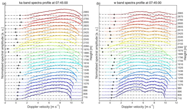
during the transition zone (at 0600 UTC) and the stratiform period (at 0745 UTC), respectively. Differences between the two radar frequencies are evident with Mie notches clearly visible in the

W-band Doppler spectra between 6 and 8 m s−1. Such differences are exploited to deduce the

vertical air motion (whose retrieved magnitude are indicated by black crosses) and the spectral broadening; then the spectral reflectivity in each Doppler velocity bin is converted into a drop concentration of the corresponding diameter. Another noticeable feature in Figures A2 and A3 is the reduction of the dynamic range of the Doppler spectra with height, especially at W-band. This is due to a lower signal to noise ratio at longer ranges because of the attenuation produced by rain and air along the path. Tangible rain attenuation is actually necessary to calibrate the spectral reflectivities and correct for possible wet radome attenuation (Tridon et al. 2017a). However, in case of heavy rain and strong attenuation, the W-band spectra have very low signal to noise ratio in the majority of the Doppler velocity bins so that the retrieval becomes inapplicable, as it is the case on the 0600 UTC profile above 2.4 km AGL (Figure A2b).

Comparing the proﬁles in Figure A2 and A3, the Doppler spectra at 0745 UTC are much wider

than at 0600 UTC – in Figure A3b, a secondary Mie notch is even somewhat visible at 9 m s−1

below 1 km (Giangrande et al. 2012) – indicating that larger drops are present in the stratiform period. This is conﬁrmed in the corresponding retrieved DSD proﬁles (Figure A4): while the DSD at 0600 UTC can be practically approximated by a piecewise linear function with a more rapid decrease in the concentration of drops larger than 1.8 mm, the DSD at 0745 UTC is almost exponential with drops as large as 5 mm. The vertical variation of the DSD corresponding to

radar proﬁles averaged over ≈2-4 s is challenging to interpret because precipitation is mainly

advected during such very short time scale. This issue can be mitigated by averaging the retrieved DSD proﬁles over a sufﬁciently long period (Tridon et al. 2017b). Both transition and stratiform

(33)

periods are long enough (60 and 85 min, respectively) to provide meaningful vertical variation of the DSD that are further exploited in this paper.

c. Validation of the DSD retrieval

An indirect validation of the retrieval is possible via the comparison of the reflectivity observed by the RWP with the Rayleigh reflectivity computed (or forward-modeled) from the retrieved DSDs (Figure A5). Because of non-Rayleigh effects and heavy rain attenuation, the reflectivity

measured by Ka and W-band cloud radars is not simply proportional to the 6th moment of the

DSD, and their reflectivity fields (Figure A1a and A1b, respectively) differ greatly from the RWP one (Figure 5a). Nevertheless and despite the large mismatch in their beamwidths, the RWP reflectivity details are very well reproduced from the DSD retrieval (Figure A5). For a more quantitative comparison, the forward-modeled reflectivity is averaged to match the resolution of the RWP reflectivity and the probability density function of their difference is shown for each range gate in Figure A6. The difference in the radar sampling volumes is large and increases with height, which explains why the reflectivity difference spread over a significant interval (-3 to +3 dB) which also slightly increases with range. On the contrary, the mean difference is lower than 0.5 dB over the whole profile (up to 3 km), which demonstrates the good accuracy of the retrieval.

References

Atlas, D., R. C. Srivastava, and R. S. Sekhon, 1973: Doppler radar characteristics of precipitation at vertical incidence. Reviews of Geophysics, 11, 1–35.

Barthes, L., and C. Mallet, 2013: Vertical evolution of raindrop size distribution: Impact on the shape of the DSD. Atmospheric Research, 119, 13–22.

(34)

Biggerstaff, M. I., and R. A. J. Houze, 1991: Kinematic and precipitation structure of the 10-11 June 1985 squall line. Mon. Wea. Rev., 119, 3034–3064.

Biggerstaff, M. I., and R. A. J. Houze, 1993: Kinematics and microphysics of the transition zone of the 10-11 June 1985 squall line. J. Atmos. Sci., 50, 3091–3110.

Blahak, U., 2007: RADAR MIE LM and RADAR MIELIB — Calculation of radar reﬂectivity from

model output. Internal Report, Institute for Meteorology and Climate Research, University of

Karlsruhe, 150 pp.

Braun, S. A., and R. A. Houze, Jr., 1994: The Transition Zone and Secondary Maximum of Radar Reﬂectivity behind a Midlatitude Squall Line: Results Retrieved from Doppler Radar Data.

Journal of Atmospheric Sciences, 51, 2733–2755.

Braun, S. A., R. A. Houze, Jr., and M.-J. Yang, 1996: Comments on ‘The Impact of the Ice Phase and Radiation on a Midlatitude Squall Line System’. J. Atmos. Sci., 53, 1343–1351.

Bringi, V. N., L. Tolstoy, M. Thurai, and W. A. Petersen, 2015: Estimation of Spatial Correlation of Drop Size Distribution Parameters and Rain Rate Using NASA’s S-Band Polarimetric Radar and 2D Video Disdrometer Network: Two Case Studies from MC3E. J. Hydrometeor., 16, 1207– 1221.

Bringi, V. N., C. R. Williams, M. Thurai, and P. T. May, 2009: Using Dual-Polarized Radar and Dual-Frequency Proﬁler for DSD Characterization: A Case Study from Darwin, Australia. J.

Atmos. Oceanic Technol., 26, 2107.

Bryan, G. H., and H. Morrison, 2012: Sensitivity of a Simulated Squall Line to Horizontal Reso-lution and Parameterization of Microphysics. Mon. Wea. Rev., 140, 202–225.

(35)

Chen, F., and J. Dudhia, 2001: Coupling an Advanced Land Surface–Hydrology Model with the Penn State–NCAR MM5 Modeling System. Part I: Model Implementation and Sensitivity. Mon.

Wea. Rev., 129, 569–585.

Cifelli, R., C. R. Williams, D. K. Rajopadhyaya, S. K. Avery, K. S. Gage, and P. T. May, 2000: Drop-Size Distribution Characteristics in Tropical Mesoscale Convective Systems. J. Appl.

Me-teor., 39, 760–777.

Dawson, D. T., II, M. Xue, J. A. Milbrandt, and M. K. Yau, 2010: Comparison of Evaporation and Cold Pool Development between Single-Moment and Multimoment Bulk Microphysics Schemes in Idealized Simulations of Tornadic Thunderstorms. Monthly Weather Review, 138, 1152–1171.

Dee, D. P., and Coauthors, 2011: The era-interim reanalysis: conﬁguration and performance of the data assimilation system. Quart. J. Roy. Meteor. Soc., 137 (656), 553–597.

Dudhia, J., 1989: Numerical study of convection observed during the winter monsoon experiment using a mesoscale two-dimensional model. J. Atmos. Sci., 46, 3077–3107.

Fan, J., and Coauthors, 2017: Cloud-resolving model intercomparison of an MC3E squall line case: Part I, Convective updrafts. Journal of Geophysical Research (Atmospheres), 122, 9351– 9378.

Feingold, G., R. Walko, B. Stevens, and W. Cotton, 1998: Simulations of marine stratocumulus using a new microphysical parameterization scheme. Atmospheric Research, 47-48, 505 – 528.

Ferrier, B., 1994: A double-moment multiple-phase four-class bulk ice scheme. part i: Description.

(36)

Flynn, C., H. Sivaraman, J. Michelsen, R. Goldsmith, R. Bambha, and R. Newsom, 2016: Atmo-spheric Radiation Measurement (ARM) Climate Research Facility. Raman Lidar Mixing Ratio (RLPROFMR2NEWS10M). 2011-06-12 to 2011-06-12, Southern Great Plains (SGP) Central Facility, Lamont, OK (C1). Accessed: 2012-01-27, Dataset available online from ARM Climate Research Facility Data Archive: Oak Ridge, Tennessee, USA., doi:10.5439/1415137.

Giangrande, S. E., E. P. Luke, and P. Kollias, 2012: Characterization of Vertical Velocity and Drop Size Distribution Parameters in Widespread Precipitation at ARM Facilities. J. Appl. Meteor.

Climatol., 51, 380–391.

Grecu, M., W. S. Olson, S. J. Munchak, S. Ringerud, L. Liao, Z. Haddad, B. L. Kelley, and S. F. McLaughlin, 2016: The GPM Combined Algorithm. Journal of Atmospheric and Oceanic

Technology, 33, 2225–2245, doi:10.1175/JTECH-D-16-0019.1.

Hong, S.-Y., Y. Noh, and J. Dudhia, 2006: A new vertical diffusion package with an explicit treatment of entrainment processes. Mon. Wea. Rev., 134 (9), 2318–2341.

Houze, R. A., 1993: Cloud dynamics. Academic Press, 573 pp.

Hu, Z., and R. Srivastava, 1995: Evolution of raindrop-size distribution by coalescence, breakup and evaporation: Theory and observation. J. Atmos. Sci., 52 (10), 1761–1783.

Igel, A. L., M. R. Igel, and S. C. van den Heever, 2015: Make it a double? Sobering results from simulations using single-moment microphysics schemes. J. Atmos. Sci., 72, 910–925.

Jensen, A. A., J. Y. Harrington, and H. Morrison, 2018: Microphysical Characteristics of Squall-Line Stratiform Precipitation and Transition Zones Simulated Using an Ice Particle Property-Evolving Model. Monthly Weather Review, 146, 723–743, doi:10.1175/MWR-D-17-0215.1.

(37)

Jensen, M. P., and Coauthors, 2016: The Midlatitude Continental Convective Clouds Experiment (MC3E). Bulletin of the American Meteorological Society, 97, 1667–1686.

Jiménez, P. A., J. Dudhia, J. F. González-Rouco, J. Navarro, J. P. Montávez, and E. Garc´ıa-Bustamante, 2012: A revised scheme for the WRF surface layer formulation. Mon. Wea. Rev., 140, 898—-918.

Kessler, E., 1969: On the continuity and distribution of water substance in atmospheric circula-tions. Meteor. Monogr., 10, 1–84.

Kirstetter, P.-E., J. J. Gourley, Y. Hong, J. Zhang, S. Moazamigoodarzi, C. Langston, and A. Arthur, 2015: Probabilistic precipitation rate estimates with ground-based radar networks.

”Water Resour. Res.”, 51, 1422–1442, doi:10.1002/2014WR015672.

Koenig, L. R., and F. W. Murray, 1976: Ice-bearing cumulus cloud evolution: Numerical sim-ulation and general comparison against observations. Journal of Applied Meteorology, 15 (7), 747–762.

Kollias, P., B. Albrecht, and F. Marks, 2002: Why Mie? Accurate Observations of Vertical Air Velocities and Raindrops Using a Cloud Radar. Bull. Amer. Meteor. Soc., 83, 1471–1483.

Lang, S. E., W.-K. Tao, X. Zeng, and Y. Li, 2011: Reducing the Biases in Simulated Radar Reﬂectivities from a Bulk Microphysics Scheme: Tropical Convective Systems. Journal of

At-mospheric Sciences, 68, 2306–2320.

Lhermitte, R., 1990: Attenuation and Scattering of Millimeter Wavelength Radiation by Clouds and Precipitation. J. Atmos. Oceanic Technol., 7, 464–479.

(38)

Loftus, A. M., W. R. Cotton, and G. G. Carri´o, 2014: A triple-moment hail bulk microphysics scheme. Part I: Description and initial evaluation. Atmospheric Research, 149, 35–57, doi:10. 1016/j.atmosres.2014.05.013.

Maki, M., T. D. Keenan, Y. Sasaki, and K. Nakamura, 2001: Characteristics of the Raindrop Size Distribution in Tropical Continental Squall Lines Observed in Darwin, Australia. J. Appl.

Meteor., 40, 1393–1412.

Mason, S. L., J. C. Chiu, R. J. Hogan, and L. Tian, 2017: Improved rain rate and drop size retrievals from airborne Doppler radar. Atmospheric Chemistry & Physics, 17, 11 567–11 589, doi:10.5194/acp-17-11567-2017.

Mather, J. H., and J. W. Voyles, 2013: The ARM Climate Research Facility: a review of structure and capabilitiess. Bull. Amer. Meteor. Soc., 94, 377–392.

Matthews, A., B. Isom, D. Nelson, I. Lindenmaier, J. Hardin, K. Johnson, and N. Bharadwaj, 2005: Atmospheric Radiation Measurement (ARM) Climate Research Facility. WBand (95 GHz) ARM Cloud Radar (WACR). 2011-06-12 to 2011-06-12, Southern Great Plains (SGP) Central Facility, Lamont, OK (C1). Accessed: 2013-06-13, Dataset available online from ARM Climate Research Facility Data Archive: Oak Ridge, Tennessee, USA., doi:10.5439/1025317.

Matthews, A., B. Isom, D. Nelson, I. Lindenmaier, J. Hardin, K. Johnson, and N. Bharadwaj, 2011: Atmospheric Radiation Measurement (ARM) Climate Research Facility. Ka ARM Zenith Radar (KAZRGE). 2011-06-12 to 2011-06-12, Southern Great Plains (SGP) Central Facility, Lamont, OK (C1). Accessed: 2012-01-27, Dataset available online from ARM Climate Research Facility Data Archive: Oak Ridge, Tennessee, USA., doi:10.5439/1025214.

(39)

McFarquhar, G. M., 2004: A New Representation of Collision-Induced Breakup of Raindrops and Its Implications for the Shapes of Raindrop Size Distributions. J. Atmos. Sci., 61, 777–794.

Milbrandt, J. A., and R. McTaggart-Cowan, 2010: Sedimentation-Induced Errors in Bulk Micro-physics Schemes. J. Atmos. Sci., 67, 3931–3948.

Mlawer, E. J., S. J. Taubman, P. D. Brown, M. J. Iacono, and S. A. Clough, 1997: Radiative transfer for inhomogeneous atmospheres: RRTM, a validated correlated-k model for the longwave. J.

Geophys. Res., 102, 16 663–16 682.

Morrison, H., and J. Milbrandt, 2011: Comparison of Two-Moment Bulk Microphysics Schemes in Idealized Supercell Thunderstorm Simulations. Mon. Wea. Rev., 139, 1103—-1130.

Morrison, H., J. A. Milbrandt, G. H. Bryan, K. Ikeda, S. A. Tessendorf, and G. Thompson, 2015: Parameterization of Cloud Microphysics Based on the Prediction of Bulk Ice Particle Properties. Part II: Case Study Comparisons with Observations and Other Schemes. J. Atmos. Sci., 72, 312– 339.

Morrison, H., S. A. Tessendorf, K. Ikeda, and G. Thompson, 2012: Sensitivity of a Simulated Midlatitude Squall Line to Parameterization of Raindrop Breakup. Mon. Wea. Rev., 140, 2437— -2460.

Morrison, H., G. Thompson, and V. Tatarskii, 2009: Impact of cloud microphysics on the devel-opment of trailing stratiform precipitation in a simulated squall line: Comparison of one- and two-moment schemes. Mon. Wea. Rev., 137, 991–1007.

Muradyan, P., and R. Coulter, 1998: Atmospheric Radiation Measurement (ARM) Climate Research Facility. Radar Wind Proﬁler (915RWPPRECIPMOM). 2011-06-12 to 2011-06-12, Southern Great Plains (SGP) Central Facility, Lamont, OK (C1). Accessed: 2012-01-27, Dataset