HAL Id: hal-00317731
https://hal.archives-ouvertes.fr/hal-00317731
Submitted on 29 Nov 2004
HAL is a multi-disciplinary open access
archive for the deposit and dissemination of
sci-entific research documents, whether they are
pub-lished or not. The documents may come from
teaching and research institutions in France or
abroad, or from public or private research centers.
L’archive ouverte pluridisciplinaire HAL, est
destinée au dépôt et à la diffusion de documents
scientifiques de niveau recherche, publiés ou non,
émanant des établissements d’enseignement et de
recherche français ou étrangers, des laboratoires
publics ou privés.
imaging Doppler interferometry (IDI) winds using the
Buckland Park MF radar
D. A. Holdsworth, I. M. Reid
To cite this version:
D. A. Holdsworth, I. M. Reid. Comparisons of full correlation analysis (FCA) and imaging Doppler
interferometry (IDI) winds using the Buckland Park MF radar. Annales Geophysicae, European
Geosciences Union, 2004, 22 (11), pp.3829-3842. �hal-00317731�
SRef-ID: 1432-0576/ag/2004-22-3829 © European Geosciences Union 2004
Annales
Geophysicae
Comparisons of full correlation analysis (FCA) and imaging
Doppler interferometry (IDI) winds using the Buckland Park MF
radar
D. A. Holdsworth1,*and I. M. Reid2
1Atmospheric Radar Systems, 1/26 Stirling St, Thebarton, South Australia, Australia
*also at: Department of Physics and Mathematical Physics, University of Adelaide, South Australia, Australia 2Department of Physics and Mathematical Physics, University of Adelaide, South Australia, Australia
Received: 28 October 2003 – Revised: 5 July 2004 – Accepted: 20 August 2004 – Published: 29 November 2004 Part of Special Issue “10th International Workshop on Technical and Scientific Aspects of MST Radar (MST10)”
Abstract. We present results from three years of meso-spheric and thermomeso-spheric wind measurements obtained us-ing full correlation analysis (FCA) and imagus-ing Doppler in-terferometry (IDI) for the Buckland Park MF radar. The IDI winds show excellent agreement with the FCA winds, both for short (2-min) and longer term (hourly, fortnightly) com-parisons. An extension to a commonly used statistical anal-ysis technique is introduced to show that the IDI winds are approximately 10% larger than the FCA winds, which we at-tribute to an underestimation of the FCA winds rather than an indication that IDI overestimates the wind velocity. Al-though the distribution of IDI effective scattering positions are shown to be consistent with volume scatter predictions, the velocity comparisons contradict volume scatter predic-tions that the IDI velocity will be overestimated. However, reanalysis of a 14-day data set suggests the lack of overesti-mation is due to the radial velocity threshold used in the anal-ysis, and that removal of this threshold produces the volume scatter predicted overestimation of the IDI velocities. The merits of using hourly IDI estimates versus hourly averaged 2-min IDI estimates are presented, suggesting that hourly es-timated turbulent velocities are overeses-timated.
Key words. Ionosphere (instruments and techniques) –
Radio science (instruments and techniques) – Meterology and atmospheric dynamics (instruments and techniques)
1 Introduction
Spaced antenna (SA) radar techniques have been used for the estimation of atmospheric wind velocities for over 60 years. “Correlation” techniques have most commonly been em-ployed, such as the “full correlation analysis” (FCA) (e.g.
Correspondence to: D. A. Holdsworth
(dholdswo@atrad.com.au)
Briggs, 1984). FCA produces two velocity estimates: the “apparent” and “true” velocities. The true velocity accounts for the effects of random changes and anisometry in the ground diffraction pattern, and is thus generally considered the better velocity estimate. Unless otherwise indicated, all references to FCA velocity hereafter refer to the true veloc-ity. The FCA also provides information on the spatial and temporal characteristics of the ground diffraction pattern. In recent years a number of “interferometric” techniques have been developed. One class of interferometric techniques con-sist of the “Doppler-sorted imaging” analyses (e.g. Adams et al., 1985; Meek and Manson, 1987; Franke et al., 1990). These analyses use cross-spectral phase information result-ing from Doppler sortresult-ing to locate discrete scatterresult-ing posi-tions for each Doppler frequency, and then combine the scat-tering positions and Doppler frequency information to deter-mine the 3-D wind velocity.
The fundamental assumption of the imaging interferomet-ric analyses is that the cross-spectral phase at each Doppler frequency bin results from a single scatterer. If two or more scatterers contribute to the same Doppler frequency bin, the resultant “effective” scattering position will not necessarily coincide with either of the actual scattering positions. The “single scatterer” situation contrasts with the “volume scat-ter” situation assumed for FCA, where scatterers are assumed to be distributed throughout the radar volume, and a poten-tially large number of scatterers contribute to each Doppler frequency bin. There has been little attempt to theoreti-cally analyze the imaging interferometric techniques due to the difficulty in theoretically modeling unsmoothed cross-spectra (e.g. Franke et al., 1990). Briggs (1995) used the FCA theoretical model to investigate the imaging interfero-metric analyses in the volume scatter situation. These in-vestigations suggested that the effective scattering positions estimated by imaging interferometry in the volume scatter situation lie along a line, and approach the zenith as the
magnitude of the turbulent motions increase. As a result, the interferometric velocity increasingly overestimates the actual wind velocity as the magnitude of the turbulent velocity in-creases (e.g. Vandepeer and Reid, 1995a). The volume scat-ter predictions of Briggs (1995) were further confirmed using a radar backscatter simulation model (e.g. Holdsworth and Reid, 1995b).
This paper describes the implementation of imaging Doppler interferometry (IDI) using the Buckland Park MF (BPMF) radar. This study was motivated both by the qual-ity of the routine IDI observations of Jones et al. (1997) and Charles and Jones (1999), and a desire to determine the ex-perimental validity of the volume scatter predictions. Sec-tion 2 discusses the imaging interferometry technique, while Sect. 3 describes the BPMF radar and IDI implementation. Section 4 presents the IDI estimated effective scattering po-sitions. Section 5 presents comparisons of the FCA and IDI results using an extension of the statistical comparison tech-nique of Hocking et al. (2001). Section 6 presents a dis-cussion of the results in terms of volume scatter predictions, while Sect. 7 presents a summary of the results. The results presented in this paper represent the longest term compari-son of IDI with any alternative wind estimation technique to date, far exceeding the four-month Dynasonde-IDI and me-teor wind comparisons of Jones et al. (2003).
2 Imaging Doppler interferometry and the volume scat-ter situation
The imaging interferometric analyses assume the cross-spectral phase at each Doppler frequency results from a single scatterer. Criteria to verify that the information at Doppler frequencies conforms with that expected from an individual scatterer have therefore been developed. The IDI technique (e.g. Adams et al., 1985; Adams et al., 1986; Bros-nahan and Adams, 1993) uses two orthogonal rows of receiv-ing antennas. Doppler frequencies exhibitreceiv-ing sufficiently lin-ear phase variation along both rows of antennas are assumed to be indicative of plane-wave incidence, and therefore dis-crete scatter. Meek and Manson (1987) assume that Doppler frequencies with simultaneous local maxima in the power-spectra for each receiving antenna are indicative of scatter from a single discrete location. Furthermore, they advocate the use of an extra receiving antenna in order to calculate the normalized phase discrepancy as a further criterion. In contrast, Franke et al. (1990) successfully applied interfero-metric analyses without use of any single scatterer criterion. The “single scatterer” and “volume scatter” situation as-sumed by the FCA represent limiting cases of the type of scattering mechanisms expected for MF radars. The vol-ume scatter predictions of Briggs (1995) suggest that the effective scattering positions (ESPs) estimated by an imag-ing interferometry lie along a line, and approach the zenith as the magnitude of the turbulent motions increase. Further, the predictions also suggest that the cross-spectral phase (or phase difference) at any Doppler frequency varies linearly
with antenna spacing. Thus, the condition of phase linear-ity along a row of antennas that is assumed to be indicative of scatter from a single scatterer (e.g. Adams et al., 1985; Adams et al., 1986; Brosnahan and Adams, 1993) is also produced in the volume scatter situation. The phase linear-ity criterion therefore does not represent an unequivocal test for scatter from a single scatterer. Based on the findings of Briggs (1995), it further follows that the interferometric ve-locity increasingly overestimates the actual wind veve-locity as the magnitude of the turbulent velocity increases (e.g. Vande-peer and Reid, 1995a). One fact that has not previously been noted to our knowledge is that the volume scatter predicted ESP azimuth (hereafter “preferred azimuth”) is equivalent to the direction of the FCA apparent velocity.
The volume scatter predictions of Briggs (1995) assume linear cross-spectral phase variation with Doppler frequency. Cross-spectral phases obtained experimentally are usually distributed about a linear variation with Doppler frequency (e.g. Holdsworth, 1997), with the “width” of this distribu-tion decreasing with increasing averaging, either in terms of Doppler frequency or time (i.e. incoherent averaging). It fol-lows that if the volume scatter predictions of Briggs (1995) are applicable experimentally, then the ESPs will be dis-tributed about the line predicted by Briggs (1995). This sit-uation was observed experimentally between 70 and 84 km using the Buckland Park MF radar by Vandepeer and Reid (1995a).
The difficulty in directly relating the volume scatter pre-dictions to experimental results led Holdsworth and Reid (1995b) to investigate imaging interferometry using a radar backscatter model (e.g. Holdsworth and Reid, 1995a). This model allows for the simulation of a range of mean wind velocities, turbulent velocities, and variable numbers of scat-terers, allowing simulations ranging from the discrete scatter situation assumed by IDI (a small number of scatterers) to the volume scatter situation assumed by FCA (a large number of scatterers). The model also allows for the verification of the ESPs, since the actual scattering positions are known. The simulated results illustrate that imaging interferometric tech-niques successfully estimate the actual scattering positions and the model input wind velocity for small numbers (from 10 to 20) of scatterers. As the number of scatterers was in-creased, the results increasingly agreed with those predicted by Briggs (1995) and Vandepeer and Reid (1995a), in that the ESPs cluster about a line along the preferred azimuth, and approached the zenith as the magnitude of the turbulent motions increase, and that the velocity increasingly overesti-mated the model wind velocity as the magnitude of the tur-bulent velocity increased.
The FCA and interferometric velocity comparisons of Holdsworth and Reid (1995b) show very good agreement with those found experimentally (e.g. Franke et al., 1990; Meek and Manson, 1987; Brown et al., 1995; Turek et al., 1995, 1998), while the ESP alignment showed similar agree-ment to that of Vandepeer and Reid (1995a) between 70 and 84 km. Despite this agreement Holdsworth and Reid (1995b) were careful not to suggest that the volume scatter
was applicable experimentally, or that the interferometric techniques would fail experimentally. However, Roper and Brosnahan (1997) and Turek et al. (1998) appear to have in-terpreted the results as implying otherwise. Quoting verba-tim from both: “Holdsworth and Reid (1995b) were unable to recover the actual scatterer positions and concluded that the scatterers identified by the IDI technique were fictitious.” The results of Holdsworth and Reid (1995b) in fact suggest this is only the case in the volume scatter situation – Fig. 2 of their paper illustrates that the actual scatterer positions are recovered reasonably well for smaller numbers of scatterers. The reference to being “unable to recover the original scat-terer” is further misleading in that it may be interpreted as implying a deficiency in the model and/or analysis used. If this was the case the actual scatterer positions would not have been recovered for a smaller number of scatterers. A further misinterpretation of the volume scatter predictions made by Turek et al. (1998) relates to their observation of a random distribution of ESPs at heights below 84 km, and evidence of a preferred azimuth of ESPs above 84 km. The preferred azimuth above 84 km was observed to not be aligned with the IDI wind direction, leading the authors to conclude that they did not find evidence of ESP alignment along the vol-ume scatter predicted preferred azimuth. However, as de-scribed above, the preferred azimuth is along the direction of the FCA apparent velocity direction, rather than the IDI velocity direction.
The actual scattering mechanism for MF partial reflections is still poorly understood (e.g. Lesicar and Hocking, 1992). The discrete and volume scatter situations are extrema, and experimental observations are most likely some combination of the two which varies according to height, season, and site. This may well explain differences observed by some investi-gators, such as the lack of overlap of the height regions where Turek et al. (1998) (above 84 km) and Vandepeer and Reid (1995a) (70 to 84 km) find evidence of preferred azimuths, despite the fact that these authors used essentially the same analysis, i.e. IDI with two perpendicular receiving antennas arms, using linear phase variation along both rows of anten-nas as a “single scatterer” criteria. Long-term comparisons, such as those presented in this paper, provide the potential to investigate scattering mechanisms, at least on the basis of height and season.
3 IDI implementation using the Buckland Park MF radar
The Buckland Park MF radar is located 35 km north of Ade-laide (34◦380S, 138◦290E), and operates at a frequency of 1.98 MHz. The antenna array consists of a 1-km diame-ter array of 89 individually accessible north-south and east-west aligned half-wave dipoles. The radar was upgraded be-tween 1991 and 1995 (e.g. Reid et al., 1995), which involved the refurbishment of the entire antenna array and the com-missioning of new transmission and radar data acquisition (RDAS) systems. The antenna array can now also be used for
TR1 TR3 TR2 TR5 TR4 T18 T8 T7 T17 T14 T15 T16 T19 T13 T12 T20 T6 T10 T9 T11 4 N o
Fig. 1. North-south antenna configuration employed for Buckland
Park MF radar from 20 December 2001 to thepresent. Each ver-tical line represents a single north-south aligned antenna. The tri-angles denote the antennas used for observations, and the appro-priate transmit channel. Antenna groups denoted TRi and Ti were
connected to transmitter i. Antenna groups denoted TRi were
con-nected to receiver i via T/R switch i.
transmission, enabling the BPMF to perform Doppler beam steering (e.g. Vandepeer and Reid, 1995a). Routine obser-vations using the refurbished radar commenced 7 May 1996 (e.g. Holdsworth and Reid, 2004). Full correlation analysis (FCA) has been applied throughout the observations, provid-ing estimates of the dynamics and the spatial and temporal properties of the radiowave scatterers (e.g. Holdsworth and Reid, 1997; Holdsworth et al., 2001). Imaging Doppler in-terferometry (IDI) was introduced on 20 August 2000. Both the FCA and IDI analyses form part of a commercially avail-able package supplied by Atmospheric Radar Systems Pty. Ltd. (ATRAD) (e.g. Holdsworth and Reid, 2004). The an-tenna configuration has been periodically modified through-out the observations to allow for implementation of differ-ent analysis techniques, and to avoid use of antennas and/or feeder cables which develop problems. The data presented in this paper were acquired using two different antenna con-figurations. The configuration shown in Fig. 1 has been used from 20 December 2001. FCA is applied to data collected using receivers 1, 2, and 3 (antenna spacings 152.3, 152.3, and 182.8 m, hereafter “FCA-small”), and 1, 4 and 5 (304.7, 318.1, and 356.6 m, “FCA-large”). IDI is applied to data collected using receivers 1, 2 and 3. The small spacing was chosen for IDI to reduce the possibility of angle of arrival (AOA) ambiguities resulting from use of spacings exceeding
Table 1. Rejection criteria for IDI analysis.
Error Explanation code
0 No error - analysis result ok. 1 Time series unsuitable for analysis
2 Fewer than three scatterers available at this height 3 Horizontal Velocity >200 m s−1
4 Vertical velocity magnitude >10 m s−1 5 Scatterer azimuth estimate not available 6 Turbulent velocity estimate not available
Fig. 2. Example of wind (red line) and scatterer azimuth (dashed
line) estimation.
The IDI analysis implemented is almost identical to that of Franke et al. (1990). The motivation for using this analysis was twofold. First, it does use “single scatterer” criterion, and therefore has no limitations regarding antenna configu-ration. Second, it yields velocities in best agreement with the FCA true velocity, whereas other IDI technique yields velocities equal to or approaching the FCA apparent veloc-ity, which is expected to overestimate the actual velocity. All Doppler frequencies with radial velocities within ±14 ms−1, AOAs within 20◦ of zenith, and powers 15 dB above the
noise floor are used in the analysis. Two-minute and hourly wind velocities are estimated. The two-minute estimates are made using AOAs and radial velocities estimated from an in-dividual two-minute data acquisition, while hourly estimates are made using AOAs and radial velocities estimates from 30 two-minute data acquisition. Hourly IDI winds can also be estimated by hourly averaging the 2-min IDI winds. Such hourly wind estimated are hereafter referred to as “hourly averaged”, while those made using 30 two-minute data ac-quisitions are referred to as “hourly estimated”. Turbulent velocities are estimated as described by Roper and
Brosna-han (1997), using a 5◦threshold, rather than 2◦. The larger
threshold used in this study is necessary since the analysis is applied using two-minute AOA skymaps, when there are oc-casionally few AOAs within 2◦of zenith. Preferred azimuths are also determined by applying a total least-squares fit to AOAs, assuming equal measurement errors in each compo-nent. The root-mean-square (RMS) zenith angle of the AOAs is also stored. The AOAs are not stored as default, but can be archived if required. The rejection criteria used are shown in Table 1. Criterion 1 rejects data where the signal am-plitude is too low, or interference is present. Criterion 2 is applied as IDI requires a minimum of three scatterers for a valid 3-D wind velocity determination. Criteria 3 and 4 reject non-sensical data. Criterion 5 indicates the preferred azimuth could not be reliably estimated. In this case all parameters other than scatterer azimuth are still valid. Criterion 6 indi-cates that a turbulent velocity could not be reliably estimated. In this case parameters other than turbulent velocity are still valid. A typical example of the ESPs and the resulting wind velocity and preferred azimuths for a 2-min record is shown in Fig. 2. In addition to the online analysed data sets, a 14-day raw data set from 19 January 2000 to 3 February 2000 has been analysed offline using the same analysis procedures to produce an additional analysed data set to the routine anal-ysed data set.
Hourly updated latest results from both the FCA and IDI analyses are available at URLs http://www.physics.adelaide.edu.au/atmospheric and http://www.atrad.com.au/results.html.
4 Effective scattering positions (ESPs)
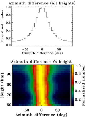
The volume scatter investigations of Briggs (1995) suggest that the ESPs should lie along a preferred azimuth, corre-sponding to the FCA apparent velocity direction. Histograms of the difference between the preferred azimuth and the FCA apparent velocity are shown in Fig. 3. These results sug-gest that the distribution of ESP azimuths is centered around the azimuth predicted by volume scatter arguments. How-ever, we note that the distribution at heights above 80 km appears to peak at negative values ≥−2.5◦, while distribu-tion at heights above 80 km appears to peak at positive values
≤2.5◦. We are not sure of the cause of this effect, but sus-pect it may be either a radar introduced bias, such as a phase calibration error. Broadening of distribution is seen around 80 km and above 90 km.
Histograms of ESPs for various height ranges from 19 Jan-uary 2000 to 3 FebrJan-uary 2000 are shown in Fig. 4. The ESPs are spread over an increasing range of zenith angles with in-creasing height, consistent with typical MF radar observa-tions that aspect sensitivity decreases with increasing height (e.g. Holdsworth and Reid, 2004). Between 90 and 100 km ESPs are observed out to 30◦, which is well beyond the trans-mit half-power half-width of ≈5◦. The distribution of ESPs is circularly symmetric, except between 60 and 70 km where the ESPs are elongated along the East-West direction. The
Fig. 3. Difference between effective scattering positions azimuth
estimated using least-squares fit and the volume scatter predicted preferred azimuth over the entire observation period.
mean FCA winds at these heights during mid-summer are strongly westerly (e.g. Holdsworth and Reid, 2004), as are the FCA apparent and IDI winds. These results therefore further support the volume scatter predictions that the ESPs lie along a preferred azimuth corresponding to the FCA ap-parent velocity direction.
5 Comparison of FCA and IDI winds
5.1 Statistical comparison technique
In order to meaningfully compare the FCA and IDI winds, we have selected four statistical indicators to assess the ve-locity components estimated by each technique. The indi-cators used are based on agreement (correlation), relative magnitude, relative variance, and data acceptance percent-age. The data acceptance percentage is defined relative to the number of data with a signal-to-noise ratio (SNR) exceed-ing −3 dB. This is used in preference to the more commonly used definition relative to the total number of time/height samples, as it is a measure of the technique itself rather than the combination of the technique, the radar system, and the atmosphere. While it is acknowledged that these indicators
may vary diurnally, seasonally, and with height, the aim of the comparisons is to provide statistics describing the tech-niques over all measurement conditions. Daily estimates of each indicator are first determined. Mean and standard devi-ations of the daily estimates are then calculated for compar-ative purposes.
The relative magnitudes of the velocity components for each technique are estimated using the statistical comparison technique of Hocking et al. (2001). This technique compares two measurements x and y of a parameter v without a-priori knowledge of system measurement errors σx and σy. The
technique does not assume that the measurement errors are contained in only one parameter, as is the case in standard least-squares estimation techniques. The technique allows for the determination of the relationship between the rela-tive magnitude (or gain) of two parameters and their mea-surement errors. The gain can only uniquely be determined if estimates of the measurement errors are known. The ob-served measurement errors contain the measurement errors specific to each measurement, and also a component related to the differences in the two techniques. For instance, for comparison of all-sky meteor and MF radar velocities the measurement error contains a component relating to the dif-ferent fields of view used by two radars. The technique as-sumes v, σx and σy are normally distributed and
indepen-dent. In the following this technique is applied to compare FCA and IDI winds. Since these winds are estimated using the same radar data the measurement errors relate to the in-dividual techniques themselves.
In order to restrict the range of possible measurement er-rors, we estimate the measurement errors of each velocity component v by determining the RMS difference between
Mtime-contiguous estimates γ = v u u t M X t =1 (v(t +1) − v(t ))2 2M , (1)
the parameter where v(t ) represents the velocity component measured at time t . This represents a measure of the root-mean-square (RMS) difference in time contiguous velocity component estimates averaged over all heights. If v is nor-mally distributed about a constant value, γ is equivalent to the root-mean-square (RMS) value of v, i.e. the measurement error of v. In the case of FCA and IDI velocity components,
v contains small (gravity wave), medium (tidal) and large (planetary wave) time-scale variations, and as such, v is not distributed about a constant value. In this case γ represents the maximum measurement error which can be attributed to the technique used to estimate the velocity component. The
γ estimates for the two parameters under comparison allow for the range of valid measurement errors to be restricted, thereby restricting the range of valid relative magnitudes. The effect of γ overestimating the measurement error is to increase the range of possible relative magnitudes that can be estimated, rather than bias the relative magnitude estimate. We note that in a small number (less than 3%) of cases the γ estimates do not yield a valid range of relative magnitudes,
Fig. 4. Histograms of effective scattering positions for 90–100 km (top left), 80–90 km (top right), 70–80 km (bottom left) and 60–70 km
(bottom right) from 19 January 2000 to 3 Februaray 2000. The dashed and dotted line indicate the transmit beam half-power half-width and twice the half-power half-width, respectively.
Fig. 5. Example of application of statistical comparison technique to FCA and IDI zonal velocities from 4 December 2002. Left: scatter plot
of FCA vs. IDI velocities. The red and green lines indicate the results of the least-squares fit, assuming all measurement errors are present in the FCA and IDI velocities, respectively. The green line indicates FCA=IDI. Right: relationship between relative magnitude and FCA and IDI measurement errors. The blue lines indicate the range of values defined by the maximum measurement error estimated. The red dotted vertical and horizontal lines indicate equal measurement errors and the corresponding relative gains, respectively.
indicating that at least one of the γ estimates actually under-estimates the measurement error σ . We believe this is the result of the data not fitting the assumptions of the analy-sis, i.e. that the parameters and their measurement errors are normally distributed. In this case, we treat the γ values as estimates of the minimum possible measurement error, and obtain a range of relative magnitudes. This may appear to be an unsatisfactory option, but we note that the mean lower and upper relative magnitude limits presented as follows are not biased by inclusion of such relative magnitude estimates. We can further refine γ by performing outlier rejection on the (v(t+1)−v(t ))2values used in Eq. (1). We also use γ as our indicator of the relative variance of each technique, but do so in the knowledge that it contains a component related to the relative magnitude of each technique.
Figure 5 shows a typical scatter plot of one day of 2-min zonal velocity components measured by FCA-large and IDI for 4 December 2002, and the relationship between the rela-tive magnitude of the IDI to FCA zonal winds and the FCA (σFCA) and IDI (σIDI) measurement errors. The correlation
between the data sets is 0.89, indicating excellent correla-tion. The relative magnitude of the IDI to FCA zonal winds is 1.12 if the FCA winds are assumed to contain no mea-surement error (i.e. σFCA=0), 1.00 if the measurement errors
are assumed to be identical (i.e. σFCA=σIDI), and 0.89 if the
IDI winds are assumed to contain no measurement error (i.e.
σIDI=0). The range of relative magnitudes does not give any
clear indication of the relationship between the techniques, given that it covers the case that IDI overestimates with re-spect to FCA, and vice versa. The γ estimates obtained us-ing this data set are σFCA=13.5 and σIDI=15.3. These values
effectively restrict the relative magnitude range from 0.97 to 0.99, allowing us to conclude (for this data set) that the FCA-large velocities are FCA-larger than the IDI velocities.
5.2 Two-minute winds comparisons
Holdsworth and Reid (2004) present comparisons of FCA winds measured using different antenna spacings with those obtained using spatial correlation analysis (SCA) and hy-brid Doppler interferometry (HDI). The results show that the FCA true velocity measured for small (large) spacings is un-derestimated by around 30% (10%). This is a consequence of the “triangle size effect” (TSE), whereby the true veloc-ity is increasingly underestimated as the spacing decreases. Because of the difficulty in theoretically analysing IDI it is not apparent whether IDI will suffer a similar bias, although Holdsworth and Reid (1995b) have shown IDI is suscepti-ble to a bias analogous to the TSE at low SNRs. Although the IDI winds described in this paper are estimated using the small antenna spacing, the aforementioned 14-day raw data set has been analysed to yield IDI winds for small (here-after IDI-small) and large (IDI-large) spacings. The statis-tical comparison of IDI-small and IDI-large velocities are shown in Table 2. The zonal winds are slightly larger at smaller spacings, and the meridional winds are slightly larger at larger spacings. We conclude from this that there is no
Table 2. Mean and standard deviation of daily relative magnitude
minima and maxima, correlation, maximum measurement errors, and acceptance percentages for IDI-large with respect to IDI-small for 19 January 2000 to 3 February 2000.
Parameter Zonal Merid.
component component Relative magnitude minimum 1.02±0.02 0.98±0.07 Relative magnitude maximum 1.03±0.02 1.00±0.02 Correlation 0.85±0.03 0.83±0.03 IDI-large measurement error, ms−1 19.1±0.3 18.5±0.5 IDI-small measurement error, ms−1 17.2±0.5 17.2±0.3 IDI-large acceptance percentage, % 99.5 99.5 IDI-small acceptance percentage, % 99.5 99.5
Table 3. Mean and standard deviation of daily relative magnitude
minima and maxima, correlation, maximum measurement errors, and acceptance percentages for IDI with respect to FCA-large for 20 August 2000 to 19 September 2003.
Parameter Zonal Merid.
component component Relative magnitude minimum 1.06±0.07 1.12±0.07 Relative magnitude maximum 1.09±0.07 1.18±0.07 Correlation 0.83±0.04 0.79±0.05 FCA-large measurement error, ms−1 12.6±1.2 12.1±1.2 IDI measurement estimate error, ms−1 12.9±1.2 12.5±1.4 FCA-large acceptance percentage, % 56.2 56.2 IDI acceptance percentage, % 95.1 95.1
convincing evidence for TSE of IDI winds. We note that the measurement errors for the smaller spacing are smaller, which is also observed for the FCA (e.g. Holdsworth, 1999b, Holdsworth and Reid, 2004). Given that the FCA-large winds are less biased than small winds, we use FCA-large winds in the following comparisons with IDI.
Table 3 shows the mean daily estimates of the four statis-tical indicators for the zonal and meridional velocity compo-nents throughout the observation period. The mean and stan-dard deviation of the daily minimum and maximum relative magnitudes are 1.06±0.07 to 1.09±0.07 for the zonal ponent, and 1.12±0.05 to 1.18±0.07 for the meridional com-ponent, indicating, the IDI winds are approximately 8−15% larger than the FCA-large winds. The correlations for both components are around 0.8, indicating very good agreement. The measurement errors for the IDI winds are approximately 20% larger. As described above, the measurement errors contain the effects of any relative magnitude differences,
Fig. 6. Zonal wind velocities estimated during daytime 4 March 2002 by FCA (top), Lataitas zero-lag CCF slope fitting correlation analysis
(middle), and IDI (bottom).
so the fact that the measurement errors exceed the relative magnitudes indicates that the measurement errors of the IDI winds are larger than the FCA-large winds. The IDI and FCA acceptance percentages are 95.1% and 56.2%, respec-tively. The IDI acceptance percentage is approximately con-stant throughout the year, while the FCA acceptance percent-ages range from 40% (equinox) to 80% (solstice).
A typical example of equinoctial daytime FCA and IDI zonal velocity estimates are shown in Fig. 6. Although the IDI results shows a larger number of successful velocity esti-mates, they also show a significant number of outliers, while
the FCA winds show very few outliers. This is because the FCA uses criteria to reject data which do not fit the model assumed by the analysis, or data that otherwise is deemed in-valid in some sense (e.g. Briggs, 1984). On the other hand, the IDI analysis only rejects data if the analysis cannot be performed (criteria 1 or 2) or if the resulting velocities are clearly nonsensical (criteria 3 and 4). However, the IDI out-liers can be easily removed using median outlier rejection techniques. The major rejection criteria observed for IDI are criteria 4 and 6, which reject approximately 1% and 5% of the records above 90 km, respectively. Note that although
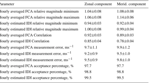
Table 4. Mean and standard deviation of daily relative magnitude minima and maxima, and correlations for hourly estimate IDI and hourly
averaged FCA-large velocities with respect to hourly averaged IDI velocities for 20 August 2000 to 19 September 2003.
Parameter Zonal component Merid. component Hourly averaged FCA relative magnitude minimum 1.04±0.08 1.08±0.08 Hourly averaged FCA relative magnitude maximum 1.06±0.08 1.14±0.06 Hourly estimated IDI relative magnitude minimum 0.94±0.03 0.92±0.04 Hourly estimated IDI relative magnitude maximum 1.00±0.08 0.99±0.04 Hourly averaged FCA Correlation 0.92±0.03 0.89±0.03 Hourly averaged IDI Correlation 0.85±0.04 0.78±0.04 Hourly averaged FCA measurement error, ms−1 9.7±1.1 9.9±1.2 Hourly averaged IDI measurement error, ms−1 9.2±0.9 9.5±1.0 Hourly estimated IDI measurement error, ms−1 9.5±0.9 9.8±1.0 Hourly averaged FCA acceptance percentage, % 97.7 97.7 Hourly averaged IDI acceptance percentage, % 98.8 98.8 Hourly estimated IDI acceptance percentage, % 99.5 99.5
criterion 6 indicates that a turbulent velocity could not be es-timated, a valid velocity is still estimated.
The FCA applies 19 rejection criteria, numbered 1 to 19. The smaller equinoctial FCA acceptance percentages are pri-marily due to rejection of data below 84 km by three rejection criteria:
3: Fading time (half-power half-width of mean autocorre-lation function magnitude) exceeds 8 s.
17: Secondary maxima in the mean autocorrelation func-tion magnitude exceeds 0.5, indicating oscillatory correlafunc-tion functions.
18: Mean autocorrelation function has not passed below 0.5 at last lag of the mean autocorrelation function.
The original motivation for criteria 3, 17 and 18 was to pre-vent the analysis of data indicative of total reflection. This was based on arguments such as those of Hines and Rao (1968) that the FCA would not yield the correct wind veloc-ity if the received signals were due to reflections from regions of layered surfaces perpendicular to the radar beam. The 8-s threshold for criterion 3 has been relaxed from the 6-s thresh-old typically used for wide beam MF radars. This is to allow for larger fading times measured for the BPMF radar, which result from larger diffraction pattern scales due to the rela-tively narrow transmit polar diagram used. A further motiva-tion for criterion 17 is that oscillatory correlamotiva-tion funcmotiva-tions do not fit the assumptions of the FCA, where the spatio-temporal correlation function is assumed to be a monoton-ically decreasing function of spatial and temporal coordi-nates. In early partial reflection observations, further moti-vation for criterion 18 was based on the need to reduce com-putation time by calculating the correlation functions out to a selected maximum time lag. Although criterion 17 has le-gitimate reason to be applied even if total reflection is not oc-curring, it could be argued that criteria 3 and 18 should only be applied above (say) 90 km, if they are indeed intended to
remove data indicative of total reflection. However, another motivation for the use of criteria 3 and 18 is that the accuracy of any estimated correlation parameter (i.e. a correlation or a time lag) is proportional to the fading time, leading to po-tentially large measurement errors in the FCA velocity esti-mates. This is largely supported by our attempts to relax or abandon use of criteria 3 and 18, which has produced signif-icantly more nonsensical than sensible velocity estimates.
The issue of the specular reflection rejection criteria have led to investigation into the use of alternative correlation analyses that avoid the assumptions that spatio-temporal cor-relation functions are assumed to be monotonically decreas-ing functions of spatial and temporal coordinates, and that the spatial and temporal dependence of the spatio-temporal correlation functions are identical. Preliminary investiga-tions (e.g. Holdsworth, 2002) have revealed that the zero-lag cross-correlation slope fitting technique (e.g. Lataitas et al., 1995; Holdsworth, 1995; Holloway et al., 1997) produces sensible velocities for records rejected by FCA. A typical example of equinoctial daytime velocity estimates obtained using the slope fitting technique are shown in Fig. 6. These results show better coverage than the FCA winds, and good agreement with the IDI velocities.
5.3 Hourly velocity comparisons
Table 4 shows the mean daily estimates of the four statisti-cal indicators for the hourly averaged 2-min FCA-large and IDI velocities.This averaging includes outlier rejection and requires a minimum of three velocity estimates per hour to produce an average estimate. The relative magnitudes are in good agreement with the 2-min estimates. The hourly aver-aged correlations are 10% higher than the 2-min estimates, and the IDI measurement errors are smaller than those for FCA-large. We attribute these results to the outlier rejection
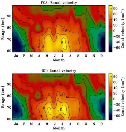
Fig. 7. Annually superposed fortnightly averaged FCA/IDI zonal winds.
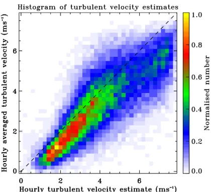
Fig. 9. Scatter plot of hourly averaged 2-min IDI turbulent velocities vs. hourly IDI turbulent velocity estimates over the entire observation
period. The dashed line indicates y=x.
and averaging process precluding spurious 2-min IDI veloc-ities that result from the fewer rejection criteria applied by IDI. The acceptance percentage for both techniques is close to 100%. Thus, although the average acceptance percentage for 2-min FCA velocities is only 56%, an hourly FCA ve-locity estimate for data with average SNR>0 dB can almost always be made.
As described in Sect. 3, IDI is also applied to estimate 1-h wind velocity estimates. Table 4 shows the relative magni-tudes and correlations for the hourly average of the 2-min winds and the hourly estimated winds. Although the correla-tions are high, the hourly estimated winds are approximately 5% larger than the hourly averaged winds. It is not clear to us why this is the case. The measurement errors for the hourly estimates are 3−4% larger. This is in proportion to the rel-ative magnitude, and thus does not indicate that the hourly estimates have larger errors. There is no evidence that one estimate is preferable to the other, although, as discussed in Sect. 5.5, it appears the hourly average of the turbulent ve-locities is preferable to the hourly estimate.
5.4 Long-term velocity comparisons
The annual variation of the FCA and IDI zonal velocities is shown in Fig. 7. These plots represent fortnightly ages, obtained by averaging the 2-min data into hourly aver-ages, which are then used to produce daily averaver-ages, which are, in turn used to produce fortnightly averages. The FCA and IDI winds show excellent agreement, with the IDI again
approximately 10% larger. Of note are the large winds below 70 km in winter, where the IDI winds exceed 85ms−1.
Harmonic analysis of the hourly IDI and FCA estimates have also been performed. Weekly mean, semi-diurnal, di-urnal and 48-h tidal components have been fitted using a 14-day data window every 7 14-days. A superposed plot of the zonal velocity diurnal tide amplitudes for the FCA and IDI data is shown in Fig. 8. The correlation between the FCA and IDI zonal velocity diurnal tidal amplitudes and phases is 0.94 and 0.95, respectively. The corresponding correlations for the meridional velocity (not shown) are 0.96 and 0.91, re-spectively. Smaller, but significant, correlations are seen in comparison of FCA and IDI estimates of other tidal compo-nents (correlations≥0.68). As for the 2-min and fortnightly averaged mean winds, the IDI tidal amplitudes are again ap-proximately 10% larger.
5.5 Turbulent velocities
Figure 9 shows a scatter plot of the hourly average of the 2-min IDI turbulent velocity estimates compared with the hourly IDI turbulent velocity estimates over the entire ob-servation period. Since the distributions of turbulent veloc-ities are not Gaussian, we do not attempt to apply the sta-tistical comparison technique to this data. However, it is clear without applying this technique that the hourly esti-mated turbulent velocities overestimate the hourly average of the 2-min turbulent velocities. As for the FCA turbu-lent velocity estimation (e.g. Holdsworth et al., 2001, and the references therein), IDI turbulence estimation assumes
Fig. 10. Annually superposed fortnightly averaged FCA (top) and IDI (bottom) turbulent velocities.
velocity perturbations in the wind field result solely from tur-bulence. For the 2-min estimates only short period waves (<10 min) will produce velocity perturbations in the radial velocity field, whereas for hourly estimates waves with peri-ods of up to several hours (<5 hours) will produce velocity perturbations in the radial velocity field. We therefore at-tribute the larger hourly estimated turbulent velocities to the effects of gravity waves, and suggest hourly (or larger) tur-bulent velocity estimates (e.g. Roper and Brosnahan, 1997) will be significantly overestimated.
The annual variation of the fortnightly averaged (2-min) FCA and IDI turbulent velocities is shown in Fig. 10. The general trend is an increase of turbulent velocity with height, with maxima below 82 km at the solstices. The IDI turbu-lent velocities show a larger range of values, with smaller minima values and larger maxima values. The larger values at the upper heights are consistent with (as yet unpublished) volume scatter simulations using the radar backscatter model of Holdsworth and Reid (1995), which suggest that the IDI turbulent velocity is overestimated.
6 Interpretation of results in terms of volume scatter predictions
The ESP azimuths are clearly preferentially aligned along the azimuth predicted by volume scatter arguments. This result was also observed using the BPMF radar by Vandepeer and Reid (1995a), albeit over the limited height range of 70 to 84 km. These results differ from the current results in that they were obtained from short-term (4 h) observations, trans-mission using a small antenna array, and using two perpen-dicular receiving antennas arms. The differences in imple-mentation are therefore significant enough to make it dif-ficult for us to conclude why Vandepeer and Reid (1995a) found ESP azimuth agreement with the volume scattering predictions over only a limited range. It could be argued that their use of the “single scatterer” criteria limited their anal-ysis to use only legitimate single scatterers, but in this case there should not have been agreement between the scatterer azimuths and the volume scattering predictions at any az-imuth. Further, it cannot be argued that the difference is due to the larger transmit beam width used in their study, since a larger beamwidth increases the volume of scatterers sampled
at each height, which should increase the number of scatter-ers contributing to each Doppler frequency bin, and thereby increase the agreement with the volume scatter predictions. The results of Fig. 4 further support the suggestion that the ESPs do not represent actual scattering positions. The distri-butions for 90 to 100 km show significant numbers of ESPs at zenith angles outside 12 degrees, despite the transmit power being as low as 30 dB below the main lobe at such zenith angles (e.g. Holdsworth and Reid, 2004), further suggesting that the ESPs do not coincide with the actual scattering posi-tions.
As described in Sect. 5, the FCA true velocities measured by the BPMF radar exhibit the “triangle size effect” (TSE), whereby the true velocity is increasingly underestimated as the spacing decreases. We have used the FCA winds ob-tained using the larger spacing in our analysis to minimise the potential of the triangle size effect to underestimate the FCA winds. Although the volume scatter radar backscatter model simulations of Holdsworth and Reid (1995) showed that the IDI winds exhibit an effect analogous to the TSE for low SNRs, the results of Table 2 suggest that there is no conclusive evidence for such an effect in the current data. Holdsworth and Reid (2004) illustrate that the FCA-large winds are underestimated by around 5% to 10% in com-parison with spatial correlation analysis (SCA) and hybrid Doppler interferometric (HDI), which are both expected to exhibit less bias than FCA winds. The results of Table 3 sug-gests the IDI winds are approximately 8−15% larger than the FCA-large winds, suggesting good agreement with the SCA and HDI winds.
In assessing the applicability of the volume scatter predic-tions we assess two indicators: preferred azimuths, and the ratio of the IDI and FCA velocities. While the results of the former confirm the volume scatter predictions, the results of the latter do not. Ideally, our preference would be to pro-duce plots of the ratio of the IDI to FCA true velocity as a function of turbulent velocity, as shown in Holdsworth and Reid (1995b). However, since the volume scatter predicted IDI to FCA true velocity ratio depends on the wind velocity, turbulent velocity, and ground diffraction pattern scale, we would require a data subset where a large range of turbulent velocities are obtained for limited ranges of velocity and pat-tern scale. Despite collecting three years of data, we have not been able to construct a data subset suitable for produc-ing such a plot. Based on the agreement between the relative magnitudes of IDI, SCA and HDI velocities with respect to FCA-large velocities, we have to conclude that the IDI veloc-ities do not appear to confirm the volume scatter predictions. As described in Sect. 3, one of the motivations behind our application of the Franke et al. (1990) technique was that it shows good agreement with the FCA true velocity. In this regard, the agreement between the FCA and IDI results il-lustrated in this paper is not surprising. One aspect of IDI illustrated by Holdsworth and Reid (1995b) is the sensitiv-ity of the IDI velocities to zenith angle and power thresh-olds. Recent investigations using the same model data set have revealed that the IDI velocity appears to be even more
Table 5. Mean and standard deviation of daily relative magnitude
minima and maxima for IDI without use of radial velocity threshold relative to FCA-large for 19 January 2000 to 3 February 2000.
Parameter Zonal Merid.
component component Relative magnitude minimum 1.32±0.07 1.35±0.07 Relative magnitude maximum 1.36±0.07 1.39±0.07 Correlation 0.85±0.03 0.79±0.05
sensitive to radial velocity thresholds. To illustrate this point, the aforementioned 14-day raw data set has been reanalysed without the use of any radial velocity threshold. The relative magnitudes and correlations of the resulting IDI velocities with respect to the FCA-large velocities are shown in Table 5. These results suggest that the IDI velocity is 35% larger than the FCA-large velocity, and therefore approximately 25% larger than the SCA and HDI velocities, which we be-lieve to be good velocity estimates. We therefore bebe-lieve the good agreement between the FCA and IDI data exhibited by Franke et al. (1990) and in the current study results from the radial velocity threshold used, and that abolishing this threshold results in the IDI velocities being overestimated, in accordance with volume scatter predictions. We note that only two investigators have applied a radial velocity thresh-old for their IDI analysis. Franke et al. (1990) provided no reason for their use of a threshold, while Vandepeer and Reid (1995a) used a threshold on the basis of increasing computa-tional efficiency. There appears to be no obvious theoretical justification for using a radial velocity threshold. A second IDI analysis that does not use a radial velocity threshold has recently been implemented on-line for further investigation.
7 Summary and conclusions
The results of the short-term (2-min) and longer term (hourly, fortnightly averaged, harmonic analysis) comparisons sug-gest that the IDI winds are approximately 10% larger than the FCA-large winds. Apart from this factor, the FCA and IDI velocity estimates show high correlation, and hence very good agreement. However, reanalysis of a 14-day data set without the use of a radial velocity threshold yields IDI winds are that approximately 35% larger than the FCA-large winds, suggesting that the IDI winds are overestimated as predicted by volume scatter arguments.
Regardless of whether the IDI results conform with the volume scatter predictions, this study suggests that the IDI and FCA winds are comparable, and that IDI is a useful tech-nique which has two distinct, significant advantages over the FCA. First, IDI is a significantly simpler technique to ap-ply than FCA, requiring fewer criteria to reject bad data. Second, IDI yields considerably higher 2-min acceptance percentages. However, one disadvantage is that accurate
phase calibration is required. The phase calibration tech-nique used for the BPMF routine observations is described in Holdsworth and Reid (2004). This technique involves pe-riodic determination (e.g. monthly) of phase calibration val-ues, and does not account for complex receiver gain varia-tions that occur over smaller time scales (e.g. diurnal, Van-depeer and Reid, 1995b). It is difficult to assess the ef-fect of complex receiver gain variations on the IDI analy-sis, although this could well be investigated using the radar backscatter model of Holdsworth and Reid (1995b).
One limitation of this study is that the results cannot nec-essarily be considered indicative of those expected for all MF radars, due to the relatively narrow beamwidth used by BPMF radar. We therefore aim to perform a similar study by implementing IDI using a more conventional wide beam MF radar.
Acknowledgements. The Buckland Park MF radar was
sup-ported by Australian Research Council grants A69031462 and A69231890.
Topical Editor U.-P. Hoppe thanks G. Fraser and another referee for their help in evaluating this paper.
References
Adams, G. W., Edwards, D. P., and Brosnahan, J. W.: The imaging Doppler interferometer: Data analysis, Radio Sci., 20 (6), 1481– 1492, 1985.
Adams, G. W., Brosnahan, J. W., Walden, D. C., and Nerney, S. F.: Mesospheric observations using a 2.66 MHz radar as an imaging Doppler interferometer, J. Geophys. Res., 91, 1671–1683, 1986. Briggs, B. H.: The analysis of spaced sensor records by correlation techniques, in: Handbook for MAP, vol. 13, SCOSTEP Secr., Univ. of Ill., Urbana, 166–186, 1984.
Briggs, B. H.: On radar interferometric techniques in the situation of volume scatter, Radio Sci., 30 (1), 109–114, 1995.
Brosnahan, J. W. and Adams, G. W.: The MAPSTAR imaging Doppler interferometer: Description and first results, J. Atmos. Terr. Phys., 55, 203–228, 1993.
Brown, W. O. J., Fraser, G. J., Fukao, S., and Yamamoto, M.: Spaced antenna and interferometric velocity measurements with MF and VHF radars, Radio Sci., 30 (4), 1281–1292, 1995. Charles, K. and Jones, G. O. L.: Mesospheric mean winds and tides
observed by the imaging Doppler interferometer (IDI) at Halley, Antarctica, J. Atmos. Terr. Phys, 61 (5), 351–362, 1999. Franke, P. M., Thorsen, D., Champion, M., Franke, S. J., and
Kudeki, E.: Comparisons of time- and frequency-domain tech-niques for wind velocity estimation using multiple-receiver MF radar data, Geophys. Res. Lett., 17 (12), 2193–2196, 1990. Hines, C. O. and Rao, R. R.: Validity of three-station methods of
determining ionospheric motions, J. Atmos. Terr. Phys., 30, 979– 993, 1968.
Hocking, W. K., Thayaparan, T., and Franke, S. J.: Method for statistical comparison of geophysical data by multiple instru-ments which have differing accuracies, Adv. Space Res., 27 (6– 7), 1089–1098, 2001.
Holdsworth, D. A.: Signal analysis with application to atmospheric radars, Ph.D. Thesis, University of Adelaide, 1995.
Holdsworth, D. A. and Reid, I. M.: A simple model of atmospheric radar backscatter: Description and application to the full
corre-lation analysis of spaced antenna data, Radio Sci., 30 (4), 1263– 1280, 1995a.
Holdsworth, D. A. and Reid, I. M.: Spaced antenna analysis of atmospheric radar backscatter model data, Radio Sci., 30(5), 1417–1433, 1995b.
Holdsworth, D. A. and Reid, I. M.: An investigation of biases in the full correlation analysis technique, Adv. Space Res., 20 (6), 1269–1272, 1997.
Holdsworth, D. A.: An investigation of biases in the full spectral analysis technique, Radio Sci., 32(2), 769–782, 1997.
Holdsworth, D. A.: Influence of instrumental effects upon the full correlation analysis, Radio Sci., 34 (3), 643–656, 1999. Holdsworth, D. A., Vincent, R. A., and Reid, I. M.: Mesospheric
turbulent velocity estimation using the Buckland Park MF radar, Ann. Geophys., 19 (8), 1007–1017, 2001.
Holdsworth, D. A.: Full correlation analysis and specular scatter, ATRAD internal science report # 6, 2002.
Holdsworth, D. A. and Reid, I. M.: The Buckland Park MF radar: Routine observation scheme and velocity comparisons Ann. Geophys., 11, 3815–3828, 2004.
Holloway, C. L., Doviak, R. J., Cohn, S. A., Lataitas, R. J., and Van Baelen, J. S.: Cross correlations and cross spectra for spaced antenna wind profilers. 2: algorithms to estimate wind and tur-bulence, Radio Sci., 32 (3), 967–982, 1997.
Jones, G. O. L., Berkey, F. T., Fish, C. S., Hocking, W. K., and Taylor, M. J.: Validation of imaging Doppler interferometer winds using meteor radar, Geophys. Res. Lett., 30 (14), 1743, doi:10.1029/2003GL017645, 2003.
Jones, G. O. L., Charles, K., and Jarvis, M. J.: First mesospheric observations using an imaging Doppler interferometer adaption of the dynasonde at Halley, Antarctica, Radio Sci., 32 (6), 2109– 2122, 1997.
Lataitas, R. J., Clifford, S. C., and Holloway, C. L.: An alternative method for inferring winds from spaced-antenna radar measure-ments, Radio Sci., 30 (2), 463–467, 1995.
Lesicar, D. and Hocking, W. K.: Studies of the seasonal behavior of the shape of mesospheric scatterers using a 1.98 MHz radar, J. Atmos. Terr. Phys., 54, 295–309, 1992.
Meek, C. E. and Manson, A. H.: Mesospheric motions observed by simultaneous medium-frequency interferometer and spaced an-tenna experiments, J. Geophys. Res., 92 (D5), 5627–5639, 1987. Reid, I. M., Vandepeer, B. G. W., Dillon, S. C., and Fuller, B. M.: The new Adelaide medium frequency Doppler radar, Radio Sci., 30 (4), 1177–1189, 1995.
Roper, R. G. and Brosnahan, J. W.: Imaging Doppler interferometry and the measurement of atmospheric turbulence, Radio Sci., 32 (3), 1137–1148, 1997.
Turek, R. S., Miller, K. L., Roper, R. G., and Brosnahan, J. W.: Mesospheric wind studies during AIDA Act ’89: morphology and comparisons of various techniques, J. Atmos. Terr. Phys., 57 (11), 1321–1343, 1995.
Turek, R. S., Roper, R. G., and Brosnahan, J. W.: Further direct comparisons of incoherent scatter and medium frequency radar winds from AIDA ’89, J. Atmos. Terr. Phys., 60 (3), 337–347, 1998.
Vandepeer, B. G. W. and Reid, I. M.: On the spaced antenna and imaging Doppler interferometer techniques, Radio Sci., 30 (4), 885–901, 1995a.
Vandepeer, B. G. W. and Reid, I. M.: Some preliminary results ob-tained with the new Adelaide MF Doppler radar, Radio Sci., 30 (4), 1191–1203, 1995b.