Emergence of Binocular Disparity Selectivity through Hebbian Learning

HAL Id: hal-02341940

https://hal.archives-ouvertes.fr/hal-02341940

Submitted on 28 Jan 2021

HAL is a multi-disciplinary open access

archive for the deposit and dissemination of

sci-entific research documents, whether they are

pub-lished or not. The documents may come from

teaching and research institutions in France or

abroad, or from public or private research centers.

L’archive ouverte pluridisciplinaire HAL, est

destinée au dépôt et à la diffusion de documents

scientifiques de niveau recherche, publiés ou non,

émanant des établissements d’enseignement et de

recherche français ou étrangers, des laboratoires

publics ou privés.

Emergence of Binocular Disparity Selectivity through

Hebbian Learning

Tushar Chauhan, Timothée Masquelier, Alexandre Montlibert, Benoit R.

Cottereau

To cite this version:

Tushar Chauhan, Timothée Masquelier, Alexandre Montlibert, Benoit R. Cottereau. Emergence of

Binocular Disparity Selectivity through Hebbian Learning. Journal of Neuroscience, Society for

Neu-roscience, 2018, 38 (44), pp.9563–9578. �10.1523/jneurosci.1259-18.2018�. �hal-02341940�

Systems/Circuits

Emergence of Binocular Disparity Selectivity through

Hebbian Learning

X

Tushar Chauhan,

_{Timothe´e Masquelier,}

_{Alexandre Montlibert,}

_and

_X

_{Benoit R. Cottereau}

1_{Centre de Recherche Cerveau et Cognition, Universite´ de Toulouse, 31052 Toulouse, France, and}2_{Centre National de la Recherche Scientifique, 31055} Toulouse, France

Neural selectivity in the early visual cortex strongly reflects the statistics of our environment (

Barlow, 2001

;

Geisler, 2008

). Although this

has been described extensively in literature through various encoding hypotheses (

Barlow and Fo¨ldia´k, 1989

;

Atick and Redlich, 1992

;

Olshausen and Field, 1996

), an explanation as to how the cortex might develop the computational architecture to support these encoding

schemes remains elusive. Here, using the more realistic example of binocular vision as opposed to monocular luminance-field images, we

show how a simple Hebbian coincidence-detector is capable of accounting for the emergence of binocular, disparity selective, receptive

fields. We propose a model based on spike timing-dependent plasticity, which not only converges to realistic single-cell and population

characteristics, but also demonstrates how known biases in natural statistics may influence population encoding and downstream

correlates of behavior. Furthermore, we show that the receptive fields we obtain are closer in structure to electrophysiological data

reported in macaques than those predicted by normative encoding schemes (

Ringach, 2002

). We also demonstrate the robustness of our

model to the input dataset, noise at various processing stages, and internal parameter variation. Together, our modeling results suggest

that Hebbian coincidence detection is an important computational principle and could provide a biologically plausible mechanism for

the emergence of selectivity to natural statistics in the early sensory cortex.

Key words: binocular vision; disparity selectivity; emergence; Hebbian learning; natural statistics; STDP

Introduction

Sensory stimuli are not only the inputs to, but also shape the very

process of, neural computation (

Hebbs, 1949

;

Barlow, 1961

). A

modern, more rigorous extension of this idea is the efficient

cod-ing theory (

Barlow and Fo¨ldia´k, 1989

;

Atick and Redlich, 1992

),

which postulates that the computational aim of early sensory

processing is to use the least possible resources (neurons, energy)

to code the most informative features of the stimulus

(informa-tion efficiency). A direct corollary to the efficient coding

hypoth-esis is that if the inputs signals are coded efficiently, the statistical

consistencies in the stimuli should then be reflected in the

orga-nization and structure of the early cortex (

Geisler, 2008

). The

largest body of work on the efficient coding principle lies within

the visual sensory modality. In the context of vision, a number of

studies have shown that information-theoretic constraints do

in-deed predict localized, oriented, and bandpass representations

akin to those reported in the early visual cortex (

Olshausen and

Field, 1996

). Over the years, several studies have shown how

Received May 18, 2018; revised Sept. 4, 2018; accepted Sept. 5, 2018.

Author contributions: T.C., T.M., and B.R.C. designed research; T.C. and A.M. performed research; T.C. analyzed data; T.C. and B.R.C. wrote the paper.

This research was supported by IDEX Emergence (Grant ANR-11-IDEX-0002-02, BIS-VISION) and Agence Nation-ale de la Recherche Jeunes Chercheuses et Jeunes Chercheurs (Grants ANR-16-CE37-0002-01, 3D3M) awarded to B.R.C.; and the Fondation pour la Recherche Me´dicale (Grant FRM: SPF20170938752) awarded to T.C. We thank Simon J. Thorpe and Lionel Nowak for their comments on the study.

The authors declare no competing financial interests.

Correspondence should be addressed to either Tushar Chauhan or Benoit R. Cottereau, CNRS CerCo (UMR 5549), Pavillon Baudot CHU Purpan, BP 25202, 31052 Toulouse Cedex, France, E-mail:Tushar.Chauhan@cnrs.fror

Benoit.Cottereau@cnrs.fr.

DOI:10.1523/JNEUROSCI.1259-18.2018

Copyright © 2018 the authors 0270-6474/18/389563-16$15.00/0

Significance Statement

Neural selectivity in the early visual cortex is often explained through encoding schemes that postulate that the computational aim

of early sensory processing is to use the least possible resources (neurons, energy) to code the most informative features of the

stimulus (information efficiency). In this article, using stereo images of natural scenes, we demonstrate how a simple Hebbian rule

can lead to the emergence of a disparity-selective neural population that not only shows realistic single-cell and population

tunings, but also demonstrates how known biases in natural statistics may influence population encoding and downstream

correlates of behavior. Our approach allows us to view early neural selectivity, not as an optimization problem, but as an emergent

property driven by biological rules of plasticity.

properties of natural images can not only explain neural

selectiv-ity (

Olshausen and Field, 1996

,

1997

;

Furmanski and Engel, 2000

;

Karklin and Lewicki, 2009

;

Samonds et al., 2012

;

Okazawa et al.,

2015

), but also predict behavior (

Webster and Mollon, 1997

;

Howe and Purves, 2002

;

Geisler, 2008

;

Geisler and Perry, 2009

;

Girshick et al., 2011

;

Cooper and Norcia, 2014

;

Burge and Geisler,

2015

;

Sebastian et al., 2017

).

Nearly all these studies rely on images of natural scenes

ac-quired using a single camera, effectively using a 2-D projection of

a 3-D scene. Although this representation captures the

luminance-field statistics of the scene, it does not fully reflect how visual data

are acquired by the human brain. Humans are binocular and use

two simultaneous retinal projections that enable the sensing of

disparity (differences in retinal projections in the two eyes).

Dis-parity, in turn, can be used to make inferences about the 3-D

structure of the scene, such as calculations of distance, depth,

and surface slant. Despite critical results in the analysis of

luminance-field statistics, only a handful of studies (

Hoyer and

Hyva¨rinen, 2000

;

Burge and Geisler, 2014

;

Hunter and Hibbard,

2015

;

Goncalves and Welchman, 2017

) have attempted to

ana-lyze the relationship between binocular projections of natural

scenes and the properties of binocular neurons in the early visual

system. Furthermore, these studies investigated the relationship

between natural scenes and cortical selectivity in terms of a global

optimization problem that is solved in the adult brain, leading to

cortical structures that encode relevant statistics of the stimuli.

However, the question as to how these encoding schemes might

actually emerge in the early sensory cortex remains, as yet,

unan-swered (

Stanley, 2013

). Here, we show how simple coincidence

detection based on spike timing-dependent plasticity (STDP;

Bi

and Poo, 1998

;

Caporale and Dan, 2008

) could offer a biologically

plausible mechanism for arriving at neural population responses

close to those reported in the early visual system. We endow a

neural network with a Hebbian STDP rule and find that an

un-supervised exposure of this network to natural stereoscopic

stim-uli leads to a converged population that shows single-cell and

population characteristics close to those reported in

electrophys-iological studies (

Anzai et al., 1999

;

Durand et al., 2002

;

Prince et

al., 2002b

;

Sprague et al., 2015

). Moreover, the emergent

recep-tive fields differ from those obtained by optimization-based

methods and are more representative of those reported in the

literature (

Ringach, 2002

). Thus, together, our findings suggest

that the known rules of synaptic plasticity are sufficient to

explain the relationship between biases reported in the early

visual system and the statistics of natural stimuli.

Further-more, they also provide a compelling demonstration of how

simple biological coincidence detection (

Ko¨nig et al., 1996

;

Brette, 2012

;

Masquelier, 2017

) could explain the emergence

of selectivity in early sensory and multimodal neural

popula-tions, both during and after development.

Materials and Methods

Datasets. To simulate binocular retinal input, we chose two datasets—the

Hunter–Hibbard dataset and the KITTI database (available athttp:// www.cvlibs.net/datasets/kitti/). The main results are reported for the Hunter–Hibbard database of stereo images (Hunter and Hibbard, 2015; available at https://github.com/DavidWilliamHunter/Bivis under the Massachusetts Institute of Technology license, which guarantees free us-age and distribution). This database consists of 139 stereo imus-ages of natural scenes relevant to everyday binocular experience, containing ob-jects like vegetables, fruit, stones, shells, flowers, and vegetation. The database was captured using a realistic acquisition geometry close to the configuration of the human visual system while fixating straight ahead

with zero elevation (Fig. 1A). The distance between the two cameras was

close to the human interocular separation (65 mm), and the two cameras were focused at realistic fixation points from 50 cm to several meters away from the cameras. The lenses had a relatively large field of view (20°), enabling them to capture binocular statistics across a sizeable part of the foveal and parafoveal visual field.Figure 1A also shows a red-cyan

anaglyph of one representative scene from the database, whileFigure 1B

shows the images captured by the left and right cameras. Due to the geometry of the cameras, there are subtle differences in the two images (disparity), which provide important information about the 3-D struc-ture of the scene. The mimicking of realistic acquisition geometry is crucial for capturing disparity statistics, which resemble those experi-enced by human observers. For comparison, we also report results using the KITTI database, which uses parallel cameras, a geometry that does not correspond to the human visual system (seeFig. 7and related dis-cussion for more details).

Input sampling. Random locations in the scenes were sampled to

pro-vide inputs to our model. In each simulation, the sampling was restricted to a specific region of interest (ROI). In this article, we present results from the following four main ROIs: foveal (eccentricities⬍3°); periph-eral (eccentricities⬎6°); upper hemifield; and lower hemifield.Figure 1B

shows the foveal ROI shaded in purple. Each sample consisted of two patches corresponding to the two eyes, both centered at the same random retinal coordinates.Figure 1B shows a random sample, with the left patch

outlined in red and the right patch in green. The sizes of the patches varied with the ROI and can be interpreted as the initial dendritic recep-tive field of the V1 neurons, which was subsequently pruned by STDP. In the simulations presented in this article, the foveal patches were 3°⫻ 3°, while the peripheral patches were 6°⫻ 6°. In each simulation, 100,000 input samples were used.

InFigure 3B, we present the results of our model under simulations of

fixations in individuals with strabismic amblyopia. Strabismus is a mis-alignment of the two eyes during fixation and can lead to strabismic amblyopia if left unmanaged during childhood. While strabismic mis-alignment is more accurately represented by an offset of the two camera axes during dataset acquisition, in the absence of this possibility, it was approximated by using a misaligned sampling scheme. The left and right patches of each sample were no longer constrained to be centered at the same retinal coordinates (while still keeping within the ROI). This al-lowed us to simulate retinal activations caused by variable fixations of the amblyopic eye.

Modeling of the retinogeniculate pathway. The computational pipeline

used by the model is shown inFigure 1C. The 100,000 samples were

presented sequentially. The first stage of the model implemented the processing in the retinogeniculate pathway. To simulate the computa-tions performed by the retinal ganglion cells and the lateral geniculate nucleus (LGN), the patches were convolved with ON and OFF center-surround kernels, followed by half-wave rectification. The filters were implemented using difference of Gaussian kernels, which were normal-ized to zero response for uniform inputs, and a response of 1 for the maximally stimulating input. Since the model was to be driven by binoc-ular luminance images, only the magnocellbinoc-ular pathway with achromatic receptive fields, which feed into the dorsal stream (implicated in depth and motion perception), was modeled. The receptive field sizes were chosen to reflect the size of representative LGN center-surround magno-cellular receptive fields: 0.3°/1° (center/surround) for foveal simulations; and 1°/2° (center/surround) for peripheral simulations (Solomon et al., 2002). The activity of each kernel can approximately be interpreted as a retinotopic contrast map of the sample. Four maps were calculated, cor-responding to ON- and OFF-center populations in the left and right monocular pathways. Further thresholding was applied such that, on average, only a small portion (the most active 10%) of the LGN units fired. This activity was converted to relative first-spike latencies through a monotonically decreasing function (a token function, y⫽ 1/x, was chosen), but all monotonically decreasing functions are equivalent (Masquelier and Thorpe, 2007), thereby ensuring that the most active units fired first, while units with lower activity fired later or not at all. Latency-based encoding of stimulus properties has been reported exten-sively in the early visual system (Celebrini et al., 1993;Gawne et al., 1996;

Figure 1. Processing pipeline. A, Acquisition geometry for the Hunter–Hibbard database. The setup mimicked the typical geometry of the human visual system (see more details in the text). This geometry is crucial for capturing realistic disparity statistics from natural scenes. A stereoscopic reconstruction (red-cyan anaglyph) of a sample from the dataset is also shown. B, Input images captured by the left and the right camera for the scene shown in A. The subtle differences in the images (disparity) provide important cues about the 3-D structure of the scene. Depending on the simulation, an ROI in the visual field was identified, and inputs were sampled only within this ROI (foveal ROI illustrated in purple). Each sample consisted of two (Figure legend continues.)

Albrecht et al., 2002;Gollisch and Meister, 2008;Shriki et al., 2012) and allows for fast and efficient networks describing early visual selectivity (Thorpe et al., 2001;Masquelier and Thorpe, 2010;Masquelier, 2012). These trains of first spikes (represented by their latencies) from the ran-dom samples constituted the input to the STDP network.

V1: STDP neural network. The samples were presented to the network

sequentially (Fig. 1C). For each sample, the first spikes from the most

active 10% of LGN neurons were propagated through plastic synapses to a V1 population of 300 integrate-and-fire neurons. Furthermore, a winner-take-all inhibition scheme (Maass, 2000) was implemented such that, if any V1 neuron fired during a certain iteration, it simultaneously prevented other neurons in the population from firing until the next sample was processed. After each iteration, the synaptic weights for the first V1 neuron to fire were updated using an STDP rule, and the mem-brane potentials of the entire population were reset to zero. This scheme leads to a sparse neural population where the probability of any two neurons learning the same feature is greatly reduced. The initial dendritic receptive fields of the neurons were three times the size of the LGN filters (foveal, 3°⫻ 3°; peripheral, 6° ⫻ 6°). At the start, each neuron was fully connected to all LGN afferents within its receptive field through synapses with randomly assigned weights between 0 and 1. The weights were re-stricted between 0 and 1 throughout the simulation. The non-negative values of the weights reflect the fact that thalamic connections to V1 are excitatory in nature (Ferster and Lindstro¨m, 1983;Tanaka, 1985).

The box inFigure 1C shows the processing of the ith sample presented

to the model. Each iteration began with the calculation of the ON and OFF LGN activity maps for the two eyes. This activity was thresholded, converted to spike latencies, and propagated through the network (for more details, see Modeling of the retinogeniculate pathway). The thresh-olding process allowed spikes from the fastest 10% of LGN neurons to propagate through the network. The propagated LGN spikes contributed to an increase in the membrane potential of V1 neurons (excitatory postsynaptic potentials or EPSPs) until one of the V1 membrane poten-tials reached threshold, resulting in a postsynaptic spike and inhibition of all other V1 neurons until the next iteration. The EPSP conducted by the synapse connecting the mth LGN neuron and the nth V1 neuron was taken as the weight of the synaptic connection itself (say wmn). This

allows us to write a simple expression for the membrane potential, En(t),

of the nth V1 neuron at time t within the following iteration:

En共t兲 ⫽

冦

冘

where tmis the spiking time of the mth LGN neuron, H(t) is the

Heaviside step function, and⌰ is the threshold of the V1 neurons (assumed to be a constant for the entire population). The expression

mint兵t兩maxn僆V1En共t兲 ⱖ ⌰其denotes the timing of the first spike in

the V1 layer. The membrane potentials were calculated up to this time

point, after which the winner-take-all inhibition scheme was trig-gered and all membrane potentials were reset to zero.

After the LGN spike propagation, the synaptic weights were updated using an unsupervised multiplicative STDP rule (Gu¨tig et al., 2003). For a synapse connecting a pair of presynaptic and postsynaptic neurons, this rule is classically described as follows:

⌬w ⫽

再

Here, a presynaptic and postsynaptic pair of spikes with a time difference (⌬t) introduces a change in the weight (⌬w) of the synapse, which is given by the product of a temporal filter K [typically, K(⌬t,␶) ⫽ e⫺兩⌬t 兩冫␶_{] and a}

power function of its current weight (w). In our implementation, the efficiency and speed of calculations was greatly increased by making the windowing filter K infinitely wide (equivalent to assuming␶_⫾¡ ⬁, or

K⫽ 1). This, however, does not imply that there was no temporal

win-dowing in the model, as the thresholding at the LGN stage allowed only the fastest 10% of spikes to propagate in each iteration. When a postsyn-aptic spike occurs shortly after a presynpostsyn-aptic spike (⌬t ⬎ 0), there is a strengthening of the synapse, also called long-term potentiation (LTP). Conversely, when the postsynaptic spike occurs before the presynaptic spike (⌬t ⱕ 0), or in the absence of a presynaptic spike, there is a weak-ening of the synapse or a long-term depression (LTD). The LTP and LTD are driven by their respective learning rates␣⫹and␣⫺. The learning rates are non-negative (␣⫾ⱖ 0) and determine the maximum amount of change in synaptic weights when⌬t ¡ ⫾0. The parameters␮⫾僆 [0,1] describe the degree of nonlinearity in the LTP and LTD update rules. In practice, a nonlinearity ensures that the final weights are graded and prevents convergence to bimodal distributions saturated at the upper and lower limits (0 and 1 in our case). Note that, due to the winner-take-all inhibition scheme, the STDP update rule only applied to the afferent synapses of the first V1 neuron that fired. This prevented multiple neu-rons from learning very similar features and was instrumental in intro-ducing sparsity in the limited population of 300 neurons.

For the network used in the present study, the learning rates were fixed with␣⫹⫽ 5 ⫻ 10⫺3and␣⫹/␣⫺⫽ (4/3). The rate ratio␣⫹/␣⫺is crucial to the stability of the network and was chosen based on previous work demonstrating STDP-based visual feature learning (Masquelier and Thorpe, 2007). Our simulations show that the results presented in this article are robust for a large range of this parameter (seeFig. 6). For these values of the learning rate, the threshold of the V1 neurons was fixed through trial and error at⌰ ⫽ 18. This value was left unmodified for all the results presented in this article. Furthermore, we used a high nonlinearity for the LTP process (␮⫹⫽ 0.65) to ensure that we were able to capture fading receptive fields through continuous weights, and we used an almost additive LTD rule (␮⫺⫽ 0.05) to ensure the pruning of continuously depressed synapses. In both LTP and LTD updates, the weights were maintained in the range w僆 [0,1]. It is to be noted that our model was designed to converge to continuous and graded weight distri-butions (as opposed to binary 0/1 weights), and thus the neuronal thresh-old should not be interpreted as the maximal number of full-strength connections allowed per neuron. Finally, the STDP and inhibition rules were active only during the learning phase, and all subsequent testing of the converged populations involved simultaneous spiking of all V1 neu-rons without any synaptic learning.

Analysis of converged receptive fields. The postconvergence receptive

fields of the STDP neurons were approximated by a linear summation of the afferent LGN receptive fields weighted by the converged synaptic weights. The receptive field␰_iof the ith V1 neurone was estimated by the following:

␰i⬇

冘

j僆LGN

wij␺j.

where␺jis the receptive field of the jth LGN afferent, and wijis the weight

of the synapse connecting the jth afferent to the ith V1 neurone. The receptive fields calculated using this method are, in principle, similar to pointwise estimates of the receptive field calculated by electrophysiolo-4

(Figure legend continued.) patches with equal retinal coordinates in the left and the right eye (illustrated in red and green, respectively). All simulations presented in this article were run using N⫽ 100,000 samples each. C, The processing pipeline. The samples were processed sequentially, one per iteration. The processing of the ith sample is shown in the box. First, the ON/OFF processing in the LGN was modeled using difference-of-Gaussian filters in the two eyes—leading to left-ON, left-OFF, right-ON, and right-OFF maps. The activations of the four maps were then converted to first-spike relative latencies using a simple inverse operation (first-spike latencies for only five neurons per LGN map shown in the figure). After thresholding, the earliest 10% of first spikes were allowed to propagate to the V1 layer. The V1 layer consisted of 300 neurons connected to the LGN maps through Hebbian synapses endowed with STDP. A winner-take-all inhibition scheme was also implemented to ensure no more than one neuron fired per iteration. The first spikes from the ith sample were propagated through the synapses, and this was followed by a change in synaptic weights dictated by the STDP algorithm (see text for details about the implemented STDP model). This concluded the processing of the ith sample and was followed by the (i⫹ 1)th_{sample, which was processed in a similar fashion.}

gists. To better characterize the properties of these receptive fields, they were fitted by 2-D Gabor functions. These Gabor functions are given by the following:

G(k,f,␪,␾,x,␴) ⫽ k ⴱ S( f,␪,␾) ⴱ G(x,␴,␪),

where k is a measure of the sensitivity of the Gabor function; S is a 2-D sinusoid propagating with frequency f, and phase␾ in the direction ␪; and G is a 2-D Gaussian envelope centered at x, with size parameter␴, also oriented at an angle␪. A multistart global search algorithm was used to estimate optimal parameters in each eye for each neuron. The process was expedited by using the frequency response of the cell (Fourier am-plitude) to limit the search space of the frequency parameter. For each neuron, the goodness of the Gabor fit was characterized using the maxi-mum of the R2_{goodness-of-fit values in the two eyes, as follows:}

Rmax2 ⫽ max{RLeft2 , RRight2 }.

This ensured that the goodness-of-fit calculations were independent of whether the unit was monocular or binocular.

After the fitting procedure, the Gabor parameters were then used to characterize the structure and symmetry of the receptive field in the dominant eye (defined as the eye with the higher value of the Gabor sensitivity parameter k). This was done by calculating the symmetry-invariant coordinates proposed byRingach (2002). These coordinates [referred to as Ringach coordinates (or RCs) from here on] are derived from the Gabor parameters by the following:

冋

ny

册

⫽

冋

册

f,

where␴xis the spread of the Gaussian envelope along the direction of

sinusoidal propagation,␴yis the Gaussian spread perpendicular to␴x,

and f is the frequency of the sinusoid. While nxis a measure of the number

of lobes in the receptive field, nyreflects the elongation of the receptive

field perpendicular to the sinusoidal carrier. Typical cells reported in cat and monkey have both RCs (nxand ny)⬍0.5 (Ringach, 2002).

The responses of the converged neurons to disparity [disparity tuning curves (DTCs)] were characterized using the following two methodolo-gies: binocular correlation (BC) of the left and right receptive fields; and estimation of responses to random dot stereograms (RDSs). In the BC method, we estimated the DTCs by cross-correlating the receptive fields in the left and the right eye along a given direction. For a given neuron, these DTCs assume that all disparities will elicit responses (i.e., lead to a membrane potential greater than the membrane threshold), and thus represent the theoretical upper limit of the disparity response of the cell. In the RDS method, we estimated the DTCs by calculating the responses of the converged neurons to RDSs at various disparities. The RDS pat-terns used for testing consisted of an equal number of white and black dots on a gray background. The dots were perfectly correlated between the two eyes, with a dot size of⬃15 min visual angles, and a dot density of 0.24 (i.e., 24% of the stimulus was covered by dots, discounting any overlap). The DTC was calculated by averaging the response over a large number of stimulus presentations (N⫽ 10,000 reported here). The re-sponses were quantified by a binocularity interaction index (BII;Ohzawa and Freeman, 1986a;Prince et al., 2002b) given by the following:

BII⫽Rmax⫺ Rmin Rmax⫹ Rmin ,

where Rmaxand Rminare maximum and minimum responses on the RDS

disparity tuning curve. BII values close to zero indicate that the neural response is weakly modulated by disparity, while higher values indicate a sharper tuning to specific disparity values.

The phase and position disparity were estimated by methods com-monly applied in electrophysiological studies— one-dimensional Gabor functions were fitted to the DTCs (for this estimation, we used the BC estimates as they are less subject to noise), and the phase of the sinu-soid and the offset of the Gaussian envelope from zero disparity were taken as estimates of the phase and position disparities, respectively.

Furthermore, the symmetry of the DTCs was evaluated using the symmetry-phase (SP) metric proposed by Read and Cumming (2004). This becomes especially relevant when the shape of the DTC is close to a Gaussian curve, as the phase of the fitted Gabor becomes less reliable. The DTC [say D(␦), where ␦ is the disparity] was first decom-posed into odd (D_⫺) and even (D_⫹) components as follows:

D⫾⫽ 0.5 ⫻ [D(␦) ⫾ D(⫺␦ ⫹ 2␦c)], where␦c⫽

冕

冕

⬁_{兩D(␦)兩 䡠 d␦} is the centroid of D. The SP metric was then

calculated as follows:

SP⫽ Tan⫺1(␰_⫺,␰_⫹),

where␰_⫾is the maximum deviation of D_⫾from zero (including the sign), and Tan⫺1(y, x) is the four-quadrant arctangent function.

Network convergence. The evolution of the synaptic weights with time

was characterized by using a convergence index (CI). If⌬wij(t) is the

change in the weight of the synapse connecting the ith neuron to the jth LGN afferent at time t, the convergence index was defined as follows:

CI共t兲 ⫽ 1

NLGNNV1

冘

冘

兩⌬wij共t兲兩,

where NLGNand NV1are the number of LGN units and the number of the

V1 neurons, respectively. The CI can be interpreted as a measure of the change in the synaptic weight distribution over time. Assuming a statis-tically stable input to a Hebbian network, the number of synapses under-going a change in strength decreases with time. Thus, if our network is driven to convergence, CI should reduce asymptotically with time. To report the convergence for a single unit (say the ith V1 neuron), a mod-ified form of the above index (CIi) was defined as follows:

CIi共t兲 ⫽

1

NLGN

冘

j僆LGN 兩⌬wij共t兲兩.

Robustness analysis. Biological systems show a considerable resilience

to factors such as noise and internal parameter variations (Burge and Jaini, 2017). We tested the robustness of our model using the following three approaches: (1) by introducing timing jitter at both the input and the LGN level; (2) by varying a key internal parameter of our network (the ratio of the LTP rate to the LTD rate); and (3) by comparing results obtained using the Hunter–Hibbard dataset (realistic acquisition geom-etry) to results obtained using a dataset with a nonrealistic acquisition geometry (parallel cameras).

The robustness of the model to noise was tested by adding external (image) and internal (LGN) noise to the system. This simulated timing jitter in the firing latencies from both the retina and the LGN. Gaussian noise with a signal-to-noise ratio (SNR) varying between⫺3 dB (␴noise⫽

2⫻␴signal) and 10 dB (␴noise⫽ 0.1 ⫻␴signal) was used, with␴signalfor a

given image being defined as the variance in pixel grayscale values. The performance of the network at various noise levels was characterized using the following four metrics: the CI; theRmax2 of Gabor fitting; the

population disparity tuning; and the BII. While the CI can be used to evaluate the stability of the converged synaptic connectivity, theRmax2

shows how well the receptive fields can be characterized by Gabor func-tions. Together, the CI andRmax2 characterize the robustness of the

net-work in terms of both the synaptic and the functional convergence. Furthermore, the disparity sensitivity was characterized using the follow-ing two metrics: the population disparity tunfollow-ing calculated usfollow-ing the BC DTC (see Materials and Methods, Analysis of converged receptive fields); and the BII. The population tuning curves give the theoretical encoding capacity of the network, while the BII is a measure of the modulation of network activity as a response to disparity.

The ratio of LTD to LTP rates (␭ ⫽ ␣⫺/␣⫹) is a critical parameter for the stability of the model because it determines the number of pruned synapses after convergence. If the probabilities of LTD and LTP events

are p⫺and p⫹, respectively, the learning rate␥ can be approximated as follows:

␥⬀关p⫹_␣⫹_{⫹ p}⫺_␣⫺_兴.

Given our initial simulation values of the LTD and LTP rates,␣0⫺and␣0⫹,

respectively, we defined␣⫺ ⫽共␣0⫺⁄␤兲and␣⫹ ⫽␤␣0⫹, where the factor

␤ was introduced to ensure that the two rates changed such that the overall learning rate␥ remained stable. The effect of the LTP-to-LTD ratio on the convergence and functional stability of the network was then tested by running simulations for␭ in logarithmic steps from 0.01 to 100 and estimating the CI,Rmax2 , population disparity tuning, and BII

param-eters. This simulated models where the LTD rates were from 1/100 to 100 times the LTP rates.

After testing the robustness of our model to noise and internal param-eter variations, the aim was to test the model on a second dataset. As mentioned earlier, the Hunter–Hibbard dataset used in all our simula-tions was chosen because it has an acquisition geometry close to the human visual system. Thus, for this analysis we chose the KITTI dataset, which was collected using a markedly different acquisition geometry. This dataset uses parallel cameras mounted 54 cm apart, leading to a highly nonecological, zero-vergence geometry. The aim of this analysis was to verify that the main results presented in this article are not specific to the dataset, and that the model is capable of capturing natural disparity statistics while being robust to acquisition geometry. Of course, in this case we did not expect the tunings of the converged neurons to match those reported in human electrophysiology (for more details, seeFig. 7

and related discussion).

Decoding of disparity. The ability of the converged network to encode

disparity was tested through a decoding paradigm. RDS stimuli at 11 equally spaced disparities between⫺1.5° and 1.5° were presented to the converged model, and the first-spike activity of the V1 layer was used to train, and subsequently test, linear and quadratic discriminant classifiers. The inhibition scheme used during the learning phase was turned off, allowing multiple neurons to fire in response to a single stimulus. If we denote V1 activity by the random variable X and disparity by the random variable Y, the probability that the disparity of the stimulus is y, given an observed pattern of V1 activity (say, x) can be written using the Bayes rule as follows:

P共Y ⫽ y兩X ⫽ x兲 ⫽

冘

kP(X⫽ x兩Y ⫽ k)P(Y ⫽ k)

.

In discriminant classifiers, the likelihood term is estimated by, for exam-ple, the following Gaussian density function:

P共X ⫽ x円Y ⫽ y兲 ⫽ 1

冑

where N_V1is the number of V1 neurons, and␮_yand⌺_yare the mean and covariance of the V1 activity for the disparity label y. In linear discrimi-nant classifiers, only one covariance matrix (say,⌺) is assumed to de-scribe the V1 activity for all labels (i.e., ᭙y, 兺y ⫽ 兺). In this case, the

objective function␦_y(x) for the label y can be written as follows:

␦y共x兲 ⴝ logP(Y ⫽ y) ⫺ 1 2␮y T

冘

冘

This leads to discrimination boundaries that are a linear function of V1 activity (this can be verified by setting␦y1⫽␦y2for a given value of x). On

the other hand, quadratic discriminant classifiers allow each group to have a different covariance matrix. In this case, the objective function takes the following form:

␦y共x兲 ⫽ logP(Y ⫽ y) ⫺ 1 2␮yT

冘

冘

冘

冘

leading to boundaries that are quadratic functions of the V1 activity.

We chose RDS stimuli because they do not contain any other infor-mation except disparity. A total of 10,000 stimuli per disparity were used, with a 70/30 training/testing split. Twenty-five-fold cross-validation test-ing was performed to ensure robust results. In this article, we report the detection probability (i.e., the probability of correct identification) at each disparity. It must be noted that here, decoding through classifiers is only an illustrative representation of perceptual responses as it is based on inputs from very early visual processes and ignores important inter-actions such as corticocortical connections and feedback.

Code accessibility. The code for the model is available on ModelDB

(http://modeldb.yale.edu/245409).

Results

In this section, we present the results from simulations (10

iter-ations/simulation) where binocular stimuli from specific ROIs

were presented to our model. In the model, retinal inputs were

filtered through an LGN layer, which was in turn connected to a

V1 layer consisting of 300 integrate-and-fire neurons through

STDP-driven synapses (for details, see Materials and Methods).

The main results are shown for the foveal ROI, while other ROIs

(peripheral, upper hemifield, and lower hemifield) are used to

illustrate retinotopic biases.

Foveal population

Starting from random receptive-fields, the foveally trained

pop-ulation converges to Gabor-like receptive fields found in V1

sim-ple cells (

Movie 1

). This convergence is achieved by a Hebbian

pruning of the initial densely connected dendritic receptive field

of size 3°

⫻ 3°. The mean size of the converged binocular

recep-tive fields when described using a Gabor fit is approximately 1°

(average 1␴ of the Gaussian envelope). Although in the reported

foveal population we started with a 3°

⫻ 3° receptive field,

simu-lations with an initial receptive field size of 6°

⫻ 6° yielded very

similar results. Thus, the pruning process is independent of the

size of the initial dendritic tree and yields converged receptive

fields, which correspond to approximately three times the size of

the central ON/OFF region of the retinal ganglion receptive

fields.

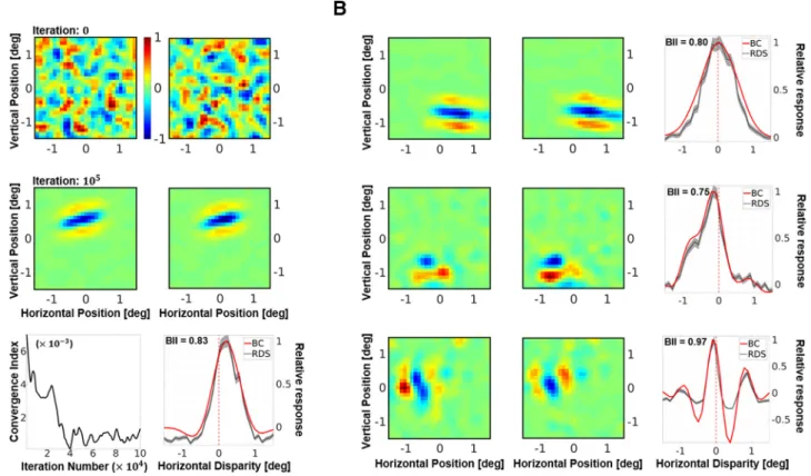
In

Figure 2

A, we present a representative unit from a

popula-tion of 300 V1 neurons. The first row of

Figure 2

A shows the

initial receptive field of the neuron. Since the weights were set to

random values, the resulting receptive field has no specificity in

terms of structure or excitatory/inhibitory subfields. The second

Movie 1. The emergence of receptive fields for neurones shown in Figure 2. The initial receptive fields are randomly connected to the LGN maps. As synapses are strengthened and pruned through learning, we observe the emergence of Gabor-like, binocular receptive fields.

row of the figure shows the receptive field of the same neuron

after STDP learning from 10

_{samples (see also,}

_{Movie 1}

_{). The}

converged receptive field is local, bandpass and oriented. Clear

ON and OFF regions can be observed, and the receptive field

closely resembles classical Gabor-like receptive fields reported for

simple cells (

Hubel and Wiesel, 1962

;

Jones and Palmer, 1987

).

Figure 2

A (bottom left) also shows the CI of the neuron, which

characterizes the stability of its synaptic weights over the learning

period. We find that the fluctuations in the average synaptic

strength decrease over time to a very small value, indicating that

the weight distribution has converged.

In electrophysiology, a neuron with a binocular receptive field

is often characterized in terms of its response to binocular

dispar-ity (

Freeman and Ohzawa, 1992

;

Prince et al., 2002a

,

b

; i.e., its

DTC).

Figure 2

A (bottom right) shows the DTC estimates for the

selected neuron, estimated using both the BC (solid red line) and

the RDS (dotted gray line, with SE marked as a gray envelope)

methods. The DTCs obtained from BC were very similar to those

obtained through RDS stimuli. As the BC DTCs are, in general,

less noisy, they were used to calculate all the disparity results

presented in the article. This neuron shows a selectivity for

posi-tive or uncrossed disparities, indicating that it is more likely to

respond to objects farther away from the observer than fixation.

It also has a high BII (

Ohzawa and Freeman, 1986a

;

Prince et al.,

2002b

) of 0.83, indicating that there is a substantial modulation

of its neuronal activity by binocular disparity (BII values close to

0 indicate no modulation of neuronal response by disparity,

while values close to 1 indicate high sensitivity to disparity

vari-ations). Furthermore,

Figure 2

B shows three other examples of

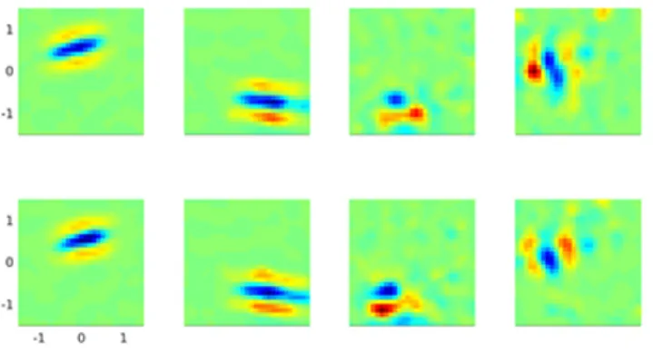
converged receptive fields and the corresponding DTCs (one

neuron per row). The first neuron shows a tuning to zero

dispar-ity (fixation), the second neuron shows a tuning to crossed or

negative disparity (objects closer than the fixation), and the third

neuron shows a tuning curve that is typically attributed to

phase-tuned receptive fields. The receptive fields have a variety of

ori-entations and sizes and closely resemble 2-D Gabor functions.

Receptive field properties

Since most converged receptive fields in the foveal simulation

show a Gabor-like spatial structure, we investigated how well an

ideal Gabor function would fit these receptive fields.

Figure 3

A

shows the goodness-of-fit R

parameter for the left and the right

eye for all 300 neurons in the foveal population, with the color

code corresponding to the value

R

⫽ max {R

, R

}. This

value is maximal of the R

_{parameter across the two eyes, and}

indicates how well the Gabor model fits the receptive field

regard-less of whether it is monocular or binocular. A majority of the

neurons lie along the diagonal in the top right quadrant, showing

an excellent fit in both eyes, with only a few monocular neurons

lying in the top left and bottom right quadrants. It is also

inter-esting to note that, regardless of the degree of fit, the R

_{values for}

the left and the right eye are tightly correlated. This binocular

correlation is nontrivial and cannot be attributed simply to

learn-ing from a stereoscopic dataset, as the interocular correlations in

Figure 2. A, A representative neuron from the simulated population. Receptive fields in the left and the right eye before (first row), and after (second row) presentation of 105_{samples. The}

responses are scaled such that the maximum response is 1. The initial receptive fields are random, while the converged receptive fields show a Gabor-like structure. Bottom left, The CI, which is a measure of the mean change in synaptic strength over time. Bottom right, DTC estimates for horizontal disparity. The neuron shown here is tuned to uncrossed (or positive) disparities. The DTC estimates using two techniques are presented: binocular correlation of the left and right receptive fields (red solid line); and averaging responses to multiple (N⫽104_{) presentations of RDS stimuli}

(gray dotted line). For comparison, both DTCs have been rescaled to have a peak response of 1. The SE for the RDS DTCs is shown as a gray envelope around the average responses. The BII calculated on the raw RDS DTCs is also indicated within the graph. BII is a measure of the sensitivity of the neuronal response to disparity variations, with values close to 0 indicating low sensitivity, and values close to 1 indicating high disparity sensitivity. See Materials and Methods for more details on the calculation of the receptive fields, DTCs, and BII. B, Converged receptive fields and DTCs for neurons showing zero-tuned (first row), tuned near (second row), and phase-modulated (third row) responses to horizontal disparity.

the stimuli compete with intraocular correlations. To

demon-strate this, in

Figure 3

B we show neurons from two simulated

populations: the normal foveal population from

Figure 3

A (red

dots); and a simulated amblyopic population (blue dots). The

neurons in the amblyopic population occupy the top left and

bottom right quadrants (indicating that the neurons are

monoc-ular), as opposed to the binocular neurons from the normal

pop-ulation in the top right quadrant. In the amblyopic poppop-ulation,

the projections in the two eyes were sampled from different foveal

locations within the same image (see Materials and Methods),

thereby mimicking the oculomotor behavior exhibited by

stra-bismic amblyopes. Here, although neurons learn from left and

right image sets with the same wide-field statistics, because of the

lack of local intereye correlations they primarily develop

monoc-ular receptive fields, choosing features from either the left or the

right eye.

Figure 3

C shows the receptive field orientations in the left

and the right eye of binocular neurons in the foveal

popula-tion. Here, we define a binocular unit by using the criterion

min {R

, R

}

ⱖ 0.5 (i.e., both eyes fit the Gabor model with an

R

_{value of at least 0.5). We see that there is a strong}

correspon-dence between the orientation in the two eyes (0° and 180° are

Figure 3. Characterizing a simulated population of 300 foveal V1 neurons. A, The goodness-of-fit R2_{criteria for Gabor fitting in the left and the right eye. Each dot represents a neuron, while the}

filled color indicates the quantityR_max2 _{⫽ max{R} left 2 _{, R}

right

2 _{}, a measure of how well a Gabor function describes the receptive field regardless of whether the neuron is monocular or binocular.} B, Neurons from normal (red dots) and amblyopic (blue dots) populations trained on foveal stimuli (for more details, see Materials and Methods). C, The orientation parameter for Gabors fitted to

the left and the right eye receptive fields. Only neurons with binocular receptive fields defined by the criterionmin{R_left2 _{, R} right

2 _{} ⱖ 0.5are shown. Note that the range of the angles is [0°, 180°],}

with 0° being the same as 180°. D, DTCs for the binocular neurons from C were estimated by the binocular cross-correlation of the receptive fields of the left and right eyes under horizontal displacement. Gabors were fitted to the resulting curves, thereby giving a measure of the position and phase disparity in the receptive fields (Prince et al., 2002a,b). This figure shows the position disparity plotted against the relative phase disparity. It also shows the histograms for the two types of disparities.

equivalent orientations), with a large number of neurons being

oriented along the cardinal directions (i.e., either horizontally or

vertically). Though not shown here, a similar correspondence is

found between the Gabor frequencies in the two eyes (the

fre-quency range is limited between 0.75 and 1.25 cycles/°, due to the

use of fixed LGN receptive field sizes), with an octave bandwidth

of

⬃1.5, a value close to those measured for simple cells with

similar frequency peaks (

De Valois et al., 1982

). Furthermore,

Figure 3

D shows the position and phase encoding of the

horizon-tal disparities as derived by fitting Gabor functions to DTCs

esti-mated by the BC method (for details, see the legend of

Fig. 3

and

Materials and Methods). Both position and phase are found to

code for disparities between

⫺0.5° and 0.5° visual angles (phase

disparities were converted to absolute disparities using the

fre-quency of the fitted Gabor function), with most units coding for

near-zero disparity. Here, we have presented the phase disparity

estimated from the fitted Gabor functions to allow for a better

comparison with previous single-cell studies (

De Valois et al.,

1982

;

Tsao et al., 2003

). However, it has been shown that phases

estimated using Gabor fitting do not accurately characterize the

symmetry of the DTC, especially when the DTC has a

Gaussian-like shape (

Read and Cumming, 2004

). Therefore, to complete

our analysis, we also computed the SP metric (for details, see

Materials and Methods). It revealed that our DTCs were

exclu-sively even symmetric with an SP circular mean

⫽ 2.6° (95%

confidence interval,

⫺2.8° to 8.0°).

In addition to edge-detecting Gabor-like receptive fields,

more compact blob-like neurons have also been reported in cat

and monkey recordings (

Jones and Palmer, 1987

;

Ringach, 2002

).

These receptive fields are not satisfactorily predicted by efficient

approaches such as independent component analysis (ICA) and

sparse coding (

Ringach, 2002

). In

Figure 4

, we present the

distri-bution of RCs for the dominant eye of our converged foveal

population. The n

- and n

-axes approximately code for the

number of lobes and the elongation of the receptive field

perpen-dicular to the periodic function (for more details, see Materials

and Methods). Most of the receptive fields in our converged

pop-ulation lie within 0.5 units on the two axes (

Fig. 4

, blue-shaded

region). These receptive fields are not very elongated and

typi-cally contain 1 -1.5 cycles of the periodic function (

Fig. 4

, cyan

markers show two typical receptive fields of this type). We also

observe blob-like receptive fields (

Fig. 4

, magenta markers),

which display a larger invariance to orientation. In addition, we

show three receptive fields that lie further away from the main

cluster, along the n

-axis with multiple lobes (

Fig. 4

, brown

mark-ers), and along the n

-axis with an elongated receptive field (

Fig.

4

, purple marker). This RC distribution is close to those reported

in cat and monkey recordings (

Jones and Palmer, 1987

;

Ringach,

2002

), while RC distributions found by optimization-based

cod-ing schemes such as ICA and sparse codcod-ing typically tend to lie to

the right of this distribution (

Ringach, 2002

).

Biases in natural statistics and neural populations

The disparity statistics of any natural scene show certain

charac-teristic biases, which are often reflected in the neural encoding in

the early visual pathway. In this section, we investigate whether

such biases are also found in our neural populations.

Figure 5

A

Figure 4. RC distribution for the simulated foveal population (dominant eye). RC is a symmetry-invariant size descriptor for simple-cell receptive fields (for a detailed description, see Materials and Methods). High values along the nx-axis convey large number of lobes in the receptive field, while high values along the ny-axis describe elongated receptive fields. Receptive fields for some

representative neurons are also shown. The pink neurons are examples of blob-like receptive fields, while cyan markers illustrate two to three lobed neurons, which constitute the majority of the converged population. Brown markers show neurons with a higher number of lobes, while the purple marker shows a neuron with an elongated receptive field. Most of the converged neurons lie within the square bounded by 0 and 0.5 along both axes (shaded in blue), something that is also observed in electrophysiological recordings in monkey and cat (Ringach, 2002).

shows a histogram of the horizontal disparity in two simulated

populations of neurons, one trained on inputs from the central

field of vision (eccentricity

ⱕ3°;

Fig. 5

A, purple), and the other on

inputs from the periphery (eccentricity between 6° and 10°;

Fig.

5A

, green). The peripheral population shows a clear broadening

of its horizontal disparity tuning with respect to the central

pop-ulation (Wilcoxon rank-pair test, p

⫽ 0.046). As one traverses

from the fovea to the periphery, the range of encoded horizontal

disparities has indeed been shown to increase, both in V1 (

Du-rand et al., 2007

) and in natural scenes (

Sprague et al., 2015

).

Another statistical bias reported in retinal projections of

nat-ural scenes (

Sprague et al., 2015

) is that horizontal disparities in

the lower hemifield are more likely to be crossed (negative) while

the upper hemifield is more likely to contain uncrossed (positive)

disparities. This bias is not altogether surprising considering that

objects in the lower field of vision are likely to be closer to the

observer than objects in the upper field (

Hibbard and Bouzit,

2005

;

Sprague et al., 2015

). A meta-analysis (

Sprague et al., 2015

)

of 820 V1 neurons from five separate electrophysiological studies

indicates that this bias could also be reflected in the binocular

neurons in the early visual system.

Figure 5

C shows the results of

this meta-analysis, with the probability density for the neurons in

the lower hemifield (in red) showing a bias toward crossed

dis-parities while the upper hemifield (in blue) shows a bias toward

uncrossed disparities. In comparison,

Figure 5

B presents

histo-grams of the horizontal disparity in binocular neurons from two

simulated populations— one trained on samples from the lower

hemifield (red), and the other on the upper hemifield (blue).

Figure 5

(compare B, C) shows that both the range and the peak

tuning of the two simulated populations closely resemble those

reported in electrophysiology. The peaks in

Fig 5

B are at 0.17° for

the upper hemifield and

⫺0.02° for the lower hemifield

(Wil-coxon rank-pair test, p

⫽ 2.15 ⫻ 10

), while the meta-analysis

by

Sprague et al. (2015)

shown in

Fig 5

D reports the values as

0.14° and

⫺0.09°, respectively.

Robustness to internal and external noise

In the results reported so far, the only sources of noise are the

camera sensors used to capture the stereoscopic dataset. To

fur-ther test the robustness of our model, we introduced additive

white Gaussian noise

⬃N(0,␴

) at two stages of the visual

pipeline— external noise in the image, and internal noise in the

LGN layer. The noise was manipulated such that the SNR varied

in steps of

⬃3 dB from ⫺3 dB (␴

⫽ 2 ⫻

␴

) to 10 dB

(␴

⫽ 0.1 ⫻

␴

). Since the noise in these simulations

in-duces timing jitter at the retinal and LGN stages, they are

espe-cially relevant for our model, which relies on first-spike latencies.

In the first and second columns of

Figure 6

, we show the behavior

of the system under internal (in green colors) and external noise

(red colors). The first two panels of

Figure 6

A show the CI of the

network, plotted against the iteration number (training

dura-tion) for the internal and external noise conditions, respectively.

The lightness of the color indicates the level of noise (the darker

the color, the higher the noise). We see that the CI approaches

zero asymptotically in all conditions, indicating that the weights

converge to a stable distribution for all levels of noise. The

corre-sponding panels in

Figure 6

B show the mean

R

, plotted against

the SNR. The mean

R

, as expected, increases with the SNR (the

higher the noise, the less Gabor like the receptive fields). We see

that the receptive fields converge to Gabor-like functions for a

large range of internal and external noise, with the

R

dropping

to

⬍0.5 only at SNR levels ⬍3 dB (␴

ⱖ 0.5 ⫻

␴

). In

Figure 6

C, we show the effect of the two types of noise on

dispar-ity selectivdispar-ity using the population dispardispar-ity tuning and the BII.

While the overall disparity tuning of the converged neural

pop-ulation remains stable in all conditions, we see a marked decrease

in the BII with noise. Since we calculate the population disparity

tuning using BC RDSs (which show the theoretical limit of the

tuning curve), this indicates that, while the receptive fields in the

two eyes converge to similar configurations, their sensitivity

de-creases with an increase in noise.

Overall, these analyses demonstrate that our approach is

ro-bust to a large range of noise-induced timing jitter at the input

and LGN stages. Low-noise conditions produce a synaptically

converged network with Gabor-like, binocular receptive fields.

Under high-noise conditions, the network still converges, albeit

to receptive fields that show a decreased sensitivity to disparity

and are no longer well modeled by Gabor functions.

Robustness to parameter variation

One of the key parameters of a Hebbian STDP model is the ratio

(say,

␭) of the LTD and LTP rates (␣

and

␣

, respectively). This

parameter determines the balance between the weight changes

induced by potentiation and depression, and thus directly

influ-ences the number of pruned synapses after convergence. The

simulations presented in this article use

␭ ⫽ 3/4, a value based on

STDP models previously developed in the team (

Masquelier and

Thorpe, 2007

). In this section, we test the robustness of the model

to variations in this important parameter. The value of

␭ was

varied between 0.01 and 100 in log steps (for the details, see

Figure 5. Retinotopic simulations and population biases in horizontal disparity. A, Histograms and estimated probability density functions for horizontal disparity in two simulated populations of 300 V1 neurons each. The first population was trained on inputs sampled from the fovea (purple), while the second population was trained on inputs from the periphery (green). B, Histogram and probability density estimates of two populations of 300 neurons each, trained on inputs from the upper (blue) and lower (red) hemifields. C, A meta-analysis (Sprague et al., 2015) of results from electrophysiological recordings in monkey V1 neurons (820 neurons in total) by five separate groups. The neurons were split into two groups: neurons with upper hemifield receptive fields are in blue, while those with receptive fields in the lower hemifield are in red.

Materials and Methods). The rightmost column in

Figure 6

shows the results of these simulations.

Figure 6

A shows the CI,

plotted against the iteration number (training period); the purple

colors code for

␣

ⱕ

␣

, and the brown/orange colors code for

␣

_ⱖ

_␣

_{, with the intensity of the color coding for the deviation}

from

␭ ⫽ 1. Once again, the synaptic weights converge for all

values of the parameter, with convergence being quicker for

higher values of

␭.

Figure 6

B shows the mean

R

plotted against

␭. In addition to the modeled values of ␭, here we also show the

value for

␭ ⫽ 3/4, which was used in all simulations in this article.

The model produces Gabor-like receptive fields for a very broad

range of

␭ values (for R

ⱖ 0.5, this range is approximately

between 0.05 and 1). Low values of

␭ (␣

is very low compared

with

␣

) lead to a decrease in performance as the network learns

quickly, and without effective pruning of depressed synapses. For

␣

_ⱖ

_␣

_{, we find that the performance declines (learned}

fea-Figure 6. Robustness analysis. Internal (LGN) and external (Retinal) noise, and parameter (LTD/LTP rate ratio) variation were introduced in the model. The internal (left column) and external (middle column) noises were modeled as additive white Gaussian processes with SNR levels between⫺3 and 10 dB. The ratio of the LTD (␣⫺) and LTP (␣⫹) rates (right column) was varied in logarithmic steps from 10⫺2to 102(i.e.,␣⫺⫽␣⫹/100 to␣⫺⫽␣⫹⫻100).Thisratioisacrucialparameterthatdeterminestherelativecontributionsofsynapticpotentiationanddepression to the overall learning rate. A, CI (see Materials and Methods) for the three types of noise plotted against the number of iterations (training period). For a stable synaptic convergence, the CI should approach zero asymptotically. Internal and external noise are plotted in green and red colors, respectively, with the lightness of the curve coding for the SNR (the darker the curve, the higher the noise). The LTD/LTP rate ratio is plotted in purple colors for␣⫺ⱕ␣⫹and orange/brown colors for␣⫺ⱖ␣⫹. The darker the color, the closer␣⫺is to␣⫹, with black being␣⫺⫽␣⫹. This color coding is used throughout the figure. B, MeanRmax2 . The left and middle plots show the meanRmax2 plotted against the SNR of the internal and external noise respectively. The right plot shows

the meanRmax2 plotted against the␣⫺/␣⫹ratio. An additional dot (outlined in pink) is added to this plot to indicate the value of␣⫺/␣⫹(⫽ 3/4) used for all the simulations presented in the

article (except this figure). C, Population disparity tuning and BII. Each curve in this panel shows the probability density (PD) function estimated over the preferred disparities of a neural population (corresponding to a given condition). Each PD curve is accompanied by an estimate of the mean BII of the neural population (for details, see Materials and Methods), calculated using responses to RDS stimuli. Only neural populations that show a reasonable response to RDS stimuli are shown (otherwise, the BII and PD curves are not meaningful).

tures are more likely to be erased because of the strong pruning),

finally saturating at

␣

ⱖ 6␣

. Furthermore, in

Figure 6

C, we

show how the disparity tuning of the modeled population is

af-fected by a change in

␭. The disparity tuning is stable for 0.05 ⬍

␭ ⬍ 1 (similar to the range that leads to R

ⱖ 0.5), with the

mean BII value increasing as we move from low values of

␭

to-ward

␭ ⫽ 1. For ␣

ⱖ

␣

, the sensitivity of the receptive fields is

very low, and they fail to produce any response to RDS stimuli.

With this analysis, we have shown that our model shows stable

synaptic convergence for all tested values of

␭, and a functional

convergence to Gabor-like binocular receptive fields for a large

range of the parameter (0.05

⬍

␭ ⬍ 1).

Robustness to dataset acquisition geometry

All our simulations (except this section) use the Hunter–Hibbard

database, which was collected using an acquisition geometry

close to the human visual system. The emergent receptive fields

are disparity sensitive and closely resemble those reported in the

early visual system. In this analysis, we prove that this emergence

is not only a property of the dataset, but also of the human-like

acquisition geometry. To do this, the model was tested on

an-other dataset (KITTI; available at

http://www.cvlibs.net/datasets/

kitti/

), which was collected using two widely spaced (54 cm

apart), parallel cameras, which is an acquisition geometry that

does not resemble the human visual system at all (

Fig. 7

A).

Fur-thermore, we present two results from this series of simulations.

Figure 7

B shows the R

value of Gabor fitting in the two eyes

(symbols color coded by

R

) for a population trained on the

foveal region of the KITTI dataset. We observe both monocular

neurons (high R

_{value in one eye, top left or bottom right}

quad-rants) and binocular neurons (high R

_{value in both eyes, top}

right quadrant). In comparison, the converged receptive fields

for the Hunter–Hibbard dataset are mostly binocular (

Fig. 3

A).

This is not surprising as the large intercamera distance (54 cm

compared with 6.5 cm for the Hunter–Hibbard dataset)

com-bined with the parallel geometry results in less overlap in the left

and right images of the KITTI dataset, which further leads to

weaker binocular correlations.

Figure 7

C shows population disparity tunings for two separate

populations trained on the upper (blue) and lower (red)

hemi-fields of the KITTI dataset. As expected, the lower hemifield

pop-ulation is tuned to disparities that are more crossed (negative)

than the upper hemifield population (

Fig. 3

C; see also Biases in

natural statistics and neural populations). For comparison, the

curves for the Hunter–Hibbard dataset (from

Fig. 3

C) are plotted

as dotted lines. The parallel geometry of the cameras in the KITTI

dataset results in predominantly crossed disparities (the fixation

point is at infinity, and hence all disparities are, by definition,

crossed). Thus, while the upper versus lower hemifield bias (see

Biases in natural statistics and neural populations) still emerges

from our model, the population tunings no longer correspond

to those reported in electrophysiological recordings (

Fig. 3

D;

Sprague et al., 2015

).

Decoding disparity through V1 responses

Recently, the effect of natural 3-D statistics on behavior has

been modeled using labeled datasets in conjunction with

task-optimized filters (

Burge and Geisler, 2014

) and feedforward

Figure 7. The KITTI dataset. The model was tested using a second dataset (KITTI; for details, see Materials and Methods), which had a different acquisition geometry. A, Acquisition geometry. The cameras were parallel and separated by 54 cm, a geometry that does not resemble the human visual system. A cyan-red anaglyph reconstruction of a representative scene from the KITTI dataset is also shown. B, Gabor fit. The R2value for the Gabor fit procedure on the left and right receptive fields of the converged neurons, with the color of the symbol coding for theRmax2 (compare toFig.

3A for the Hunter–Hibbard dataset). C, Horizontal disparity tuning. Horizontal disparity tunings for two populations of neurons trained on the upper (blue) and lower (red) hemifields of the KITTI