Modélisation géométrique par primitives

(1)

THÈSE

En vue de l’obtention du

DOCTORAT DE L’UNIVERSITÉ DE TOULOUSE

Délivré par l'Université Toulouse 3 - Paul Sabatier

Cotutelle internationale : Université Victoria

Présentée et soutenue par

Baptiste ANGLES

Le 18 avril 2019

Modélisation géométrique par primitives

Ecole doctorale : EDMITT - Ecole Doctorale Mathématiques, Informatique et

Télécommunications de Toulouse

Spécialité : Informatique et Télécommunications

Unité de recherche :

IRIT : Institut de Recherche en Informatique de Toulouse

Thèse dirigée par

Loïc BARTHE et Brian WYVILL

Jury

M. Andrea TAGLIASACCHI, Examinateur

M. Mathias PAULIN, Examinateur

M. Alec JACOBSON, Examinateur

M. Loïc BARTHE, Co-directeur de thèse

M. Brian WYVILL, Co-directeur de thèse

(2)

GEOMETRIC MODELING WITH PRIMITIVES

by

Baptiste Angles

B.Sc., Universit´

e de Bordeaux, France, 2013

M.Sc., Universit´

e de Toulouse, France, 2015

In Partial Fulfillment of the Requirements

for the Degree of

DOCTOR OF PHILOSOPHY

in the Department of Computer Science

c

Baptiste Angles, 2019 University of Victoria

(3)

GEOMETRIC MODELING WITH PRIMITIVES

by

Baptiste Angles

B.Sc., Universit´e de Bordeaux, France, 2013 M.Sc., Universit´e de Toulouse, France, 2015

Supervisory Committee

Prof. Andrea Tagliasacchi, co-supervisor Department of Computer Science Prof. Lo¨ıc Barthe, co-supervisor Universit´e de Toulouse

Prof. Brian Wyvill

Department of Computer Science Prof. Mathias Paulin

(4)

Abstract

Both man-made or natural objects contain repeated geometric elements that can be interpreted as primitive shapes. Plants, trees, living organisms or even crystals, showcase primitives that repeat themselves. Primitives are also commonly found in man-made environments because architects tend to reuse the same patterns over a building and typically employ simple shapes, such as rectangular windows and doors. During my PhD I studied geometric primitives from three points of view: their composition, simulation and autonomous discovery.

In the first part I present a method to reverse-engineer the function by which some primitives are combined. Our system is based on a composition function template that is represented by a parametric surface. The parametric surface is deformed via a non-rigid alignment of a surface that, once converged, represents the desired operator. This enables the interactive modeling of operators via a simple sketch, solving a major usability gap of composition modeling.

In the second part I introduce the use of a novel primitive for real-time physics simulations. This primitive is suitable to efficiently model volume-preserving deformations of rods but also of more complex structures such as muscles. One of the core advantages of our approach is that our primitive can serve as a unified representation to do collision detection, simulation, and surface skinning.

In the third part I present an unsupervised deep learning framework to learn and detect primitives. In a signal containing a repetition of elements, the method is able to automatically identify the structure of these elements (i.e. primitives) with minimal supervision. In order to train the network that contains a non-differentiable operation, a novel multi-step training process is presented.

(5)

(6)

R´

esum´

e

Les objets naturels ou artificiels contiennent des éléments géométriques répétés pouvant être interprétés comme des formes primitives. Les plantes, les arbres, les organismes vivants ou même les cristaux représentent des primitives qui se répètent. Les primitives se retrouvent aussi couramment dans les environnements créés par l’homme, car les architectes ont tendance à réutiliser les mêmes modèles sur un bâtiment et utilisent généralement des formes simples, telles que des fenêtres et des portes rectangulaires. Au cours de ma thèse, j’ai étudié les primitives géométriques sous trois angles: leur composition, leur simulation et leur découverte autonome.

Dans la première partie, je présente une méthode pour retrouver la fonction par laquelle certaines primitives sont combinées. Notre système est basé sur un modèle de fonction de composition représenté par une surface paramétrique. La surface paramétrique est déformée via un alignement non rigide d’une surface qui, une fois convergée, représente l’opérateur souhaité. Cela permet de modéliser de manière interactive les opérateurs via une simple esquisse, ce qui résout un problème majeur de facilité de modélisation de la composition.

Dans la deuxième partie, je présente l’utilisation d’une nouvelle primitive pour les simulations de physique en temps réel. Cette primitive convient pour modéliser efficacement les déformations des cordes préservant le volume, mais également celles de structures plus complexes telles que les muscles. L’un des principaux avantages de notre approche est que notre primitive peut servir de représentation unifiée pour la détection de collision, la simulation et la déformation de peau. Dans la troisième partie, je présente un cadre d’apprentissage en profondeur non supervisé pour apprendre et détecter les primitives. Dans un signal contenant une répétition d’éléments, le procédé est capable d’identifier automatiquement la structure de ces éléments (c’est-à-dire des primitives) avec une supervision minimale. Afin de former le réseau qui contient une opération non différenciable, un nouveau processus d’apprentissage en plusieurs étapes est présenté.

(7)

(8)

List of Figures

1.1 Examples of recurring primitives in nature . . . 1

1.2 Examples of fractals in nature . . . 2

1.3 Constructive solid geometry . . . 3

1.4 Visualization of convolutional filters . . . 4

2.1 Blending teaser . . . 7

2.2 Simple blend operators . . . 8

2.3 Issues with simple composition functions . . . 9

2.4 Gradient-based operator . . . 10

2.5 Our pipeline to create operators . . . 11

2.6 Design process of sketch-based operators . . . 14

2.7 Sampling of the user sketch . . . 15

2.8 Our operator template . . . 17

2.9 Registration steps of our operator template . . . 20

2.10 Contact operators . . . 22

2.11 Controllability of operators . . . 23

2.12 Interpolation of operator . . . 23

2.13 Tree and leaves composition . . . 25

2.14 Dynamic behavior mimicked by an operator . . . 26

2.15 Contact operators for liquid-glass interaction . . . 26

2.16 Operators simulating droplets interations . . . 27

2.17 Sketch-based composition of a 3D tree . . . 27

2.18 Font design with operators . . . 28

2.19 Droplets on a tree leaf . . . 29

(13)

2.21 Synthesis of operators from previous work . . . 31

3.1 Example of muscle simulation . . . 33

3.2 Structure of a striated muscle . . . 35

3.3 Ziva lion . . . 35

3.4 The parameterization and discretization of a VIPER rod . . . 37

3.5 Static behavior . . . 40

3.6 Dynamic behavior . . . 40

3.7 Real-time soft-body simulation . . . 42

3.8 Elastic band example . . . 44

3.9 Scale-invariant shape matching . . . 46

3.10 Muscle contraction . . . 46

3.11 The mesh-to-VIPER conversion process . . . 49

3.12 Examples of VIPER muscles . . . 49

4.1 An example of MIST architecture . . . 54

4.2 MNIST character synthesis . . . 61

4.3 Two auto-encoding examples learnt from MNIST-hard . . . 62

4.4 Unsupervised inverse rendering of procedural Gabor noise . . . 63

(14)

List of Tables

4.1 Reconstruction errors of MNIST . . . 62 4.2 Detection and classification performance on MNIST-hard . . . 63

(15)

(16)

Acknowledgements

I would like to express my deep gratitude to my advisors Andrea Tagliasacchi and Lo¨ıc Barthe. I am grateful to Andrea Tagliasacchi for the tremendous amount of time he has invested in advising me. I have learnt a lot by working with him and his work ethic has inspired me to give the best of myself during my PhD and forward.

I thank Lo¨ıc Barthe for believing in my potential by offering me the opportunity to pursue a PhD and setting up this jointly supervised program for me.

I am grateful to Brian Wyvill for being my advisor until his retirement. He has been very supportive of my work and has encouraged me to submit to SIGGRAPH Asia, which turned out to be a great piece of advice.

I would also like to thank Kwang Moo Yi for his invaluable guidance on my deep learning work and for being always available to patiently answer the numerous questions I came up with. I have been very fortunate to meet great researchers during and before my PhD. I am particularly grateful to Hugo Gimbert for taking me as an intern in his lab. This experience motivated me to pursue a research path. Mathias Paulin sparked my interest for computer graphics through his captivating lectures and by supervising my master thesis. I would not have published without my co-authors and I would like to thank them for their contributions: Marco Tarini, J.P. Lewis, Javier von der Pahlen, Miles Macklin, Sofien Bouaziz, Julien Valentin, Shahram Izadi, Daniel Rebain, and Thomas Pellegrini. I am grateful to Alec Jacobson for accepting to be the external examiner of my dissertation defense and flying across Canada for the occasion on short notice.

During my PhD, I was fortunate to be surrounded by great labmates and I would like to thank them for the various discussions that helped me with my research: Maurizio Kovacic, Wei Jiang, Kedi Xia, Weiwei Sun, Sri Raghu Malireddi, Abhishake Kumar Bojja, Nicolas Guillemot, and Daniel Rebain.

Finally, my deepest gratitude goes to my father, my mother, my brother, my sister, and my life partner Xiaolu for their support. I thank my parents for suggesting me to study computer science while giving me the freedom to follow my own path. To Xiaolu, thank you for making me happy.

(17)

(18)

Chapter 1 Introduction

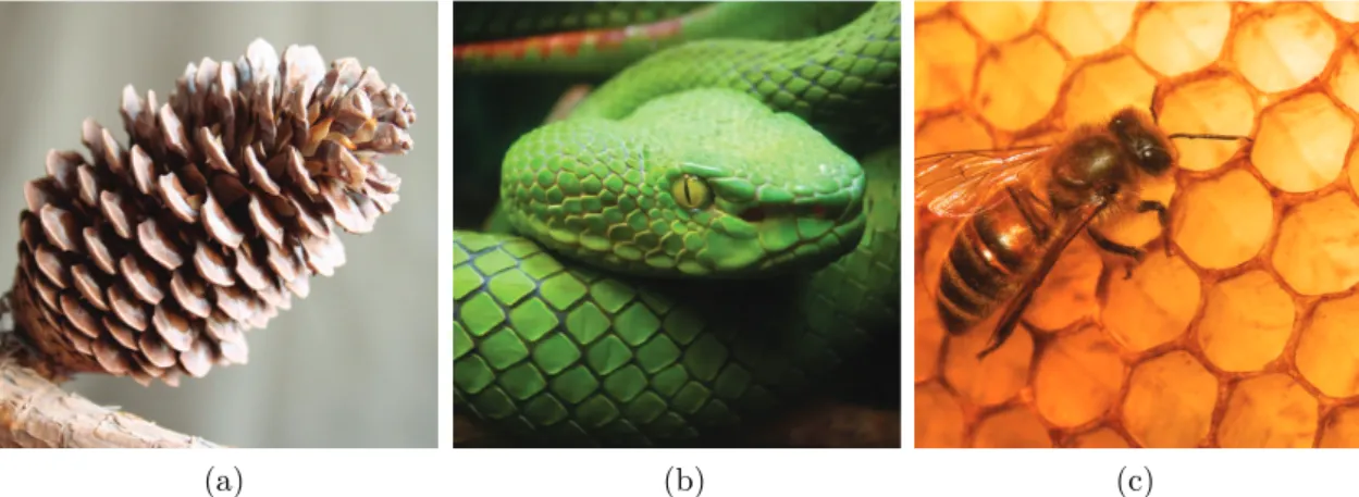
(a) (b) (c)

Figure 1.1: Examples of recurring primitives in nature. (a) A pine cone is composed on dozens of instances of the same primitive shape. (b) The skin of a snake exhibits a repetition of small diamond-shaped scales. (c) Bees build honeycomb structures that are made of a single volumetric primitive. (Sources: pratheep.com, Care SMC, Dominic Heard)

1.1 Motivation

What is a geometric primitive? Looking up the word “primitive” in a dictionary does not give a clear idea. A primitive is defined as something “simple”, “basic”, “elemental”, “unrefined”, or “not derivative”. But the definition that is the most relevant to my research can be found in [Collins, 2004]: “a form from which another is derived”. Primitives are, in fact, defined not by their intrinsic properties but by their role within a larger structure. In this research, we consider geometric primitives to be recurring patterns or shapes that compose an object. Just looking through a window and observing how objects are composed should convince the reader that primitives are very common in our world. But the concept of geometric primitives is also important in computer graphics and computer vision, from geometric modeling to pattern recognition and others. We will then have a closer look at the role of primitives in these three domains: nature, computer graphics and computer vision.

(19)

(a) (b) (c)

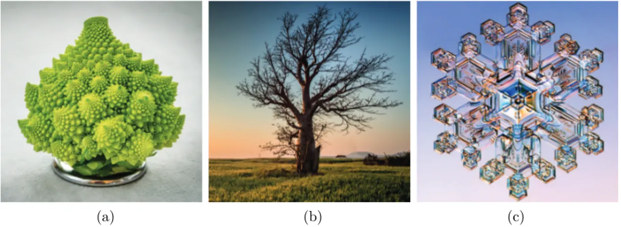
Figure 1.2: Examples of fractals in nature. (a) The Romanesco Broccoli has a fractal-like shape with 4 levels of subdivisions. (b) The branches of a tree split in smaller versions of themselves. (c) A stellar dendrite snowflake that is composed of a central hexagon whose corners spawn another hexagon each. Each secondary hexagon spawns small hexagons at each corner. (Sources: Albrecht Fietz, Sunil Patel, SnowCrystals.com)

Primitives in nature

Repetitions & tessellations. We find plenty of instances of repetitions of elements in nature.

Animals’ skin often exhibit a recurring pattern. This is due to various reasons, involving chemistry [Kondo, 2002] and natural selection [Cott, 1940; Endler, 1980]. For example the skin of a snake is covered by small diamond-shaped scales; see Figure 1.1b. Similarly, many plants’ structures are composed of the same primitives with very little variation stemming from the randomness of the natural process. For instance, pine cones are mainly composed of dozens of instances of a single primitive; see Figure 1.1a. The same thing can be observed for a spiral aloe or many other plants. The leaves of a tree can be seen as randomly varying instances of the same primitive. Bees build hexagon-shaped structures called honeycombs in order to store larvae and honey; see Figure 1.1c. The striking coherence of this structure can be explained by the fact that this shape is a near-optimal solution to the problem of maximizing the cells volume for a given amount of wax [Hales, 2001; Weaire and Phelan, 1994]. One can think of primitives as nature’s response to an optimization problem. Because a shape is optimal for a certain function, it will naturally occur in many places.

Fractals. Many plants are not only structured repetitions of the same primitive but also

self-similar at different scales. Shapes that are infinitely self-self-similar and have a fractal dimension are called fractals [Mandelbrot, 1982]. In nature however, infinite repetition is not attainable but there are many examples of few levels of recursion. For instance the Romanesco Broccoli can roughly be seen as a cone-shaped primitive; see Figure 1.2a. But this cone is filled with smaller cone-shaped elements. And these are themselves filled with similar elements. Trees often exhibit a fractal-like growth where the trunk splits into a few branches, each branch splits into smaller branches, etc; see Figure 1.2b. The fern leaves are composed of leaflets that are themselves composed of subleaflets and look similar to a whole leaf. All snowflakes are different but a lot of them exhibit some form of fractal-like shape. This is the case of the stellar dendrite in Figure 1.2c that is formed of three levels of hexagons.

(20)

Primitives in computer graphics

Efficient rendering. Three-dimensional objects are often represented by a mesh model that

explicitly describes its surface [Botsch et al., 2010]. A mesh is a collection of vertices and polygonal faces. Faces are usually simple geometric primitives such as triangles or quadrilaterals. One of the reasons this representation is popular is that rendering triangles can be done very efficiently using a rasterizer [Akenine-Moller et al., 2018]. Rasterizers are typically implemented to run on GPUs that are designed to execute Single Instruction Multiple Data (SIMD). The OpenGL graphics API only offers to render a few primitives: points, lines, triangles, etc [Shreiner et al., 2013].

Figure 1.3: (left) A CSG composition tree. Primitives are combined pairwise using boolean operations. In the right branch, cylinders are combined by a union operator (∪ symbol). In the left branch, a cube and a sphere are combined by intersection (∩ symbol). At the root the final object is produced by computing the difference between two shapes (− symbol). (right) CAD softwares use CSG operations to model complex objects from simple primitives. (Sources: Zottie, Frank Hull)

Composition modeling. In vector graphics, images are defined by combining together simple

primitives (circles, polygons, curves, etc). These primitives can combined in many ways such as union, difference or intersection. This is exactly the same principle that is applied to 3D in constructive solid geometry (CSG) [Requicha and Voelcker, 1977]; see Figure 1.3. Users can use simple primitives to model complex objects or scenes. L-systems use simple grammar rules to generate realistic shapes such as plants [Prusinkiewicz et al., 1996; Prusinkiewicz and Lindenmayer, 2012] or buildings [Parish and M¨uller, 2001] with simple primitives.

Scene compression. Streaming of 3D data is becoming popular and has applications in scientific

visualization, cultural heritage, digital entertainment, healthcare, robotics, etc. One major challenge is the size of the data that needs to be transferred. Because bandwidth is limited it can cause latency issues which may not be acceptable for some applications, especially for ones where there is a real-time component involved. It is possible to use traditional compression methods but a more efficient way to compress scene data would be to leverage the repetitions and coherency in the geometry of our world. It is possible to represent scenes accurately with simple primitives e.g. man-made environments can often be described by a compact set of recurring elements, such as the windows of a building, or the arrangement of offices and desk in a university. These primitives can be detected or even be learnt and have a much smaller footprint than their corresponding point cloud [Kaiser et al., 2018; Tang et al., 2018a].

(21)

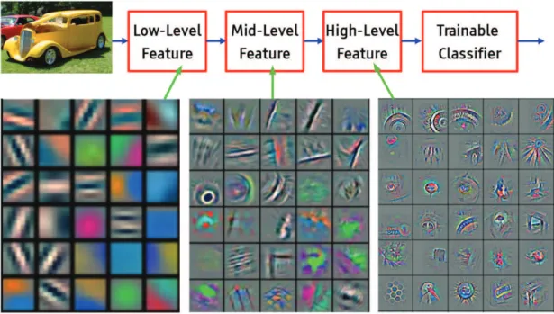
Figure 1.4: Visualization of features maps of a convolutional neural network. (left) The first layers detect edges and intensity contrasts. (middle) The mid-level layers build abstraction upon the previous layers and respond to textures and patterns. (right) The high-level layers identify the present of objects they are trained for in the mid-level feature maps. (Source: [LeCun and Ranzato, 2013])

Physics simulation. Primitives are often used in physics simulation. In the finite element

method (FEM) [Zienkiewicz et al., 1977], complex structures are decomposed into tetrahedra or hexahedra to homogenize the computations. In Lagrangian fluid simulation methods fluids are represented with particles that interact with each other and combine to represent a fluid [Ihmsen et al., 2014]. We can simulate complex objects by discretizing them with simple primitives. This is demonstrated by NVIDIA’s FleX [NVIDIA, 2018], a popular physics simulation library based on position-based dynamics [M¨uller et al., 2007; Macklin et al., 2014]. In this framework, everything including soft bodies, cloth and fluids is represented as collections of particles connected by constraints. Using simple primitives also makes a physics engine simpler because there no need for specialized functions for each object. On GPU it is also more efficient to execute the same function on all the objects. Finally primitives are also used for collision detection [Ericson, 2004]. Testing for collisions between two arbitrary shapes is expensive, so objects are often approximated by simpler primitives [Ritter, 1990; Larsen et al., 2000; Rimon and Boyd, 1992]. For instance the bounding boxes of two objects can be used [O’Rourke, 1985]. It is also common to use bounding volume hierarchies (BVH) [Kaplan, 1985; Kay and Kajiya, 1986] where objects are roughly approximated by one primitive and if the collision test is positive the object’s shape is refined into several primitives, which can themselves contain more levels of hierarchy.

Primitives in computer vision

Pattern recognition. The human visual system is built upon primitives. The cells connected to

(22)

cells of the visual cortex to visual stimuli, Hubel and Wiesel [1959] discovered that these cells build upon several dot detections to detect lines. They also identified complex cells that use groups of

simple cells to detect the movement of lines [Hubel and Wiesel, 1962]. Similarly, one could say

that computer vision uses simple “primitives” to detect complex patterns and shapes [LeCun et al., 2015]. Nowadays convolutional neural networks (CNN) are the state of the art method for object detection tasks [Liu et al., 2018]. CNNs learn convolutional filters to detect patterns in images. These filters detect recurring spatial patterns, i.e. primitives in the image domain, in pictures of objects they are trained to detect. On the first layer, the filters convolving on the input images are in the image domain. Typically the first layers’ filters respond to low-level patterns such as edges and contrast. The ones in the hidden layers respond to primitives in the feature domain. The deeper they are, the higher-level patterns they will be looking for; see Figure 1.4. For instance for face detection, the next layer would be looking to find elements such as noses or eyes. While the last layer should be using looking for a arrangement of eyes, noses, mouth and ears to finally detect a face.

Scene simplification. Primitives can also serve as geometric proxies to simplify a scene and

make it easier to understand. In one of the earliest examples of this, Roberts [1963] attempted to reconstruct a three-dimensional object from a single photograph. His method was based on edge detection which were then converted to simple polygonal primitives to reconstruct the 3D object. This method was only applicable to simple shapes with planar faces but more complex objects can be simplified as aggregates of simple primitives. Fischler and Elschlager [1973] proposed a system where objects like planes are abstracted by a template made of generalized cylinders. This template is not a fixed 3D model and has constrained parameters that vary to match images. Similarly, in [Brooks et al., 1979] objects are decomposed as parts such as eyes and noses that are linked by spatial relations. This serves as a template that can be detected in images. It is a similar idea that is exploited in the recent work on “capsule networks” [Sabour et al., 2017; Hinton et al., 2018].

Body tracking. Body tracking has a wide variety of applications including computer-human

interactions, performance capture, entertainment and telepresence. Thanks to the introduction of low-cost depth sensors on the consumer market, several recent methods propose to tackle the problem from a geometric alignment point of view. These generative techniques require to have a geometric template that can be aligned to the sensor data. One of the problems with these methods is that their template is either inaccurate or inefficient. Typically, implicit templates are used because of their ability to efficiently compute distance queries. But they require a lot of primitives to represent a hand accurately, which makes them inefficient. To solve this, Tkach et al. [2016] represent their hand template with a sphere-mesh, a representation that allows good accuracy with very few primitives.

1.2 Contributions

With the target of modelling a variety of different objects and shapes with simple primitives, we studied how to combine these primitives. Implicit composition operators are very useful for this but they are complex to design. For this reason, in our first project we introduced a method

(23)

to design these operators with simple sketches, which is accessible even to non-technical users. In this first project we often used “tapered capsules”, a primitive that has the ability to model a lot of shapes by varying its few degrees of freedom. This primitive is also very efficient for distance queries and, most importantly, it can preserve its volume while being stretched. For these reasons, in our second project we applied this primitive to real-time simulation of rods, muscles and soft-bodies. In our final project, we perform generative modeling in an “indirect” way, by automatically detecting and learning the primitives that occur repeatedly in a given signal. This is done without any supervision regarding the location or shape of the primitives.

In summary, the contributions of this research are:

1. A method to design composition operators. We introduce a method to design functions that combine implicit primitives via simple sketches. This method enables users to apply composition modeling without requiring any technical knowledge. This is achieved by introducing a template that can represent a wide variety of implicit blending operators. This template is optimized to produce the composition described by a user sketch.

2. A volume-preserving primitive for real-time simulation. We introduce an efficient primitive for volume-preserving deformations. This primitive can be applied to the simulation of rods, muscles and soft-bodies. In order to simulate it in real-time, we extend position-based dynamics by considering scale as a new degree of freedom.

3. A weakly supervised method to learn and detect primitives. We introduce a deep learning framework to automatically identify the structure of repeating elements in a signal. This is made possible by the introduction of a multi-stage process to train through the non-differentiable top-k operation.

Parts of this research have been published in the following papers: 1. Sketch-based Implicit Blending

B. Angles, M. Tarini, B. Wyvill, L. Barthe, A. Tagliasacchi Transactions on Graphics, 2017

2. VIPER: Volume Invariant Position-based Elastic Rods

B. Angles, D. Rebain, M. Macklin, B. Wyvill, L. Barthe, J. P. Lewis, J. Von Der Pahlen, S. Izadi, J. Valentin, S. Bouaziz, A. Tagliasacchi

In Transactions on Graphics (currently under submission to SIGGRAPH 2019) 3. MIST: Multiple Instance Spatial Transformer Network

B. Angles, S. Izadi, A. Tagliasacchi, K. M. Yi In ArXiv (current under submission to CVPR 2019)

The following chapters detail the contributions of this research. This dissertation is organized so that each chapter contains its own necessary background.

(24)

Chapter 2 Composition of Primitives

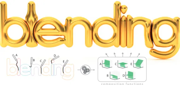
c o m p o s i t i o n f u n c t i o n s A B _C D E A C E B D

Figure 2.1: A user’s 2D sketches (bottom-left) are used to exemplify desired ways in which implicit functions should be composed together. From these, our algorithm automatically derives new custom gradient-based composition operators (bottom-right). These can then be applied to combine any 3D (or 2D) implicit model (top) replicating the user’s intentions, and including effects such as contacts, bulging deformation, or smooth blends.

Abstract

Implicit models can be combined by using composition operators; functions that determine the resulting shape. Recently, gradient-based composition operators have been used to express a variety of behaviours including smooth transitions, sharp edges, contact surfaces, bulging, or any combinations. The problem for designers is that building new operators is a complex task that requires specialized technical knowledge. In this work, we introduce an automatic method for deriving a gradient-based implicit operator from 2D drawings that prototype the intended visual behaviour. To solve this inverse problem, in which a shape defines a function, we introduce a general template for implicit operators. A user’s sketch is interpreted as samples in the 3D operator’s domain. We fit the template to the samples with a non-rigid registration approach. The

(25)

union difference

intersection smooth blend

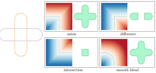
Figure 2.2: Proper design of an implicit composition operator can achieve classical CSG operations such as union, difference, intersection, as well as their smooth variants – i.e. blending.

process works at interactive rates and can accommodate successive refinements by the user. The final result can be applied to 3D surfaces as well as to 2D shapes. Our method is able to replicate the effect of any blending operator presented in the literature, as well as generating new ones such as non-commutative operators. We demonstrate the usability of our method with examples in font-design, collision-response modeling, implicit skinning, and complex shape design.

2.1 Introduction

An implicit representation of a 3D object describes its surface as a set of 3D points on which a scalar function equals a prescribed iso-value [Bloomenthal and Wyvill, 1997]. When modeled or animated, complex objects are defined by assembling their different parts with composition operators, each part being defined by its own scalar function. While the iso-surfaces represent the individual shape of the parts, composition operators control the way they are combined. For instance, the max (min) of two scalar functions produces a union (intersection) operator [Sabin, 1968; Ricci, 1973] which is the basis of Constructive Solid Geometry (CSG) [Requicha and Voelcker, 1977]; see Figure 2.2. The blending operator, in some cases a simple sum of the combined scalar functions [Blinn, 1982], smoothes the sharp transition between parts produced by the union. A core feature of implicit representations is that primitives are combined by simply applying an operator to their respective scalar functions, regardless of their relative positions. This means that no detection or specific treatment for collision is required. This is convenient when the combined primitives are particles of a point-based fluid simulation [Ihmsen et al., 2014], or limbs of a character [Vaillant et al., 2013a].

Several composition operators have been proposed, including controlled blending [Hoffmann and Hopcroft, 1985; Rockwood, 1989; Pasko et al., 1995; Hsu and Lee, 2003], localized blending [Pasko and Adzhiev, 2004], and contact operators that model the contact surface where the combined objects are colliding [Cani, 1993]; see Figure 2.1 for a few examples. Even though these extend the

(26)

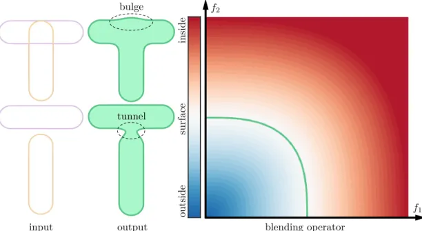
input output blending operator f1 f2 ou ts id e in si d e su rf ac e bulge tunnel

Figure 2.3: A composition operator defined as a function of solely the values of the two input objects presents undesirable bulge and tunnel artifacts.

variety of composition possibilities, they are not commonly used in practice. Some reasons are that meshes are the standard representation for modeling/animation and implicit modeling is not popular on its own, these operators can be computationally intensive, the shape they produce can be unsatisfactory in some cases, and they are often difficult to control by a user.

Recently, gradient-based composition operators [Gourmel et al., 2013] addressed various unsat-isfactory shapes in compositions and computationally expensive operator evaluations. Noting that an implicit surface can approximate a mesh by computing a signed distance field [Macedo et al., 2011], implicit skinning [Vaillant et al., 2014] exploits the automatic contact handling of gradient-based operators on 3D scalar functions for deforming meshes more efficiently when they are animated. This is an example of how implicit modeling/animation tools can be complementary to existing techniques for mesh processing; the current work provides an effective solution to the generalization and intuitive design of free-form gradient-based composition operators.

Composition operators. The scalar functions fa(x), fb(x) : R3 → R of two objects can be

combined with a binary composition operator g : R2_{→ R, and the function f}

c defines the resulting

object as fc(p) = g(fa(p), fb(p)). Even though by suitable choices of composition operators g a

wide variety of transitions can be obtained, many desired behaviors cannot be captured by any choice of the operator [Gourmel et al., 2013]. For example, an operator that produces a smooth blend at a transition will also cause a potentially undesired bulging deformation where two objects overlap, as well as premature bulging before the objects make contact; see Figure 2.3.

The gradient-blend operator. Stemming from these considerations, a richer class of operators

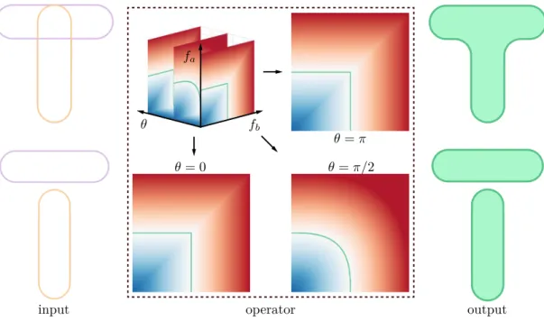
has recently been introduced by Gourmel et al. [2013]. The key idea is to select the operator at each point depending on the value of the angle θ between the local gradient directions of the two scalar functions. More formally, a gradient-based operator g (from now on, simply an operator) is

(27)

θ

fa

fb

θ = 0 θ = π/2

θ = π

input operator output

Figure 2.4: Through inclusion of the gradients angle θ, an operator that is capable of resolving the shortcomings of implicit blending can be designed.

a function (D ⊂ R3_{→ R) that combines two primitives a and b into a new shape c defined as}

fc(p) = g( fa(p), fb(p), θ ) (2.1)

where θ = ∠( ∇fa(p), ∇fb(p) ) (2.2)

∠(v, w) being the angle between vectors v and w. In the rare degenerate cases where this angle is undefined, because the gradient vanishes, θ is 0. The domain of the operator g, i.e. the

operator-space, is D = [0, 1] × [0, 1] × [0, π]

This can be understood as using different composition operators for different values of θ. That is, according to whether the two gradients are in opposite, orthogonal, matching directions, or anything in between. Undesired bulging can be resolved, and pre-contact deformations can be disabled, while in the other cases (intermediate angles) the transition can be kept smooth. Four specific problems of implicit modelling (bulging, locality, absorption, topology) were addressed by defining appropriate instances of g [Gourmel et al., 2013]. The main challenges with gradient-based operators is that designing and fine tuning an operator to obtain some desired effect is a highly technical task, and not possible for non-expert end-users such as 3D artists and modelers. Thus, only predefined and fully parametrized operators can be provided to users and they have to be set in the system by experts.

Contributions. In this research, we address this usability-gap in composition modeling. We

introduce a novel, interactive editing pipeline where the user sketches the desired behavior directly in 2D over one example, and an automatic optimization produces the corresponding operator, transparently to the user. Importantly, the design of an operator and its usage are kept orthogonal: an operator can be applied in any context (2D or 3D) where the same shape or behavior is desired, irrespective of the example where it was designed. Our method can be applied to any shape for

(28)

(a) (b) (c)

input user sketch operator optimization output

D D D

¯s P

Figure 2.5: Given a pair of input primitives (two overlapping circles), the user sketches the desired resulting shape (a contact surface and a bulging effect). (a) The system generates a set of samples in the operator space D. (b) An operator template is fitted to the samples. (c) A dense regular sampling of the operator g is generated. The resulting operator, if applied to the initial pair of primitives, produces the desired behavior and can be applied wherever this effect is desired.

which we can compute a signed distance function. The following contributions were necessary to achieve this result: (1) we introduce a new template to represent operators, which avoids the use of transfer functions such as those proposed in [Gourmel et al., 2013], and is suitable both in the design and in the application phases; (2) we present a way to map user-sketches into samples of operator-space D; (3) we observe that the problem of fitting this template to the samples can be cast as a deformable surface registration problem, and we identify suitable regularizers; (4) we introduce the concept of non-commutative operators, which we show to be useful in certain scenarios, and finally (5) we introduce some novel interesting applications for these operators.

2.2 Related Work

Because of the ease of representing arbitrary and changing topologies, CSG, blended and contact surfaces, implicit modeling has some advantages over traditional surface models [Marschner and Shirley, 2015]. After presenting the previous works on controllable composition operators and an overview of sketch-based implicit modeling, we review some potential applications of our operators.

On freeform operators. Over the years, several operators have been designed to try to fill the

gap between their mathematical formulation and their manipulation by end-users. In aesthetic blends, Pasko and Savchenko [1994] optimize the three parameters of an algebraic blending operator to approximate a user’s sketch. More complex free-form 2D operators have been defined by blending implicit lines [Barthe et al., 2003] or by deforming a blending operator [Barthe et al., 2004]. These operators are subject to all the limitations solved by gradient-based operators and are not compatible with this operator formulation. Rather than focusing on the operator shape, Pasko et al. [2005] and Bernhardt et al. [2010] propose to localize the influence of blending operators on the combined objects by adding an additional 3D scalar function, placed automatically or user-defined. These approaches focus on the definition of where the blending should occur, and no explicit control is performed on the shape of the operator itself. As introduced by Gourmel et al. [2013], the shape of the gradient-based operators are defined by a set of 2D profile curves in cylindrical coordinates. This definition is unintuitive to manipulate and restricted in the variety of shapes it can produce. To achieve better skinning with accurate contact deformations, Vaillant et al. [2014] introduced gradient-based operators discretely computed in a 3D grid, 2D slice by 2D

(29)

slice, by bi-harmonic interpolation of Dirichlet constraints at boundaries and additional constraints on the iso-value. Their specification relies on a lengthy trial and error process, consisting of editing a set of spline curves for a given θ, as well as a trigonometric transfer function to non-linearly interpolate these curves along the θ axis. Furthermore, an interactive exploration is not feasible, as a re-computation of the computationally intensive fairing optimization is necessary on each update. Finally, their operator construction is tailored to a small set of effects useful in the targeted context (symmetric contacts and bulges), whereas our operators are generic. In our work, we enable the specification of freeform gradient-based operators at interactive rates through the use of 2D annotations, which directly describe the intended user-defined behavior.

Sketch based implicit systems. Sketches have long been recognized as a powerful tool for

modeling [Igarashi et al., 1999]. Sketch-based implicit systems added the ability to do blending and CSG with volume models in work such as [Singh and Fiume, 1998; de Ara´ujo and Jorge, 2003; Alexe et al., 2005; Tai et al., 2004], and there have been several examples, including the popular ShapeShop by Schmidt et al. [2005]. [Singh and Fiume, 1998] shares with us the idea that the final surface shape is modelled by a 3D curve. Closer to our proposal, Karpenko et al. [2002] built models using an implicit representation based on Radial Basis Functions. Their system used the input stroke to edit a mesh, which would in turn change the implicit representation. This implicitization approach changes the field locally according to the user’s edit. In the above approaches, sketches define the shape in one particular modeling instance. The input sketch in our system defines an operator, which is not tied to the context where it is defined, but can be applied wherever the user desires.

2.2.1 Applications

This work impacts several application domains, offering interesting contributions in each of them.

Character skinning. In the context of character skeleton-driven animations, composition

operators have been used to achieve more realistic procedural skin distortions [Vaillant et al., 2013a, 2014]. This is also a motivation for our work. With respect to these applications, our approach offers the ability for the designer to intuitively sketch the exact intended deformation (e.g. skin bulging) in one instance, and produce an operator which will reproduce that deformation in real time. This approach is analogous to example-based deformation schemes (see [Jacobson et al., 2014b] or [Shi et al., 2008]), but in our case, the exemplar sketch can be drawn in 2D, and the extracted operator can be directly applied to any other joint.

Font design. One potential application of our method is to assist font-design, where glyphs for

each letter are the result of composition operators in 2D from a pre-defined skeleton; similarly to [Suveeranont and Igarashi, 2010]. The literature on font design is large, and covers many problems which are not addressed here, including automatic construction of the skeletons, or a consistent cross-parameterization for all glyphs, or even a generative manifold of all possible fonts; see [Campbell and Kautz, 2014]. In pipelines where the skeletons of each glyph becomes available, our method offers the ability to control the shape of one glyph (e.g. serifs and joints), and apply it consistently to the entire type-face.

(30)

Botanical modeling. In the context of procedural synthesis of botanical models (both realistic

and stylized), implicit models have been recognized early as suitable solution, due to their natural ability to recreate smoothly blending branching structures [Bloomenthal, 1995; Hart and Baker, 1996; Galbraith et al., 2004]. Using our tool, a user can simply trace the required shape to mimic the geometry of these features, and incorporate this effect into the operator.

2.3 Method Overview

A visual outline of our framework is illustrated in Figure 2.5. Our design process begins with the user placing two exemplar implicit primitives in a 2D sketch. The user then annotates the desired blending behavior by sketching a curve. Given this input, an automatic system derives an operator

g by solving an inverse optimization problem; see Section 2.6. The resulting operator can then be

used both to combine implicit curves in 2D and to combine surfaces in 3D. This observation is crucial, as it allows the user to simply work in 2D to produce operators for 3D modelling. This is even more relevant for the design of contact surfaces, which would otherwise be difficult to edit (or even just to visualize) in 3D, due to self-occlusions.

Feedback loop. In many cases, a single set of user sketches are sufficient to fully determine the

operator g that produces the desired result; see Figure 2.5. For more complex cases, an iterative feedback loop can be used to refine the operator and at the same time observe its effect; see Figure 2.6. First, an operator g0 is constructed from an initial sketch and automatically applied

to the exemplar primitives. The resulting 2D drawing provides feedback to the user. The user can then add new sketches, and a new operator is produced from the union of all sketches. This is repeated until a satisfactory shape is returned to the user, limited only by the expressiveness of the gradient-based approach; see Section 2.7. In practice, we found we needed no more than three iterations. For the feedback loop to be interactive, we need to ensure that our algorithms are computationally efficient for the optimization of the operator and for its application.

2.4 Background and preliminaries

An implicit model (surface in 3D, or contour, in 2D) is defined by a scalar field-function f , as the set of the points where f assumes a given iso-value. Following the convention from Bloomenthal and Wyvill [1997], we define the surface as S = {x ∈ Rn_{|f (x) = 0.5} which bounds an interior}

where f (x) > 0.5. The field-functions of the primitives are, in turn, defined by their skeleton. For example, a sphere is generated by a point skeleton, and a capsule (a cylinder with hemispherical caps) by a line-segment skeleton. Any other shape can be used; see Figure 2.13,2.18 for some examples.

Support and continuity. The field has a value which decreases with the distance from the

skeleton, according to a given falloff function; see [Marschner and Shirley, 2015]. The area where the field function has values |f (x) − 0.5| < 0.5 is denoted the support of the implicit object. Outside its support, the field function equals zero and the primitive has no influence on the composition operations. The support is compact, i.e. bounded; see Figure 2.7.

(31)

1

2

3

input+sketches kernel+samples feedback

final operator

Figure 2.6: Operator design feedback loop: because our pipeline (Fig. 2.5) has interactive response times, our system allows progressive refinement of the operator though successive strokes. Undesired blending artifacts (right) are corrected until a final operator is constructed which is capable of reproducing the desired behavior.

(32)

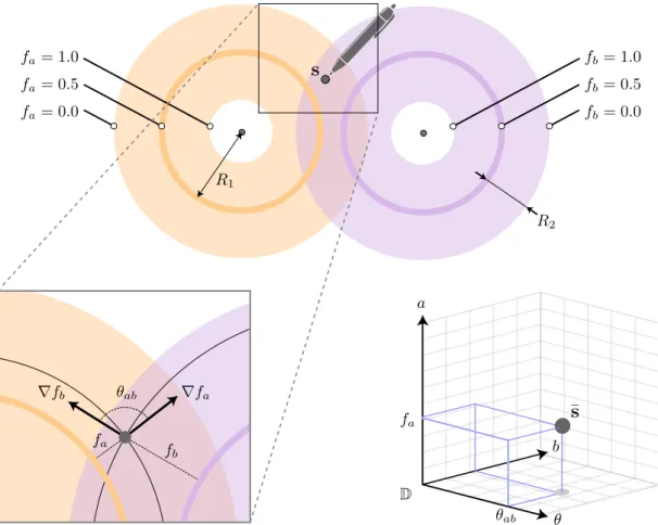
s

fa = 0.0 fa = 0.5 fa = 1.0 fb= 0.0 fb= 0.5 fb= 1.0 R1 R2 ∇fa ∇fb fb fa θab D θ a b fa θab

¯

s

Figure 2.7: Top: a sample s is drawn in the intersection of the supports of the two primitives (bold colored lines) generated by the skeletons (black dots). Lower-left: a zoom-in around s: the gradients of the two field functions fa and fb form an angle θ. Lower-right, the corresponding

sample ¯s in the operator’s domain D (see Eq. 2.5).

A central concern in implicit operator design is to ensure smooth blends and avoid normal discontinuities at the boundaries of the support. To this end, where functions such as min or max are used for g [Barthe et al., 2003], filter fall-off functions are required to be at least C1_{. In our}

approach, where we fully control the composition function g, this requirement can be completely dropped. Instead, we rely on functions g with built-in smoothness, by defining appropriate value and derivative constraints at the boundaries of its domain D; see Section 2.6.3. This observation allows us to use any monotonic C0_{fall-off function for our primitives. In our examples we opt for}

a simple linear function controlled by two intuitive parameters: R1, the iso-value of the implicit

model, and R2, the thickness of the support; R1is mapped to 1/2 and R1+ R2to 0 (see Figure 2.7,

top). In the example of Figure 2.13, the curly branches are obtained by linearly interpolating two values of R1 along the skeletal curve of the branch.

Intersection and difference. In this research, we concentrate on union composition operators

g, which fuse two primitives into one in some prescribed manner, i.e. g always returns 1 when either of the first two parameters is 1, and 0 when both are 0. Generalization to intersections and

(33)

differences is straightforward using the same g:

gintersection(a, b, θ) = 1 − g(1 − a, 1 − b, θ) (2.3)

gdifference(a, b, θ) = 1 − g(1 − a, b, θ) (2.4)

Implicit composition. The creation of complex geometry requires the composition of more

than just two input functions. Following the ideas introduced by Wyvill et al. [1999], we employ different binary operators at each node of a tree, with primitive shapes at its leaves. For example, see Figure 2.1 where different operators are used in cascade.

2.5 Capturing user inputs

In our system, a pair of 2D primitives are arranged freely by the user; see Figure 2.6 for an example. The linear field functions fa and fb of the two primitives are expressed in closed form, and to the

user, the two primitives are visualized as closed poly-lines. In Figure 2.7, we also visualize the supports Sa and Sb of the two shapes. By construction, the target operator can only determine

the resulting shape in the area Sa∩ Sb, therefore user input strokes are restricted to be inside this

area with a stencil mask. The user draws the desired shape of the resulting surface over the input primitives, with one or multiple sketches. For most experiments we employ parametric curves, but any drawing method such as the strokes in Figure 2.20c, can be used. As described below, this is possible as only a sampling of the sketches is required to derive an operator.

Sampling user input. From the user’s sketch, we extract a set of n samples {s1, . . . sN}. Each

sample sn∈ R2represents a position that the user expects the result/output surface to cross. As

illustrated in Figure 2.7, for each sample sn we define a corresponding sample ¯sn in the operator

domain D: ¯sn=      an bn θn      =      fa(sn) fb(sn) ∠( ∇fa(sn) , ∇fb(sn) )      (2.5)

Computations of ¯sn from sn are conveniently fast because functions fa and fb are available

in closed form. Their gradient is either available in closed form or approximated by finite differences. The regressed operator g evaluated at ¯sn should return the value (0.5), or in other

words g(¯sn) = 0.5. Hence, after optimization, the designed blending operator kernel g should

interpolate each sample ¯sn.

Sketches over 3D rendering. As a variation, sketches can be drawn over a 3D rendering of the

implicit surfaces, seen from arbitrary viewing angle; e.g. see Fig. 2.17. In our prototype, the sketch is in this case assumed to lie on an plane parallel to the image at a predefined depth. In situations where the gradients of the primitives are not co-planar, there is no ideal plane to sketch on and results could be unintuitive. In this case, it is often better for the user to sketch on a simpler configuration of primitives and to then apply the operator to the original scene. Our framework requires no further adaptation to deal with this case. A more advanced interface could identify depth automatically, for instance by projecting the first point of the sketch on the shape, similarly

(34)

a

b

θ

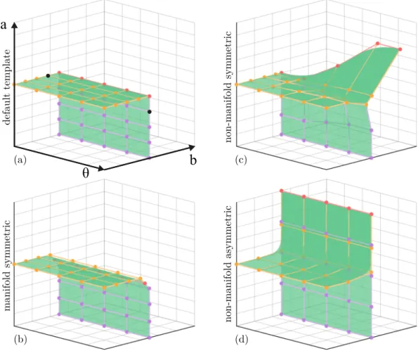
(a) (b) (c) (d) d ef au lt te m p lat e m an if ol d sy m m et ri c n on -m an if ol d sy m m et ri c n on -m an if ol d as y m m et ri c

Figure 2.8: Our template is a surface P is made of two bi-quadratic patches, depicted with orange and violet control points – red ones are shared, creating a seam at the junction. This template is able to represent a variety of useful composition operators; see Section 2.6.2.

to the sketch-based modeling interface proposed by Bernhardt et al. [2008].

2.6 Fitting the composition operator

The blending operator requires a 3D function g to be defined over its entire space D, however samples collected from user’s strokes only define the behavior of g in a small subset of D. On the other hand, many characteristics of the function g are known a-priori, such as its general shape (Sec. 2.6.1), its continuity requirements (Sec. 2.6.2) and the values on the boundaries of D (Sec. 2.6.3). We approach this reconstruction problem in two steps: first, we identify the set of 0.5 values of g, as a parametric surface P embedded in D, which is fitted to the samples (Sec. 2.6.4); we then compute a 3D lattice covering the domain of g by propagating the iso-values in P (Sec. 2.6.5). The final operator is then evaluated by tri-linear interpolation of the lattice values.

(35)

2.6.1 The operator template

In previous work [Gourmel et al., 2013; Vaillant et al., 2013a, 2014], g(a, b, θ) is formulated as a collection of two dimensional functions for a few particular values of θ, each independently defined as a curve defining the portions of the domain where g evaluates to (0.5). These cases can be interpreted as axis aligned slices of the domain D. In our work, we conveniently represent the operator g as one surface P embedded in D representing its (0.5) iso-value; see Figure 2.5b. This approach allows us to define a template for the surface P , designed to represent a wide class of useful operators: sharp unions (see Figure 2.8a), smooth blends (see Figure 2.8b), articulated contact (see Figure 2.8c) and asymmetric contact (see Figure 2.8d) amongst many others; see Figure 2.21.

Parametric representation. Our template for P is a surface made by a pair of third-order

B-Spline patches, each with I × J control points, joined at their boundary and arranged as in Figure 2.8a. The surface P is fully determined by the positions of the control points pa

i,jand pbi,jin

D. We found I=J=5, for a total 45 distinct control points, to provide the necessary expressiveness while avoiding excessive redundancy. The continuity of P at the junction is enforced by imposing ∀i ∈ [1..I] : pa

i,J = pbi,J, while other boundary and regularization constraints will be discussed later.

2.6.2 Template expressiveness

A fundamental characteristic of our operator template lies in its expressiveness. In particular, in Figure 2.21 we illustrate how, to the best of our knowledge, all results obtained by any composition

operators which have been proposed in the literature can be expressed by our template. We now

detail how several operators can be realized by properly deforming our template.

Sharp creases: if a sharp crease is desired in the transition between the two operand surfaces

(e.g. with union) then g needs to break C1_{continuity, and consequently P must have a normal}

discontinuity. In our template, this discontinuity is easily accommodated by construction at the junctions between the two splines.

Smooth blends: if g is required to generate surfaces without any sharp creases in the transition

between the two operand surfaces, it needs to be C1continuous, and consequently, surface P must be smooth, including at the junction between splines. This can be easily obtained by aligning the points{pa

i,J −1, p a i,J= p b i,J, p b i,J −1}.

Contact surfaces: another important feature of operators is the ability to produce contact

surfaces at the transitions between the two primitives [Cani, 1993; Vaillant et al., 2014]; see

Figure 2.21efg. Our template can easily reproduce this situation by making the two patches partially coincide, thus realizing a non-manifold operator.

Symmetry: many existing composition operators g are commutative in their first two parameters,

which in our setup makes surfaces P symmetric with respect to the a = b plane in D. Given

φ : D → D is the planar mirroring transformation φ(x, y, z) = (y, x, z), this can be easily

obtained by enforcing pa

i,j= φ(pbi,j). Clearly, non-commutative operators, such as those in

(36)

In summary, our template can recreate each of the features above. If required, our system allows users to explicitly enforce these conditions; however, it is not strictly necessary to do so, as surface

P will naturally conform to these conditions whenever they are suggested by the user data as a

result of the fitting process. This observation can aid the design of user interfaces based on our method.

2.6.3 Boundary conditions

When fa(p) = 0, the point p is outside the (compact) support of fa, and hence beyond its range

of influence, so fc should exactly reproduce the values of fb(p) to ensure C0 continuity. Analogous

considerations apply to the fb(p) = 0, fa(p) = 1 and fb(p) = 1 boundary planes of D, leading to

the constraints:

∀θ, ∀a : g(a, 0, θ) = a and g(a, 1, θ) = 1

∀θ, ∀b : g(0, b, θ) = b and g(1, b, θ) = 1 (2.6) Further, to achieve (normal) shading smoothness at the boundaries of the supports, we must enforce C1_{continuity of the blending operation by vanishing the derivatives:}

∀θ, ∀a : ∂g_∂b(a, 0, θ) = 0, ∀θ, ∀b : ∂g_∂a(0, b, θ) = 0 (2.7)

As θ represents the unsigned angle between the two gradient vectors, the function g is implicitly mirrored at both ends [0, π] of its third parameter. Therefore, to achieve C1_{continuity we also}

impose:

∀a, ∀b : ∂g

∂a(a, b, 0) = 0 ∀a, ∀b : ∂g

∂b(a, b, π) = 0 (2.8)

The constraints above translate into Dirichlet and Neumann boundary conditions for surface P , which can be conveniently expressed in terms of linear hard constraints on its control points. To enforce Equation 2.6, the control points on opposite ends of P are constrained to lie on the two line segments at the boundary of D: (0.5, 0, θ) and (0, 0.5, θ). To enforce Equation 2.7 and Equation 2.8, the control points neighboring the boundaries of P must be constrained to be vertically/horizontally aligned to the boundary control points.

2.6.4 Surface registration

In this phase, we fit the template parametric surface P to the collected samples ¯si. P maps

each point uv = (u, v) of its 2D parametric space into a position P (uv) ∈ D, as determined by the control points {pk

i,j}. We start with an initial guess, which corresponds to a union operator:

a surface P where the two B-spline patches are simply planar and reciprocally orthogonal; see Figure 2.8a. We then non-rigidly register the template onto the samples following the approach in [Bouaziz et al., 2016]; see Figure 2.9. This optimization consists of the alternation of two

(37)

t= 1 t= 3 t= 4 t= 6 t= 9

Figure 2.9: We illustrate the sketches in operator space, and a few iterations of the operator registration optimization in Equation 2.10. The manifold surface folds onto itself to be able to reproduce a non-manifold configuration. At the same time, the way we enforce the symmetry constraint helps the optimization to avoid undesirable self-intersections. In this example, the optimization converged after 9 (two-steps) iterations; none of our experiemnts required more than 20.

optimization steps:

local: arg min

(uvn)

kP (uvn) − ¯snk2, ∀¯sn (2.9)

global: arg min

{pk i,j}

Ematch({pk_i,j}, {uvn}) + Epriors({pk_i,j}) (2.10)

That is, our local-global ICP optimization first computes closest-point projections, and then it globally modifies the surface control points, resulting in a non-rigid deformation of our surface. For sample points corresponding to a contact surface, both sides of the template must be separately fitted to these. These sample points could be labeled automatically but we let the user provide this information. To efficiently implement the local step, we first triangulate P (we employ a resolution of 40 × 40), and use a regular volumetric grid to accelerate closest-point queries from ¯sn to the triangles. We also constrain each of the I rows of control points to lie at a constant

equally spaced θ values. The global step is implemented as one Least Squares minimization, as both energy terms are quadratic in the variables; Ematch represents the data-to-model error, while

Eprior accounts for shape-priors as well as optimization regularization. Further implementation

details are available in our publicly released source code.

Matching term. The data-to-model error is computed as the averaged squared distances of

samples from the tangent planes of their projections onto P :

Ematch = 1 N X n [nn· (¯sn− P (uvn))]2 (2.11)

where nnis the normal at P (uvn). This point-to-plane metric leads to better convergence compared

to point-to-point errors. The term is a quadratic function of the variables, because P (uvn) and

nn are both constants in the global step.

Priors. The prior energy includes several terms weighted by parameters. These terms enforce:

operator fairness, potential contact constraints, and regularization of the optimization:

(38)

Fairness prior. We penalize oscillations in the surface with a bi-harmonic energy defined on the control points pk i,j: Efair = X i,j k∆uvpki,jk2 (2.13)

where ∆uv represents the 2D Laplacian operator defined in the uv domain, adapted to have

control vertices stored in matrix form pk

i,j. This regularizer has multiple advantages: (1) in

under-sampled areas it ensures a smooth interpolation, (2) it prevents over-fitting and, (3) as the sketches only provide a sparse sampling in D, it regularizes our optimization ensuring the problem remains well-conditioned. Additionally, these fairness energies are known to penalize surface fold-overs [Botsch and Kobbelt, 2004]. Following [Li et al., 2008], we start by a strong enforcement of fairness to avoid local minima, and progressively relax this constraint to allow the surface to eventually closely fit to the data. Specifically, we employ the weight scheduling

wf air = 103· 2−t+ 10−4, where t is the iteration number.

Full-contact prior. When we detect that the user sketch corresponds to a full-contact (e.g. see

Figure 2.21e, where two objects are fully separated by a contact interface), we also enable a prior that ensures the seam control points connecting the two patches of our template project on the boundary of the domain D:

Econtact= X (i,j)∈S Y {nm} kni· (pi,j− [1, 1, 1])k2 n1= [1, 0, 0] n2= [0, 1, 0] (2.14)

Because of the multiplicationQ, this energy is non-linear, hence when computing its gradient we only enable the term that has the smallest point-to-plane residual.

Tikhonov regularization. As the fitting energy is linearized within each local step, we avoid

over-shooting with a mild Tickhonov regularizer, by setting wtikh = 10−3 which penalizes displacements

from the previous solution:

Etikh= X i,j,k kpk i,j(t) − pki,j(t − 1)k2 (2.15)

2.6.5 3D-Lattice filling

Once the surface P describing the (0.5) iso-values of g is defined, the next step is to regularly sample its domain D and assign scalar values on each cell of the lattice. This is executed in three sub-steps:

Step 1 – Initialization: we assign the voxels immediately surrounding P with the signed distance

from either of its two patches, by rasterizing them over the 3D lattice. Grid receiving two values are set to the greatest (i.e. most internal) one; this ensures robust evaluation when the two patches are coplanar, as in the case of contact operators, as the contact surface is in the interior of the object.

(39)

(a) sy m m et ri c (b ) as y m m et ri c (c ) as y m m et ri c

Figure 2.10: (a) Symmetric contact operators a-la [Cani, 1993] can be constructed through the enforcement of symmetry in D. We introduce asymmetric contact operators which can model phenomena as: (b) a rubber ball hitting a concrete wall, or (c) a steel ball hitting a sheet of softer metal.

(40)

Figure 2.11: Our sketched implicit operators are easily controllable by the artist. In this figure, we demonstrate several variants of two types of operators: (top) the smooth-union from [Gourmel et al., 2013], as well as the (bottom) implicit-contact from [Vaillant et al., 2013a].

k=0.2 k=1.2 k=0.4 k=0.6 k=0.8 k=1.4 k=1.6 k=1.8 k=0.0 k=1.0 ga gb

Figure 2.12: We define two symmetric contact operators through the sketches in the first column, generating ga and gb resulting in the composition visualized in the second column. By leveraging

the consistency in the operator’s parameterization, other operators can be generated as gk =

(1 − k)ga+ kgb; for k ∈ (0, 1) we obtain operators whose behavior is intuitively interpolated (top),

(41)

{(0, ∗, θ), (1, ∗, θ), (∗, 0, θ), (∗, 1, θ)} according to the boundary constraints in Equation 2.6.

Step 3 – Value propagation: the values assigned in the previous two sub-steps are diffused

over the remaining portions of D by solving a bi-harmonic fairing optimization (where the values set in previous steps act as hard constraints).

Step 3* – Efficient value propagation: Step 3 is time-consuming, as its complexity is cubic

in the linear resolution of the lattice. Fortunately, this is only necessary when the operator must be used in successive compositions. When only two objects need to be combined, as during the operator design process, only the lattice values surrounding the (0.5) surface are relevant, and the other ones can be safely disregarded. This observation drastically reduces the latency of the feedback loop, effectively enabling the interactive design discussed in Section 2.3.

2.7 Evaluation

We evaluate our work by verifying the expressiveness of our sketched operators, the controllability of results, as well as the possibility of interpolating between different operators.

Expressiveness. We empirically validate our approach by demonstrating a variety of effects. We

collect all the fundamental types of implicit blending operator that have been proposed in the literature (to the best of our knowledge), and verify that our template can be optimized to express the same behavior. To this extent, Figure 2.21 reports a number of representative images from the literature, and the 2D sketch necessary to generate the desired operator. We visualize the optimized (deformed template) operator, and the result of its application on the 2D input geometry. We also show how all our custom operators extend to 3D in a completely straightforward fashion. Our sketches can be used to: (a) represent traditional CSG operations [Sabin, 1968]. (b) smoothly blend two primitives [Blinn, 1982] and [Ricci, 1973], (c) perform bulge-free blend [Gourmel et al., 2013]. (d) avoid premature-blending [Gourmel et al., 2013], (e) model bulge-on-contact between two objects [Cani, 1993], as well as (f,g) represent the partial-contact from implicit-skinning [Vaillant et al., 2013a]. In fact, the expressiveness of our operators go beyond the capabilities of those proposed in the literature, and allows us to extend the contact operators pioneered by [Cani, 1993], towards the representation of asymmetric-contact, without having to edit the input scalar fields; see Figure 2.10.

Controllability and interpolation. As our algorithm receives user sketches as input, the

behavior of the operator is easily controllable. In Figure 2.11, we demonstrate how several variants of blending and contact operators can be faithfully reproduced by specifying the desired behavior with a simple 2D sketch. Another form of composition control can be obtained by blending two distinct composition operators. As illustrated in Figure 2.8, the topology of the template is consistent across all of our examples. This allows us to blend operators through simple linear interpolation/extrapolation of its control points; see Figure 2.12.

(42)

R(1)₁ R(2)₁

Figure 2.13: Modeling quasi-biological structures such as a procedural curly-tree (top) and an oak leaf (bottom). We show the input primitives and the artist sketches (a), as well as the composition result (b). The leaf design starts with the placement of a few skeletal branches, from which the leaf boundary (d) or a single sketch (f) can be used to design a corresponding blending (e,g).

Modélisation géométrique par primitives

THÈSE

En vue de l’obtention du

DOCTORAT DE L’UNIVERSITÉ DE TOULOUSE

Délivré par l'Université Toulouse 3 - Paul Sabatier

Cotutelle internationale : Université Victoria

Présentée et soutenue par

Baptiste ANGLES

Le 18 avril 2019

Modélisation géométrique par primitives

Ecole doctorale : EDMITT - Ecole Doctorale Mathématiques, Informatique et

Télécommunications de Toulouse

Spécialité : Informatique et Télécommunications

Unité de recherche :

IRIT : Institut de Recherche en Informatique de Toulouse

Thèse dirigée par

Loïc BARTHE et Brian WYVILL

Jury

M. Andrea TAGLIASACCHI, Examinateur

M. Mathias PAULIN, Examinateur

M. Alec JACOBSON, Examinateur

M. Loïc BARTHE, Co-directeur de thèse

M. Brian WYVILL, Co-directeur de thèse

GEOMETRIC MODELING WITH PRIMITIVES

by

Baptiste Angles

B.Sc., Universit´

e de Bordeaux, France, 2013

M.Sc., Universit´

e de Toulouse, France, 2015

In Partial Fulfillment of the Requirements

for the Degree of

DOCTOR OF PHILOSOPHY

in the Department of Computer Science

GEOMETRIC MODELING WITH PRIMITIVES

Supervisory Committee

Abstract

R´

esum´

e

Contents

List of Figures

List of Tables

Acknowledgements

Chapter 1

Introduction

1.1

Motivation

Primitives in nature

Primitives in computer graphics

Primitives in computer vision

1.2

Contributions

Chapter 2

Composition of Primitives

Abstract

2.1

Introduction

2.2

Related Work

2.2.1

Applications

2.3

Method Overview

2.4

Background and preliminaries

1

2

3

s

¯

s

2.5

Capturing user inputs

a

b

θ

2.6

Fitting the composition operator

2.6.1