Publisher’s version / Version de l'éditeur:
The Astrophysical Journal, 843, 1, 2017-07-01
READ THESE TERMS AND CONDITIONS CAREFULLY BEFORE USING THIS WEBSITE. https://nrc-publications.canada.ca/eng/copyright
Vous avez des questions? Nous pouvons vous aider. Pour communiquer directement avec un auteur, consultez la
première page de la revue dans laquelle son article a été publié afin de trouver ses coordonnées. Si vous n’arrivez pas à les repérer, communiquez avec nous à PublicationsArchive-ArchivesPublications@nrc-cnrc.gc.ca.
Questions? Contact the NRC Publications Archive team at
PublicationsArchive-ArchivesPublications@nrc-cnrc.gc.ca. If you wish to email the authors directly, please see the first page of the publication for their contact information.
Archives des publications du CNRC
This publication could be one of several versions: author’s original, accepted manuscript or the publisher’s version. / La version de cette publication peut être l’une des suivantes : la version prépublication de l’auteur, la version acceptée du manuscrit ou la version de l’éditeur.
For the publisher’s version, please access the DOI link below./ Pour consulter la version de l’éditeur, utilisez le lien DOI ci-dessous.
https://doi.org/10.3847/1538-4357/aa7755
Access and use of this website and the material on it are subject to the Terms and Conditions set forth at
The Next Generation Virgo Cluster Survey. XXVIII. Characterization of
the galactic white dwarf population
Fantin, Nicholas J.; Côté, Patrick; Hanes, David A.; Gwyn, S. D. J.; Bianchi,
Luciana; Ferrarese, Laura; Cuillandre, Jean-Charles; Mcconnachie, Alan;
Starkenburg, Else
https://publications-cnrc.canada.ca/fra/droits
L’accès à ce site Web et l’utilisation de son contenu sont assujettis aux conditions présentées dans le site LISEZ CES CONDITIONS ATTENTIVEMENT AVANT D’UTILISER CE SITE WEB.
NRC Publications Record / Notice d'Archives des publications de CNRC:
https://nrc-publications.canada.ca/eng/view/object/?id=66fc83ac-a024-4e60-aa9b-5f9141e9f2a2 https://publications-cnrc.canada.ca/fra/voir/objet/?id=66fc83ac-a024-4e60-aa9b-5f9141e9f2a2
.
THE NEXT GENERATION VIRGO CLUSTER SURVEY. XXVIII. CHARACTERIZATION OF THE GALACTIC WHITE DWARF POPULATION
Nicholas J. Fantin1,2, Patrick Cˆot´e3, David A. Hanes2, S.D.J. Gwyn3, Luciana Bianchi4, Laura Ferrarese3,
Jean-Charles Cuillandre5, Alan McConnachie3, Else Starkenburg6
1Department of Physics and Astronomy, University of Victoria, Victoria, BC, V8P 1A1, Canada 2Queen’s University, Department of Physics, Engineering Physics and Astronomy, Kingston, Ontario, Canada
3National Research Council of Canada, Herzberg Astronomy & Astrophysics Program, 5071 W. Saanich Rd, Victoria, BC, V9E 2E7, Canada
4Department of Physics and Astronomy, The Johns Hopkins University, 3400 N. Charles Street, Baltimore, MD 21218, USA 5CEA/IRFU/SAp, Laboratoire AIM Paris-Saclay, CNRS/INSU, Universit´e Paris Diderot, Observatoire de Paris, PSL Research
University, F-91191 Gif-sur-Yvette Cedex, France and
6Leibniz Institute for Astrophysics Potsdam (AIP), An der Sternwarte 16, D-14482 Potsdam, Germany Accepted for publication in ApJ
ABSTRACT
We use three different techniques to identify hundreds of white dwarf (WD) candidates in the Next Generation Virgo Cluster Survey (NGVS) based on photometry from the NGVS and GUViCS, and proper motions derived from the NGVS and the Sloan Digital Sky Survey (SDSS). Photometric dis-tances for these candidates are calculated using theoretical color-absolute magnitude relations while effective temperatures are measured by fitting their spectral energy distributions. Disk and halo WD candidates are separated using a tangential velocity cut of 200 km s−1 in a reduced proper motion diagram, which leads to a sample of six halo WD candidates. Cooling ages, calculated for an assumed WD mass of 0.6M⊙, range between 60 Myr and 6 Gyr, although these estimates depend sensitively on the adopted mass. Luminosity functions for the disk and halo subsamples are constructed and com-pared to previous results from the SDSS and SuperCOSMOS survey. We compute a number density of (2.81 ± 0.52) ×10−3 pc−3 for the disk WD population— consistent with previous measurements. We find (7.85 ± 4.55) ×10−6 pc−3 for the halo, or 0.3% of the disk. Observed stellar counts are also compared to predictions made by the TRILEGAL and Besan¸con stellar population synthesis models. The comparison suggests that the TRILEGAL model overpredicts the total number of WDs. The WD counts predicted by the Besan¸con model agree with the observations, although a discrepancy arises when comparing the predicted and observed halo WD populations; the difference is likely due to the WD masses in the adopted model halo.
Keywords: catalogs surveys — stars: luminosity function — stars: kinematics — stars: white dwarfs — Galaxy: stellar content
1. INTRODUCTION
White dwarfs (WDs) represent the final evolutionary stage for stars with initial masses between ∼0.08 and 8M⊙. This broad range includes ∼97% of all stars, in-cluding the Sun (e.g., Fontaine et al. 2001). Given this wide mass range in progenitor mass, WDs are found in virtually all stellar systems, including every major com-ponent of our Galaxy. Valuable information on the for-mation and evolution of the Milky Way is therefore im-printed in the properties of WDs that we observe today (e.g., Hansen & Liebert 2003).
WDs form as remnants of stellar cores at the end of the asymptotic giant branch phase, and their subsequent evolution is governed by a radiative cooling process that is both relatively simple and well understood (e.g., Al-thaus et al. 2010). As a result of this cooling process, the oldest WDs in the Milky Way will also be the coolest, and the WD luminosity function in any environment will, in general, show a truncation at an absolute magnitude that is determined by the age of its parent stellar system.
Despite their importance for studies of Galactic
struc-nfantin@uvic.ca
ture and stellar evolution, WDs remain, as a class, elu-sive. The identification of halo WDs is particularly chal-lenging given the intrinsic faintness of old WDs and the low density of halo stars in the solar neighborhood. Ta-ble 1 lists a number of previous surveys of field WDs, with an emphasis on those studies that aimed to iden-tify WDs belonging to the Galactic halo. A pioneering study was the investigation of Liebert et al. (1989), who used the Luyten Half-Second catalog (LHS; Luyten 1979) to identify six candidate halo WDs. Roughly a decade later, Oppenheimer et al. (2001) used the SuperCOS-MOS survey to identify 38 halo WD candidates based on their Galactic space velocities, and suggested that these objects could account for 2% or more of the dark mat-ter in the Galactic halo. Whether these hot (and thus relatively young) objects are bona fide members of the Galactic halo, or part of the high-velocity tail of the thick disk because they lacked full 3D kinematics, has been dis-cussed extensively in the literature (e.g., Koester 2002; Bergeron 2003; Hansen & Liebert 2003; Bergeron et al. 2005).
About a decade ago, Harris et al. (2006) used photome-try from the Sloan Digital Sky Survey (SDSS; York et al. 2000) and USNO-B proper motions to identify roughly
Table 1
Searches for Halo White Dwarfs
Reference Survey Area (deg2) Bands (depth) Selection Parameters Spectroscopy Number of Halo WDs
Liebert et al. (1989) LHS Catalog · · · BVI vt> 250 km s−1 Yes 6
Hambly et al. (1997) SuperCOSMOS · · · BVRI High Proper Motion Yes 1 Ibata et al. (2000) proper motion survey · · · BJ, R Very High Proper Motion Yes 2
Oppenheimer et al. (2001) SuperCOSMOS 4165 R59F (19.8), BJ RPMD Yes 38
L´epine et al. (2005) SUPERBLINK N/A BJ, RF, J, H, K High Proper Motion Yes 1
Kilic et al. (2005) Hubble Deep Field-South 0.0005 F300W, F450W, SED Fitting · · · 2 F606W(28.3), F814W
Kawka & Vennes (2006) New Luyten Two-Tenths · · · V,J,H,K Halo velocity ellipsoid Yes 0 Harris et al. (2006) SDSS DR3 5282 u,g (19.5),r,i,z RPMD Yes 32 (vt> 160 km s−1)
18 (vt> 200 km s−1)
Pauli et al. (2006) SPY Targeted B < 16.5 3-D velocities (U, V, W) Yes 7 Vidrih et al. (2007) SDSS Stripe 82 250 u, g, r (21.5),i, z 10
Hall et al. (2008) SDSS DR6 9583 u,g,r,i,z Visual Inspection
(High Proper Motion) Yes 1 Kilic et al. (2010) SDSS/USNO 2800 u, g, r (∼21.0),i, z (g − i) = 1.5-1.75 mag Yes (targeted) 3 Rowell & Hambly (2011) SuperCOSMOS 30 000 R59F (19.8), BJ, iN RPMD (vt> 200 km s−1) No 93
Hu et al. (2013) CFHTLS 4 u ∗ g′(24.0)r′i′z′ RPMD No 1
Kilic et al. (2013) Hubble UDF 0.0032 I(27.0) Proper Motion N/A 0 Sion et al. (2014) compilation N/A N/A d<25 pc Yes 0 Dame et al. (2016) SDSS-USNO 3100 u, g (19-22), r, i, z, RPMD (H>21.0,
J,H vt> 120 km s−1) Yes 4
Munn et al. (2017) SDSS+ Deep USNO 2256 u, g, r(21.3/21.5), i, z, RPMD No 135
This Work NGVS 104 u*,g,i,z RPMD No 6
Note. — RPMD = Reduced Proper Motion Diagram
6000 WDs brighter than g ∼ 19.7 and construct a lumi-nosity function with a clear truncation at Mbol∼15.3. A subset of 32 high-velocity WDs — presumably associated with the halo — were identified by these authors. Row-ell & Hambly (2011) used digitized Schmidt plates, with a limiting magnitude of R ∼ 19.5, to search for WDs in the SuperCOSMOS Sky Survey. Adopting a proper motion selection corresponding to a tangential velocity of vt≥200 km s−1, these authors identified 93 possible halo WDs among a sample of ∼10 000 WD candidates distributed over an area of ∼ 30 000 deg2.
The largest single sample of halo WDs to date was pre-sented by Munn et al. (2017) who obtained second epoch positions for SDSS objects covering an area of 2256 deg2. From their sample of 8472 WDs, 135 were identified as belonging to the halo. This sample was used recently by ? to estimate ages of 7.4-8.2 Gyr for the thin disk, 9.5-9.9 Gyr for the thick disk, and 12.5+1.4−3.4 Gyr for the inner Galactic halo.
Clearly, the detection of halo WDs is observationally challenging, with only ∼ 0.5–1% of cataloged WDs ap-pearing to have a halo origin. But despite their rarity, nearby halo WDs can provide interesting insights into the nature of the halo. For example, Kalirai (2012) used four field halo WD candidates from (Pauli et al. 2006) to estimate the age of the inner halo. Adopting the initial-final mass relationship (IFMR) derived from the globu-lar cluster M4, and combining with age estimates for the WD progenitors, Kalirai (2012) found an age of 11.4 ± 0.7 Gyr.
It is worth noting that, perhaps contrary to expecta-tions, some hot WDs are expected in even the oldest stellar populations (see, e.g., Bianchi et al. 2011; Kalirai 2012). Hot WDs associated with the halo are of par-ticular interest as they are the youngest WDs in this ancient Galactic component. These hot objects are diffi-cult to detect with optical data alone because they can be quite faint at visible and infrared wavelengths. However, their flux is comparable to the upper main sequence in the ultraviolet (UV) bands (see, e.g., Heyl et al. 2015),
making them much easier to detect. Furthermore, by combining UV data from the Galaxy Evolution Explorer (GALEX; Martin et al. 2005) with optical data from the SDSS, Bianchi et al. (2011) showed that hot WDs can be cleanly separated from hot main-sequence stars and QSOs with high UV fluxes. On the other hand, they also noted that many of the hottest WD candidates de-tected by GALEX fall below the SDSS detection limits. Bianchi et al. (2011) used these hot, young, WDs to ex-plore the IFMR of WDs, a key ingredient in Galactic structure models that incorporate stellar synthesis codes (e.g., Robin et al. 2003; Girardi et al. 2005).
The Next Generation Virgo Cluster Survey (NGVS) (Ferrarese et al. 2012) provides homogeneous optical imaging (u∗giz) over a ∼ 100 deg2region that is roughly 3.5 magnitudes deeper than SDSS (i.e., the NGVS has a 5σ limiting magnitude for point sources of 26.7 in the g-band). It thus offers high-quality optical data that can be used to characterize the WD population in this high-latitude field, particularly since deep, complemen-tary UV imaging from GALEX also exists for the Virgo cluster region (see §2.2). Because the NGVS is photomet-rically and astrometphotomet-rically calibrated to the SDSS, it also provides second epoch positions for objects in the SDSS that can be used to select WD candidates from proper motions. We note in passing that the NGVS sightline passes through a particularly interesting region of the halo — close to the bifurcation point of the Sagittarius Stream and through the northern edge of the Virgo Over-density. Lokhorst et al. (2016) have previously used the NGVS point-source catalog to explore the properties of these halo substructures (see, e.g., their Figure 1). How-ever, at distances of ∼10–50 kpc, these substructures are located well behind the comparatively local stellar pop-ulations considered here. Our WD samples should thus be entirely representative of the disk and halo.
This paper is structured as follows. In §2, we intro-duce the optical, UV, and proper motion catalogs used in our analysis, while §3 describes three different — and complementary — methods for selecting WD candidates.
§4 discusses the photometric properties of the WD can-didates while §5 separates the disk and halo WD popu-lations for each of our three samples. Our findings are presented in §6 and conclusions are given in §7.
2. THE DATA
In this section, we describe the optical and UV datasets used to select WD candidates in the NGVS field, includ-ing point-source identification, catalog matchinclud-ing, and proper motion measurements.
2.1. The Next Generation Virgo Cluster Survey
(NGVS)
The optical data used in this paper were obtained as part of the NGVS — a deep, multiband (u∗giz) imaging survey of the Virgo cluster carried out with the Mega-cam instrument on the Canada France Hawaii Telescope (CFHT) between 2008 and 2013. The NGVS covers 104 deg2and extends out to the virial radii of both the Virgo A and B substructures centered, respectively, on M87 to the north and M49 to the south. Complete informa-tion on the NGVS technical details, data reducinforma-tion tech-niques, and science goals of the NGVS may be found in Ferrarese et al. (2012).
Although the NGVS was primarily intended to study the properties of galaxies and other stellar systems in the Virgo cluster, the combination of its high Galactic lati-tude (b ∼ 75◦), sub-arcsecond seeing, and long exposure times ensures that large numbers of faint disk and halo stars are detected in the survey. For instance, the NGVS has a S/N = 10 point-source depth in the u∗, g, and i bands of 24.8, 25.9, and 25.1 AB mag, respectively. The seeing in all bands never exceeded 1′′ and is particularly sharp in g and i, with median FWHMs of 0.′′77 and 0.′′52, respectively (Raichoor et al. 2014). All NGVS images were processed using the MegaPipe pipeline, which uses a global background sky subtraction (Gwyn 2008), and were calibrated photometrically and astrometrically to the SDSS.
The selection of point-source objects was performed in accordance with the method of Durrell et al. (2014). This technique identifies point sources based on their concen-tration index, ∆i, which is the difference between the four- and eight-pixel diameter aperture-corrected magni-tudes in the i band: ∆i ≡ i4−i8. This filter is preferred for concentration measurements because, as noted above, the i-band imaging was obtained under the best seeing conditions. For point sources, the measured concentra-tion indices should be centered on zero with minimal scatter; increasing the aperture diameter on extended sources will lead to brighter magnitudes and thus to a larger ∆i. Note that a negative concentration index can occur when the local background is overestimated.
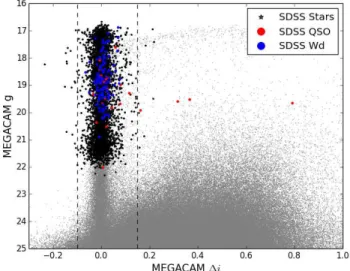
In order to quantify the range of concentration index needed to extract point sources, a set of spectroscopi-cally classified stars was queried from the SDSS. A plot of concentration index versus g-band magnitude is shown in Figure 1, where the black stars are stellar sources from the SDSS, red circles are QSOs from Pˆaris et al. (2014), and blue circles are spectroscopically confirmed
Figure 1. Concentration index, ∆i, vs. g-band magnitude for NGVS sources (gray) and stellar objects from SDSS (black). A narrow stellar sequence centered on ∆i = 0 is apparent, along with a broad cloud of background galaxies at fainter g-band magnitudes. Only 100,000 point sources from the NGVS are plotted for clar-ity. The dashed lines show our selection window for NGVS point sources, consistent with Durrell et al. (2014).
WDs from Kleinman et al. (2013). The dashed lines show the range in concentration index used by Durrell et al. (2014) to identify point sources:
−0.1 ≤ ∆i ≤ +0.15. (1)
Figure 1 shows that this selection is in excellent agree-ment with the location of the SDSS-selected point sources, including 99.3% of SDSS stars. Applying this selection on concentration index to the NGVS catalog returns 5.3 million point-like objects brighter than g = 24.5.
Note that Figure 1 also shows the saturation limit of the NGVS long exposures (g ∼ 17.5) as noted in Liu et al. (2015). The saturation causes photons to spill into adjacent pixels, which in turn leads to a more extended object, and hence a trail scattering toward positive ∆i values.
2.2. The GALEX Ultraviolet Virgo Cluster Survey
(GUViCS)
The UV point-source catalog used in this study is based on the GALEX Ultraviolet Virgo Cluster Survey (GU-ViCS; Boselli et al. 2011) catalog of Voyer et al. (2014), which includes data for 1.2 million point sources. The GUViCS survey itself, which consists of UV photome-try in both the near-UV (λeff = 2316 ˚A) and far-UV (λeff = 1539 ˚A) channels of GALEX, is an amalgama-tion of imaging from multiple programs, including the All Sky Imaging Survey (AIS), the Medium Imaging Sur-vey (MIS), the Deep Imaging SurSur-vey (DIS), the Nearby Galaxies Survey (NGS) and various GALEX PI programs (see Morrissey et al. 2007 for details on these surveys). Although the Virgo cluster region was fully covered by the AIS early in the mission lifetime, the GUViCS team was awarded time in 2010 to cover the NGVS footprint to a depth equivalent to that of the MIS. In all, GUViCS
spans an area of ∼ 120 deg2 centered on M87 and cov-ers most of the NGVS field, although some regions were avoided due to the presence of bright stars that would have saturated the GALEX detectors.
To maximize the point-source depth, only those detec-tions with the highest signal-to-noise ratio for a given object were retained. The final catalog contains the up-dated NUV photometry to a depth of mNUV ≃23.1 mag, and the previously acquired AIS FUV photometry to a depth of mFUV ≃19.9 mag. Only the deeper NUV pho-tometry was used to select candidates because just 41% of objects were detected in the FUV. For reference, the instrumental resolution in the NUV band is ∼ 4′′–6′′, with a median of 5.′′3 (e.g., Bianchi et al. 2014).
2.2.1. Bright Stellar Sources
In assembling the GUViCS point-source catalog, Voyer et al. (2014) removed 12 211 bright foreground stars that appeared in the SIMBAD database. This decision was appropriate given that their immediate science drivers were extragalactic in nature. Here, however, we are in-terested in matching the optical and UV photometry for a highly complete sample of stars, so the GUViCS cata-log was combined with the hot star catacata-log of Bianchi et al. (2011).
2.2.2. Multiple Matches
When matching the catalogs, there are two situations in which a multiple match can occur. The first, and most common, case is when multiple optical counterparts are attributed to a single GUViCS source. Indeed, the dif-ferences in spatial resolution and survey depth between the two catalogs mean that a number of NGVS objects are often matched to a single GUViCS object. This is not a rare occurrence given the depth of the NGVS data. The second, more infrequent, case is when multiple GU-ViCS sources are attributed to a single NGVS source. In either case, multiple matches are discarded because the optical-UV colors are compromised and must be excluded from our analysis. In all, matching the point-source cat-alogs from NGVS and GUViCS leads to 104 050 unique matches.
2.2.3. Spurious Matches
The high spatial density of the optical data means that there is a possibility that two unrelated sources may be matched (i.e, a spurious match). The likelihood of spuri-ous matches was estimated in two ways. First, a collec-tion of cutouts of one square degree from the GUViCS sample were selected, and one degree was added to both their right ascension and declination. The resulting tes-sellated cutout was then matched to the NGVS catalog and the spurious match rate was calculated as the total matches divided by the total number of points within the square degree offset. Repeating this exercise for five different pointings gives a spurious match rate of ∼2%
A second method to estimate the spurious match rate used a Monte Carlo approach. A 0.5 deg2 field contain-ing both GUViCS and NGVS data was used to assess the spatial density of both catalogs. The NGVS data were first replaced by an equal number of randomly gen-erated coordinates using the random.uniform function in Python. A nearest-neighbors algorithm was then ap-plied to the resulting coordinates in order to determine
the distance to the three nearest mock optical objects for each GUViCS object. If the distance to one of the three nearest neighbors was less than three arcseconds, then it was considered to be a match. This exercise was repeated 100 times for each GUViCS point. The average spurious match rate found in this way is ∼3%.
These methods suggest that the contamination from spurious matches is roughly 2–3%. Of course, the ac-tual contamination rate will be lower than this because the colors resulting from spurious matches are likely to be very odd and inconsistent between different indices. This was tested explicitly for the WDs selected from the NGVS-GUViCS catalog by matching 100 000 GU-ViCS objects to random NGVS objects; in this case, only 0.27% of matched objects would have been identified as candidate WDs. Scaling this to the number of objects in the NGVS-GUViCS matched sample shows that we expect less than one spurious match to be identified as a WD candidate.
2.3. Proper Motions: The Sloan Digital Sky Survey
Proper motions for objects in the NGVS were cal-culated by comparing their coordinates with those ob-tained from the SDSS DR7 (Abazajian et al. 2009). This provides the longest possible baseline, since subsequent SDSS data releases used more recent observations (Munn et al. 2014). The elapsed time between the SDSS and NGVS imaging ranges between 3 and 9 years, with an average of ∼ 7 years.
Deriving positions and epochs for the NGVS is not entirely straightforward because the final NGVS images were created by stacking individual frames with relatively short exposure times, whereas the SDSS images are com-posed of single draft scans. In some cases, the NGVS data acquisition process stretched over a period of a few years; in those instances, objects with high proper mo-tions can be smeared in the direction of motion. In order to mitigate errors in positions caused by this effect, we restricted our analysis to only those fields in which all images were acquired within a single observing season.
2.3.1. Comparison to the USNO Catalog
In order to check the accuracy of the NGVS-SDSS proper motions, our measurements were compared to those from the United States Naval Observatory (USNO) catalog (Munn et al. 2014), which partially overlaps with the NGVS. The USNO proper motions were computed from SDSS positions and follow-up observations obtained with the Steward Observatory Bok 90 inch telescope. Their images were acquired in the r-band with an aver-age baseline of six years; the quoted statistical uncertain-ties on the proper motions range between 5 mas yr−1for brighter objects (r ∼ 18) and 15 mas yr−1for the faintest objects (r ∼ 22). The USNO catalog, which is complete to r ∼ 22 (δ < 8.5), is the deepest proper motion survey currently available in the NGVS footprint.
A comparison between the proper motions derived in this work and those from the USNO catalog is shown in Figure 2.Also plotted are representative error bars for three g-band magnitude bins in order to show the mag-nitude dependence of the derived proper motion errors.
Figure 2. Comparison of proper motions derived from the NGVS and SDSS (abscissa) to those from the USNO-B catalog (Munn et al. 2014, ordinate). The residuals are plotted on the y-axis as the difference between proper motion measurements. Representative error bars for three g-band magnitude bins (17, 19, and 21) are also plotted.
At bright magnitudes the resulting average error is ∼6 mas yr−1 in both RA and DEC, and this increases to ∼12 mas yr−1 in the faintest bin.
2.3.2. Proper Motion Errors
To quantify the uncertainties associated with the method described above, a sample of spectroscopically confirmed QSOs from the SDSS was compiled from Pˆaris et al. (2014) over the magnitude range shown in 2. QSOs are point sources but are, of course, extragalactic in na-ture and so have negligible proper motions. The mean proper motions of the QSOs within the NGVS field in right ascension and declination are 3.3±0.4 and 1.2±0.3 mas yr−1, respectively. However, these errors are rather small compared to the range of proper motion examined in this paper and thus should not affect our findings. In our analysis, only those objects having combined SDSS positional errors of less than 0′′.1 were selected. With an average baseline of ∼ 7 years, this corresponds to a maximal uncertainty on proper motion of ∼ 15 mas yr−1.
3. SELECTION OF WHITE DWARF CANDIDATES
In this section, we describe the methodology used to identify WD candidates in the catalogs described in §2. Each selection method is designed to probe different re-gions of the WD luminosity function by applying sim-ple color, and hence temperature, selections. Candidates were selected in three ways: (1) by using the NGVS pho-tometry alone, which probes the hottest and youngest WDs (Tef f > 12,500 K); (2) by combining the NGVS with UV photometry from GUViCS, which selects ob-jects over a wider temperature range (Tef f > 9,500 K); and (3) by using proper motions derived from the NGVS and SDSS, which allows for a selection over all tempera-tures, but is limited to sources with first epoch positions needed for proper motion measurements. We conclude with a brief discussion of possible contamination by other point-like objects.
3.1. Method 1: Selection from the NGVS Color-Color
Diagram
The identification of WD candidates from the NGVS was performed using a color-color selection in the (u∗−g),
Figure 3. Color-color diagram of point sources in the NGVS (black dots). Also shown are WDs (blue), QSOs (red), and stars (magenta) selected from the SDSS inside the NGVS footprint. The dashed lines indicate our selection region for candidate WDs in the NGVS based on the sample of spectroscopically confirmed WDs from Kleinman et al. (2013).
(g − i) plane. Such a color-color diagram can be seen in Figure 3, which includes spectroscopically confirmed WDs (blue; Kleinman et al. 2013), QSOs (red; Pˆaris et al. 2014), and stars from SDSS DR7 (magenta; Abazajian et al. 2009).
Our color-color selection is shown by the black dashed lines in Figure 3. This dual color selection — (g−i) ≤ 0.4 and (u∗−g) ≤ 0.5 — minimizes contamination by QSOs and main-sequence stars while maximizing the number of WDs. The total number of WD candidates identified using this approach is 1209.
3.2. Method 2: Selection from NGVS-GUViCS
Color-Color Diagram
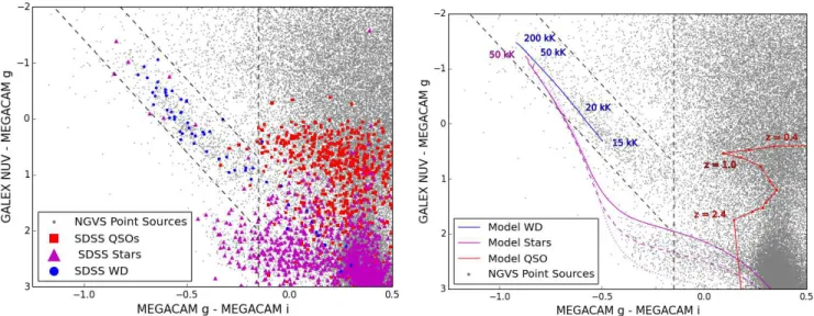
WD candidates in the NGVS-GUViCS catalog were selected by applying color cuts to the point-source cat-alog described in §2.2. The left hand panel of Figure 4 shows the location of spectroscopically confirmed WDs, QSOs, and stars from SDSS (see above). The right hand panel shows the corresponding model tracks that were specifically computed in the NGVS and GALEX colors from the grids of stellar and QSO models of Bianchi et al. (2009, 2011), which include high-gravity WD mod-els computed with the TLUSTY code (Hubeny & Lanz 1995), main-sequence and giant star model atmospheres computed with the Kurucz code (Kurucz 1993), and var-ious QSO templates. Comparing the left and right hand panels of Figure 4 shows that the models and observa-tions are generally in good agreement.
The black dashed lines in Figure 4 show the color cuts used to select WD candidates from the NGVS and GUViCS photometry. This selection methodology was adopted after visually inspecting the locations of the spectroscopically confirmed objects in the (g − i), (NUV−g) plane, with the goal of minimizing contamina-tion from QSOs and hot subdwarfs (see §3.4 for further discussion). A magnitude cut of g < 24.5 was also im-posed to minimize contamination from background
ob-jects. Furthermore, all objects with (g − i) < −0.15 were selected, which isolates the bluest objects in the NGVS data set. An additional selection, indicated by the diago-nal dashed lines, was then applied to separate the bluest main-sequence and subdwarf stars from the WDs. One final cut was imposed on the UV data by only selecting objects with uncertainties below 0.3 mag in the NUV channel. In all, these cuts result in the selection of 832 WD candidates.
A final addition to our sample of WD candidates was made using the results from Bianchi et al. (2011). A further 24 candidates were added by applying the same color cuts to the shallower GALEX AIS data, bringing the total number of candidates up to 856. Recall that this step is required because Voyer et al. (2014) removed bright stars in assembling the GUViCS point-source cat-alog. Matching these objects to SDSS DR12 reveals that 77 have spectroscopic measurements. Of these, 52 have been confirmed as WDs, nine as QSOs, and 10 as other types of hot stars, and six had S/N ratios less than four (see §3.4 for further discussion)
3.3. Method 3: Selection from NGVS-SDSS Proper
Motions
Our final selection method relies on the reduced proper motion diagram (RPMD) — a distance-independent metric that can be used to separate WDs from main-sequence stars and QSOs based on their photometry and proper motions. The reduced proper motion, H, relates the apparent magnitude, m, and the proper motion, µ, in arcsec yr−1, to the tangential velocity, v
t, in km s−1, and absolute magnitude, M :
H = m + 5 log µ + 5
= M + 5 log vt−3.379. (2) The RPMD is a useful tool for separating WDs from main-sequence stars due to their faint absolute luminosi-ties (Oppenheimer et al. 2001; Vennes & Kawka 2003; Kilic et al. 2006; Rowell & Hambly 2011; Limoges et al. 2015; Munn et al. 2017). The selection of WD candi-dates can be made by combining the observed magni-tudes, colors, and proper motions, and comparing them to model absolute magnitudes and tangential velocities. Model absolute magnitudes were calculated using the color-absolute magnitude relations from Holberg & Berg-eron (2006),Kowalski & Saumon (2006),Tremblay et al. (2011), and Bergeron et al. (2011)1 and combining an adopted tangential velocity to separate WD candidates. This can be seen in Figure 5, where the black lines rep-resent tangential velocities of 20 km s−1, 40 km s−1, and 200 km s−1 — values that are representative of the thin disk, thick disk, and halo, respectively (Harris et al. 2006). Also plotted in Figure 5 is a dashed line defined by Kilic et al. (2006); WDs are expected to fall below this relation. As expected, the large number of known main sequence stars and QSOs in our sample are found above the dashed line.
Using a tangential velocity cut of vt= 30 km s−1, we find a RPMD-selected sample of 342 WD candidates.
Figure 4. (g − i, NUV – g) color-color diagram for the matched NGVS-GUViCS point-source objects (gray). Left: Spectroscopically confirmed SDSS WDs (blue circles), QSOs (red squares), and stars (magenta triangles) are shown in relation to the NGVS-GUViCS objects. Right: Model tracks show the expected locations of WDs (blue) (Hubeny & Lanz 1995), QSOs (red) (Bianchi et al. 2009), and for stars of various surface gravities (magenta) (Kurucz 1993). The WD track, for log g = 8.0, is plotted for temperatures between 15,000 and 200,000 K. The nonlinearity of the temperature-color relation is apparent from the identified temperatures. The model QSO colors are plotted as a function of redshift, with values between 0 and 4. Model stars with solar metallicity and log g = 5, 4, and 3 are indicated by the solid, dashed, and dotted magenta lines, respectively. The black dashed lines indicate the color cuts applied to the NGVS-GUViCS data in order to select candidate WDs.
Figure 5. Reduced proper motion diagram for WD candidates. Spectroscopically confirmed WDs, QSOs, and stars are plotted as in Figure 4. Red triangles are halo candidates selected in this work as detailed in §5. Solid lines represent tracks for model WDs with a pure hydrogen atmosphere with vt = 20, 40, and 200 km s−1 from Holberg & Bergeron (2006).
3.3.1. Common Proper Motion Pair
The selection method also yielded one common proper motion pair, SDSS J122319.19+050121.4 and SDSS J122319.57+050121.3. These objects can be important for the study of type Ia supernovae progenitors, and also allow for the study of mass loss during the late stages of stellar evolution by constraining the IFMR (e.g., Finley & Koester 1997).
Visual WD binaries are rather rare, and represent roughly 5-6% of the total number of binary pairs (Sion et al. 1991). The SDSS has the largest sample of wide dou-ble degenerate binaries to date. Baxter et al. (2014)
se-lected 53 candidate double degenerate pairs within SDSS DR7.
The WDs in our observed pair have an estimated dis-tance of 153±5 pc, a separation of 5.′′8, and a tangential velocity of 67±2 km s−1— consistent with being a mem-ber of the thin disk. An SDSS spectrum is also available for J122319.57+050121.3 and confirms it to be a WD. Other calculated parameters are presented in Table 2, and show that the two WDs are consistent with being a double degenerate binary.
3.4. Sources of Contamination
As Figures 3– 5 show, some objects that are not WDs can still fall within our adopted selection regions. The primary source of contamination at very blue colors is O-subdwarf (sdO) stars. These stars are thought to be the cores of red giants that ejected their surrounding shell prior to reaching the AGB phase (Heber 2009). At redder colors, the most common contaminants are QSOs with emission lines that fall in the u∗ and g bands.
The contamination rate for each method was estimated by matching the WD candidates to a compendium of spectroscopic redshift measurements available for objects in the NGVS footprint. This NGVS spectroscopic cata-log includes redshifts in SDSS DR12, NED, and numer-ous NGVS programs that targeted the Virgo cluster (for more details, see Raichoor et al. 2014).
Table 3 summarizes the results of matching the WD candidates selected by each method to the NGVS spec-troscopic catalog. From left to right, the columns of this table record the selection technique, the tempera-ture range probed by each method (see §4.3), the num-ber of WD candidates, the numnum-ber of WDs matched to the NGVS spectroscopic catalog, the number of spectro-scopically confirmed QSOs and main-sequence stars, and
Table 2
Common Proper Motion Pair Properties
SDSS ID u (AB mag) g (AB mag) i (AB mag) z (AB mag) Teff(K) d (pc) vt(km s−1) µRA(mas/yr) µDEC(mas/yr) J122319.19+050121.4 18.46±0.02 18.00±0.01 18.25±0.01 18.53±0.04 10500±1000 153+5−3 67.1±2.3 -91.4±0.4 12.9±0.4 J122319.57+050121.3 19.20±0.028 18.82±0.01 18.82±0.01 18.98±0.05 8500±500 152+5
−3 66.6±2.3 -91.4±0.6 13.1±0.5
Note. — Magnitudes are from the SDSS.
180 182 184 186 188 190 192 1944 6 8 10 12 14 16 18 20 DEC (deg) NGVS 180 182 184 186 188 190 192 194 RA (deg) 4 6 8 10 12 14 16 18 20 NGVS-GUViCS 180 182 184 186 188 190 192 194 4 6 8 10 12 14 16 18 20 NGVS-SDSS
Figure 6. WD candidates from the NGVS (left), NGVS-GUViCS (middle), and NGVS-SDSS (right) selection methods are plotted on the sky. The black lines show the approximate boundaries of the NGVS.
Table 3
Contamination Rates for WD Selection Methods
Method Teff NWD vr QSOs Stars fc
(K) matches (%)
NGVS &12 250 1209 86 3 9 14 NGVS-GUViCS &9500 856 77 9 4 17 NGVS-SDSS All 342 76 1 2 4
Note. — Teff range determined from (g − i) color selection.
the overall contamination rate, in percent, for the sub-set of WD candidates having measured radial velocities. After inspecting the spectra of these objects, we con-clude that one likely WD was misclassified as a brown dwarf, and three more likely WDs were classified as B-type stars from spectra with low signal-to-noise (i.e., S/N ∼3). The resulting contamination rate is 14-17% for the photometrically selected samples and drops to 4% when proper motions are included. However, as these values are dependent on the completeness of the SDSS spec-troscopic catalogs they should be treated as lower limits and are meant to show the relative contamination rates between the selection methods.
4. PHOTOMETRIC PROPERTIES
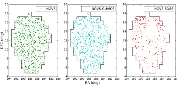
This section discusses photometric properties derived for the three WD catalogs described in §3. The distri-bution of the WDs on the sky is presented in Figure 6. While the NGVS distribution (left) is rather uniform, the voids in the NGVS-GUViCS sample (center)
repre-sent the location of bright stars that were avoided dur-ing data acquisition (see §2.2). Furthermore, the NGVS-SDSS catalog (right) shows the location of the fields for which the stacked images were composed of exposures taken over more than one observing run (see §2.3).
4.1. Distributions of Apparent Magnitude
The distribution of g-band magnitudes for the WD samples obtained using our three different methods is shown in Figure 7 (green, red, and cyan histograms). For comparison, the black histogram shows the distri-bution found when using the subsample of WDs from Bianchi et al. (2011) in the NGVS footprint; recall that this sample is based on a GALEX/AIS-SDSS color-color selection. Finally, we show (as the blue histogram) the sample of spectroscopically confirmed WDs from SDSS in the NGVS footprint from Kleinman et al. (2013).
The NGVS-selected LFs shown in Figure 7 reach to g ∼ 22-24.5, with the precise limit depending on the selection method. We emphasize that this is much brighter than the NGVS detection limits. Source completeness in the NGVS has been discussed in (Ferrarese et al. 2012 and Ferrarese et al. 2017, in press), but Figure 7 of the former paper demonstrates that the 10σ detection limit for point sources in the NGVS is g ≃ 26, or 1.5–4 mag fainter than the samples considered here (which were truncated at g = 24-25 mag in order to minimize contamination by background galaxies; see Figure 1). Thus, our WD samples are essentially 100% complete to our adopted limits.
17 18 19 20 21 22 23 24 25
MEGACAM g mag (AB)
0 50 100 150 200 250 300 N Bianchi et al. 2011 NGVS NGVS-SDSS NGVS-GUViCS Kleinman et al. 2013
Figure 7. Magnitude distributions for WD candidates selected using our three methods described in §3 (green, cyan and red his-tograms). For comparison, we show the distributions obtained for the NGVS footprint using the SDSS spectroscopic catalog of Klein-man et al. (2013), and GALEX AIS photometric selection from Bianchi et al. (2011). The latter have been scaled to correct for incompleteness.
Figure 7 highlights the depth of the combined NGVS and GUViCS data. All five histograms agree quite well brighter g ∼ 19; however, fainter than this, the SDSS spectroscopy and GALEX/AIS-SDSS samples clearly suffer from incompleteness. The three NGVS samples described in the previous section all peak well below this magnitude, and the sample of WDs selected entirely from the NGVS continues to rise down to the magnitude limit imposed in §2. By contrast, the NGVS-GUViCS sample shows a gradual fall-off beginning at g ∼ 22 — a result of the GUViCS survey limit. Similarly, the decline in the number of NGVS-SDSS candidates is an artifact of the SDSS completeness limit.
A noteworthy feature of Figure 7 is the large number of objects in faintest bin of the NGVS-selected sample. As Figure 1 shows, the measured concentration indices for objects fainter than g ∼ 24 are much noisier than those for brighter objects. This suggests that background sources may dominate the NGVS-selected sample in the faintest bin. For the remainder of this paper, we will discuss our findings with, and without, this faint bin.
4.2. Photometric Distances
Distances to a subset of the candidates were esti-mated using theoretical color-absolute magnitude rela-tions from Holberg & Bergeron (2006). Absolute mag-nitudes were estimated using a 0.6M⊙ pure hydrogen atmosphere model (Holberg & Bergeron 2006) and were combined with the apparent magnitude to derive a dis-tance,
d = 100.2(m−M +5−Ag). (3)
Here m refers to the g-band magnitude, M is the the-oretical absolute magnitude from the model of Holberg & Bergeron (2006), and Ag = 0.066 mag is the average g-band extinction coefficient in the NGVS field.
1000 0 1000 2000 3000 4000 5000 6000 7000 Distance (pc) 0 20 40 60 80 100 N NGVS NGVS g < 24 NGVS-SDSS NGVS-GUViCS
Figure 8. Photometric distances for the WD candidates selected as described in §3. Absolute magnitudes have been calculated us-ing the Holberg & Bergeron (2006) color-absolute magnitude rela-tionship. The NGVS sample (green) is plotted with (dotted) and without (solid) the g=24.5 mag bin.
The distributions in Figure 8 can be explained by a combination of the survey parameters and selection methods. For instance, the NGVS-selected sample probes hotter candidates to fainter g-band magnitudes, and hence larger distances, than the NGVS-GUViCS sample. The NGVS-SDSS proper motion method is sen-sitive to objects with large proper motions, which results in the preferential selection of nearby objects.
It is important to note that the model color-absolute magnitude relation becomes very steep at high tempera-tures. For blue objects, this leads to large uncertainties in the derived absolute magnitudes and distances: i.e., a change in (g − i) color of just 0.01 mag can result in a 1 mag change in absolute magnitude. These errors can lead to a flattening of the distance distribution, yielding some objects with significantly overestimated distances.
Another feature of Figure 8 is the large number of ob-jects in the dotted green histogram that lie at 4 kpc. This histogram represents the faintest magnitude bin (24.0 < g < 24.5) from Figure 7 and, as previously discussed, many of these objects are thought to be contaminants. We therefore believe that this feature is probably not real.
4.3. Effective Temperatures
Effective temperatures for the WD candidates were derived by fitting model spectral energy distributions (SEDs) to the u∗giz photometry as in Hu et al. (2013). We used the cooling models of Holberg & Bergeron (2006) which span the temperature range 100 000 to 1500 K. This broad range is sampled in increments of: (1) 5000 K between 100 000 and 20 000 K; (2) 500 K be-tween 17 000 and 5500 K; and (3) 250 K bebe-tween 5500 and 1500 K. Best-fit effective temperatures were com-puted via χ2minimization after applying a vertical shift equal to the mean difference between the model and ap-parent magnitudes. The left panel of figure 9 shows an example of this derivation for six candidates over a wide temperature range. A comparison between the temper-atures derived via this method and those derived from
14.5 15.5 16.5 17.5 4750.0 K 13.6 14.0 14.4 14.8 6500.0 K 13.2 13.4 13.6 13.8 7500.0 K 11.9 12.1 12.3 12.5 10500.0 K 3000 5000 7000 9000 10.4 10.8 11.2 11.6 20000.0 K 3000 5000 7000 9000 9.8 10.2 10.6 11.0 25000.0 K Wavelength ( ) M (AB Mag) 5000 10000 15000 20000 25000 30000 35000
Teff (Kleinman et al. 2013) 5000 10000 15000 20000 25000 30000 35000
Teff (This Work)
Figure 9. Right: Example SED fits used to derive temperatures for WD candidates. The red lines are the best-fitting 0.6 M⊙SEDs for a pure hydrogen from Holberg & Bergeron (2006) and the black points are the observed magnitudes after applying a vertical shift. Left: Comparison between the resulting temperatures (y-axis) and those derived from spectroscopy by Kleinman et al. (2013).
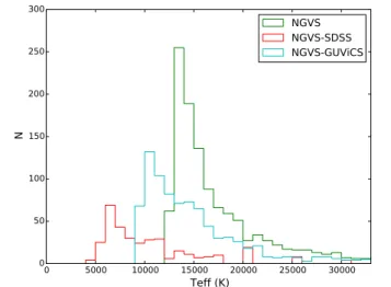
0 5000 10000 15000 20000 25000 30000 Teff (K) 0 50 100 150 200 250 300 N NGVS NGVS-SDSS NGVS-GUViCS
Figure 10. Temperature distributions for WD candidates based on SED fitting.
SDSS spectroscopy by Kleinman et al. (2013) is pre-sented in the right panel of 9. Overall, our method favors cooler temperatures than those measured spectroscopi-cally. However, this effect is likely a result of the fact that both methods use different model atmospheres.
The distributions of best-fit temperatures for our three WD samples are shown in Figure 10. The NGVS-selected sample consists of 1209 WD candidates with (g − i) < −0.4, corresponding to temperatures Teff &12 500 K. By contrast, the (g − i) < −0.15 selection adopted for the NGVS-GUViCS sample (856 objects) corresponds to temperatures Teff &9500 K. The sample of 342 WD can-didates selected from NGVS-SDSS proper motions selec-tion imposed no color cut, so there is no restricselec-tion on temperature in this case.
5. CHARACTERIZING THE WHITE DWARF CANDIDATES
In this section, we describe our efforts to identify disk and halo WD candidates using their scale heights, proper motions, and space velocities.
1000 0 1000 2000 3000 4000 5000 6000 7000 Scale Height (pc) 0 50 100 150 200 N NGVS NGVS g < 24 NGVS-SDSS NGVS-GUViCS
Figure 11. Calculated scale heights based on distance estimates from the Holberg & Bergeron (2006) model.
5.1. Photometric Samples
The numbers of halo WDs in the NGVS and the NGVS-GUViCS samples were estimated using distances derived from the models of Holberg & Bergeron (2006). Bovy et al. (2012) have recently used G dwarfs as tracers of the stellar disk and found that the population is well fitted by an exponential up to a scale height of ∼ 1 kpc. The calculated scale heights for each sample can be seen in Figure 11, where the black dotted line represents the chosen boundary between the disk and halo popu-lations. The depth of the NGVS sample results in the largest fraction of halo WDs, with 64% of objects having an estimated scale height in excess of 1 kpc. This is fol-lowed by a halo fraction of 28% in the NGVS-GUViCS sample, and just 0.3% in the NGVS-SDSS proper mo-tion sample. This result reflects the selecmo-tion methods discussed in §3. The NGVS and NGVS-GUViCS sam-ples are much deeper than the NGVS-SDSS sample and hence probe larger distances.
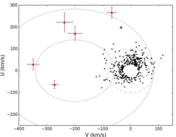
Figure 12. Galactic space velocities calculated under the assump-tion of zero radial velocity for NGVS-SDSS WD candidates (black). Halo candidates selected using the reduced proper motion diagram are shown as red triangles. The cyan dot-dashed and blue dashed ellipses represent the 2-σ velocity ellipsoids for the thick and thin disk populations while the dotted black lines show the 1- and 2-σ velocity ellipsoids for the halo, all from Chiba & Beers (2000).
5.2. Kinematic Sample
5.2.1. Reduced Proper Motion Diagram
The RPMD can be used to characterize WDs as prob-able disk or the halo members based on their estimated tangential velocities (e.g., Kilic et al. 2006; Rowell & Hambly 2011). Figure 5 shows the model curves of Hol-berg & Bergeron (2006) for 0.6M⊙ WDs with a pure hydrogen atmosphere and tangential velocities of 20, 40, and 200 km s−1 — appropriate for the thin disk, thick disk, and halo, respectively.
A total of seven halo WD candidates lie below the vt= 200 km s−1relation. A visual inspection of the SDSS and NGVS imaging reveals one of the objects to be a binary that is resolved in the NGVS but unresolved in the SDSS, leading to a spurious proper motion. The properties of the remaining six halo candidates are discussed in §6 and summarized in Table 4.
5.2.2. Galactic Space Velocities
It is possible to separate disk and halo stars using their Galactic space velocities (U, V, W) (e.g., Pauli et al. 2006). Since these velocity components are defined with respect to the Galactic center, it is necessary to transform their positions from equatorial (α, δ) to Galactic (l, b) coordinates (e.g., Johnson & Soderblom 1987). Needless to say, the transformation into the (U, V, W) frames requires both a proper motion and a radial velocity. Since radial velocities are not available for the vast majority of our WD candidates, we set ρ to zero. However, the contribution to U and V space velocity components is small at the fairly high Galactic latitude of the NGVS (b ∼ 75◦).
With this caveat in mind, the U and V velocities for our WD candidates are shown in Figure 12. The cyan dot-dashed and blue dashed ellipses represent the 2-σ velocity ellipsoids for the thick and thin disk populations, respectively. The dotted black lines show the 1- and 2-σ
Figure 13. SDSS-NGVS luminosity function (red) compared to those derived by Harris et al. (2006) (cyan) using SDSS DR3 and Rowell & Hambly (2011) (green) using the SuperCOSMOS survey.
velocity ellipsoids for the halo. These velocity ellipsoids were taken from Chiba & Beers (2000).
The six halo WD candidates identified from the RPMD are shown as the red triangles in Figure 12. Of these six objects, five fall inside the 2-σ velocity ellipsoid of the Galactic halo, while the sixth lies just outside.
5.3. Sample Completeness and Luminosity Functions
Sample completeness can be assessed using the V/Vmax method (Schmidt 1968) which gives the ratio of the volume out to a given detected WD to the volume out to the distance the WD would have at the detection limit of the survey. Vmax can be calculated using the methodology described by Rowell & Hambly (2011) and Hu et al. (2013): Vmax = βR rmax rmin ρ ρ⊙R 2dR, (4) Here β is the survey area as a fraction of the total sky,
ρ
ρ⊙ is the stellar density along the line of sight, R is
the distance, and rmin and rmax are the minimum and maximum distances for which an object would fall within the survey limits. These distances are defined as
rmin = 100.2(mmin−M +5−Ag) (5) and
rmin = 100.2(mmax−M +5−Ag) (6) where mmax and mmin are the faint and bright limits of the survey. The stellar density for the disk is assumed to be ρ ρ⊙ = exp h −|R sin b+Z⊙| H i , (7)
where H is the scale height of the disk, R is the dis-tance to the object from the model of Holberg & Berg-eron (2006), b is the Galactic latitude, and Z⊙ = 20 pc is distance of the Sun above the Galactic plane (Reed 2006).
Using this method, we find DVmaxV E ±1/(12N )1/2 = 0.39 ± 0.02 for the sample of N = 342 kinematically se-lected WD candidates. For a uniform distribution, the
Figure 14. Luminosity function for halo candidates selected using the NGVS-SDSS proper motions.
mean value should be 0.5, suggesting some incomplete-ness in the sample. This incompleteincomplete-ness is likely a con-sequence of our selection method, which removes many faint objects due to the large uncertainty in their SDSS positions.
The maximum volume, Vmax, can be used to con-struct a luminosity function that, once integrated, yields a space density. The number density of objects, φ, can be expressed as the sum of the inverse maximum volumes:
φ = PN i
1
Vmax,i. (8)
The uncertainty in the number density, σφ, can then be calculated using Poisson statistics (Rowell & Hambly 2011): σ2 φ = PN i 1 V2 max,i. (9)
The resulting luminosity function must then be rescaled to account for the absence of WDs with tangen-tial velocities less than 30 km s−1 in our sample selected by proper motion. This scale factor was calculated us-ing the Besan¸con WD catalog (explained in more detail below), which suggests that the fraction of WDs hav-ing tangential velocities above 30 km s−1 in the NGVS field is 0.746. This value is in good agreement with the value of 0.726 obtained by Harris et al. (2006) for the SDSS DR3 field. The luminosity functions for our disk and halo WD candidates are shown in Figures 13 and 14, respectively, and are discussed below.
6. DISCUSSION
6.1. Comparison to the SDSS and SuperCOSMOS
Luminosity Functions
Figure 13 compares the luminosity function for the sample of WD candidates selected from SDSS-NGVS proper motions to those obtained with SDSS DR3 (Har-ris et al. 2006) and the SuperCOSMOS survey (Rowell & Hambly 2011). This comparison shows a discrepancy at the bright end of the luminosity function, although the faint ends are consistent. The discrepancy at the bright end is a likely a consequence of the high Galactic latitude of the NGVS field combined with the geometry of the Milky Way disk. That is to say, the SDSS and SuperCOSMOS surveys reached to lower Galactic lati-tudes, which contain different fractions of thin and thick
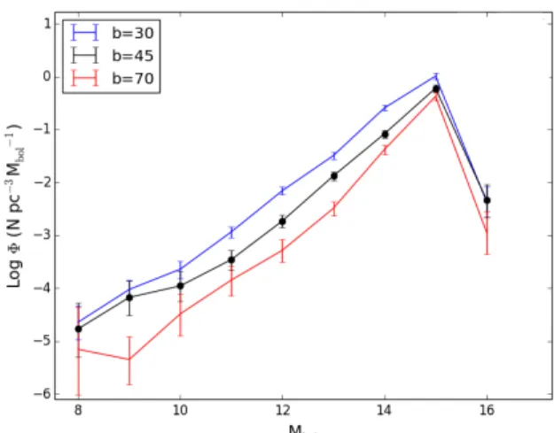
Figure 15. WD luminosity functions calculated with the Be-san¸con model for three different Galactic latitudes.
disk stars.
We explored the importance of this effect using the Be-san¸con model. Figure 15 shows the luminosity function of WDs at b = 30◦, 45◦, and 70◦ while keeping all other parameters of the model fixed. The luminosity functions at each Galactic latitude can be seen as the blue, black, and red curves in Figure 15. This exercise demonstrates that, at higher Galactic latitudes, there is a discrepancy at the bright end that is comparable to that seen in the observations, while the faint ends of the luminosity func-tions are nearly identical.
6.1.1. Number Densities
A number density for the thin disk was estimated by integrating the NGVS-SDSS luminosity function with H = 250 pc. Because this has been a customary choice in many previous studies, it allows for a direct comparison to earlier measurements. The resulting number density for the disk is then
φd= (2.81 ± 0.52) × 10−3 pc−3. (10) This value is consistent with several previous estimates: e.g., 2.36±0.27 × 10⁻³by Hu et al. (2013) and 3.19±0.09 × 10⁻³ by Rowell & Hambly (2011). It is somewhat lower than the estimates of 5.5±0.1 ×10⁻³, 4.6 ×10⁻³ and 3.4 ×10⁻³ from Munn et al. (2017), Harris et al. (2006) and Leggett et al. (1998), respectively, although this discrepancy is likely caused by the differing sightlines of the surveys, as explained above.
Assuming that the six high-velocity WDs belong to the halo (§5.2.2), the number density of halo WDs is estimated to be
φh= (7.85 ± 4.55) × 10−6 pc−3. (11) This value is marginally lower than the number densities of ∼ 4 × 10⁻⁵ pc−3 found by Harris et al. (2006) and 3.5±0.7× 10⁻⁵ pc−3 found by Munn et al. (2017). This is likely a result of our selection method, which rejected many faint objects with large proper motion errors. Our result is marginally higher than the number density of 4.4±1.3 × 10⁻⁶ reported by Rowell & Hambly (2011).
Of course, such comparisons should be treated with caution because they are highly dependent on survey pa-rameters. The number density relies mainly on the faint
Table 4
Properties of NGVS Halo White Dwarf Candidates
NGVS ID u∗(AB mag) g (AB mag) i (AB mag) z (AB mag) T
eff(K) d (pc) vt(km s−1) µRA(mas/yr) µDEC(mas/yr) J124516.62+170505.1 21.558±0.004 20.606±0.002 20.645±0.004 20.823±0.009 6500±500 406+4 −3 218±14 -18.7±5.0 -99.1±5.3 J121933.27+163829.4 21.724±0.004 21.277±0.003 21.375±0.006 21.501±0.017 7500±500 613+10 −9 293±35 -94.7±3.0 -62.4±2.9 J121955.46+151523.1 21.463±0.003 20.975±0.002 21.343±0.006 21.582±0.016 11000±1000 569+267−265 201±96 -59.2±2.7 -30.4±2.2 J122515.80+064849.2 20.924±0.003 20.661±0.002 21.075±0.005 21.324±0.014 10000±1000 758+7 −6 279±26 -71.3±3.4 -31.0±3.1 J123614.18+061135.0 20.547±0.002 20.204±0.002 20.711±0.004 20.941±0.014 9500±500 714+8 −7 267±21 -75.2±4.8 -53.9±4.6 J121455.93+125058.4 20.028±0.002 19.873±0.001 20.515±0.004 20.830±0.008 20000±3000 853+12 −11 423±98 44.3±3.4 -94.7±3.4
Note. — WD properties calculated for an assumed mass of 0.6M⊙.
end of the luminosity function, which is in turn depen-dent on survey depth. As the depth increases, the rel-ative contributions from the thin disk, thick disk, and halo will also change.
6.2. Model Comparisons
In this section we compare the number densities gener-ated by the TRILEGAL and Besan¸con stellar population synthesis models with the three samples of WDs selected in Section 3.
A TRILEGAL WD catalog was computed by generat-ing ten mock regions of 10 deg2(the maximum allowable survey area) covering the NGVS footprint. All other in-put parameters were left at their default values, including a Chabrier initial mass function, a Milky Way extinction model, and a three-component Galactic model, includ-ing squared hyperbolic secant thin and thick disks and an oblate halo. Due to the high Galactic latitude of the NGVS field, this sightline will include no bulge stars. Stars belonging to the mock catalog were deemed to be WDs if their log g > 7. Mock WDs were then assigned to the appropriate Galactic component — numbered 1 for the thin disk, 2 for the thick disk, and 3 for the halo. A Besan¸con WD catalog was constructed by generat-ing a region of 100 deg2, again centered on the NGVS footprint, with default parameters described in Robin et al. (2003). As with the TRILEGAL selection, WDs were identified by their high surface gravities. Objects were then divided into their respective Galactic component based on their designated population, with numbers 2-7 representing the thin disk, 8 representing the thick disk, and 9 representing the halo.
Three catalogs were generated by each model, and WDs were selected using the same color and magnitude selections described in Section 3. The resulting g-band magnitude distributions, described as number densities to account for variations in field area, are shown in Fig-ure 16.
The left hand panels show the comparison between the Besan¸con models and the NGVS (top), NGVS-GUViCS (middle), and NGVS-SDSS (bottom) WD candidates. Using the NGVS and NGVS-GUViCS catalogs as rep-resentations for the hot, young, WD population reveals a relatively good agreement between the model and ob-servations. The slightly larger number of observed WDs in the NGVS (top) and NGVS-GUViCS (middle) cata-logs is likely due to the fact that, as discussed in §3.4 and Table 3, both samples include a non insignificant fraction of contaminants (∼15%). Unfortunately, due to the lack of complete spectroscopic data to the limit of the NGVS survey, the contamination rate cannot be
ac-curately modeled. Additionally, as discussed in §4.1 and Figure 7, the NGVS-GUViCS sample is known to be in-complete below g∼22, which can explain the decline in observed WDs compared to the models.
Comparing the Besan¸con model to the NGVS-SDSS proper motion sample reveals a strong agreement at bright magnitudes with a divergence beginning around g∼19.5. This is a result of the cuts in proper motion error implemented to reduce contamination from other stellar sources. This effect has been accounted for in the black dashed line, which was calculated using the fraction of objects in each bin that passed our selection criteria and applied to the mock catalog. This shows that the model and observed counts are in agreement.
The right hand panels of Figure 16 compare the ob-served number densities to those computed using the TRILEGAL mock catalogs. The comparison between the observed densities of hot WDs from the NGVS and NGVS-GUViCS samples shows an overprediction by the TRILEGAL model, consistent with the results from Bianchi et al. (2011), who showed that this is a result of the IFMR adopted by TRILEGAL. This discrepancy is also apparent in the NGVS-SDSS proper motion sample, where the selection is not based on temperature.
Figure 16 also highlights the disagreement between the predicted numbers of halo WDs present in our catalogs. For example, TRILEGAL predicts 280 halo WDs in our catalog selected by proper motion selected, whereas the Besan¸con does not predict any. Although it predicts no halo WDs in our samples, the Besan¸con model does in-deed include them, but they are expected to be too faint and too cool to be detected in our survey. The discrep-ancy between observations and model likely arises from the method by which the mock halo WDs are generated from their main-sequence progenitors: i.e., through the IFMR, which is poorly constrained by observations. The IFMR used in the Besan¸con model predicts final halo WD masses of 0.7 M⊙, which would result in fainter model magnitudes. Observations have revealed a wide range of masses for halo WDs, and favor lower masses and hence higher luminosities (see, e.g Bianchi et al. 2011). For their sample of field halo WDs, Pauli et al. (2006) obtained masses of 0.35 − 0.51 M⊙, while Kilic et al. (2012) calculate masses of 0.62 M⊙ and 0.77 M⊙. Re-cent studies of the globular cluster M4 have established that WDs with masses of ∼ 0.5 − 0.55 M⊙ are currently being formed in halo environments (see, e.g Moehler et al. 2004; Bedin et al. 2009; Kalirai et al. 2009) and hence a model mass of 0.7 M⊙ does not accurately represent a halo environment.
17 18 19 20 21 22 23 24
g (mag)
0
1
2
3
4
5
6
#/sq. deg/0.5 mag
Besancon
All WDs Thin disk Thick disk NGVS WDs17 18 19 20 21 22 23 24
g (mag)
0
1
2
3
4
5
6
#/sq. deg/0.5 mag
TRILEGAL
All WDs Thin disk Thick disk Halo NGVS WDs17 18 19 20 21 22 23 24
g (mag)
0
1
2
3
4
5
6
#/sq. deg/0.5 mag
Besancon
All WDs Thin disk Thick disk NGVS-GUViCS WDs17 18 19 20 21 22 23 24
g (mag)
0
1
2
3
4
5
6
#/sq. deg/0.5 mag
TRILEGAL
All WDs Thin disk Thick disk Halo NGVS-GUViCS WDs18
19
20
21
g (mag)
0
1
2
3
4
5
6
#/sq. deg/0.5 mag
Besancon
All WDs Thin disk Thick disk NGVS-SDSS WDs18
19
20
21
g (mag)
0
1
2
3
4
5
6
#/sq. deg/0.5 mag
TRILEGAL
All WDs Thin disk Thick disk Halo NGVS-SDSS WDsFigure 16. Magnitude distributions for the NGVS (top), NGVS-GUViCS (middle), and NGVS-SDSS (bottom) WD catalogs compared to the TRILEGAL (right) and Besan¸con (left) mock catalogs. The observed WD candidates are shown in red, and the mock WDs are separated into the thin disk (cyan), thick disk (blue) and halo (green) respectively. In the lower panels, the dashed black curves show the mock WD samples after applying corrections to account for the incompleteness suffered by the data.
6.3. Thick Disk or Halo Membership?
The debate over whether halo WDs can be identified solely on the basis of their kinematics took on a renewed importance with the study performed by Oppenheimer et al. (2001), who used Galactic space velocities from WDs in the SuperCOSMOS Survey to conclude that as much as 2% of the “unseen” matter in the Galactic halo could arise from cool WDs. Bergeron (2003) and Bergeron et al. (2005) emphasized the importance of total stellar ages (i.e., main-sequence plus WD cooling ages) when char-acterizing WDs as belonging to the stellar halo, because many WDs with halo kinematics were so hot, and thus so young,as to call into question their association with the halo. On the other hand, if these WDs had lower than ex-pected masses then they could have ages consistent with a halo population, because they would have formed from less massive progenitors — objects with longer main-sequence lifetimes, and hence, longer main-main-sequence and WD cooling lifetimes. For example, a 0.6M⊙ WD would have an initial main-sequence mass of ∼ 2 M⊙and a life-time of ∼ 1 Gyr. By contrast, a 0.53M⊙ WD would have a main-sequence mass of 1 M⊙ and a lifetime approach-ing 10 Gyr (Dame et al. 2016). This simple example highlights the importance of accurate mass and distance measurements when assigning WDs to different compo-nents of the Galaxy.
Reyl´e et al. (2001) used the Besan¸con model to show that the sample of Oppenheimer et al. (2001) is likely dominated by the thick disk as opposed to the halo. Us-ing our Besan¸con mock catalog we compute the reduced proper motion for the mock WDs to determine the ex-pected number of thick disk objects that would be se-lected as halo candidates in our work. This exercise re-veals an expectation value of 1 WD, showing that the thick disk alone probably does not account for our ob-served sample of high velocity WDs.
The properties of the six halo WD candidates selected from our proper motions are summarized in Table 4. Temperature estimates were obtained by SED fitting as described in §4. Based on the derived temperatures, and assuming a 0.6M⊙ model with a pure hydrogen atmo-sphere, the inferred cooling ages range from 60 Myr to 6 Gyr. However, as previously noted, these values are highly sensitive to the adopted mass.
6.4. Comparison to Open and Globular Clusters
In environments where the WD luminosity function can be observed to faint magnitudes, WD ages can used to intercompare the star formation histories of different stellar systems or Galactic components (e.g., Hansen et al. 2013,?). Because star clusters are typically formed during a single burst of star formation, the location of the peak of the WD luminosity function provides an in-dicator of cluster age: i.e., the WD luminosity function in older stellar populations will peak at fainter magni-tudes for the simple reason that the WDs have had more time to cool (Bedin et al. 2009).
The stellar populations of globular and open clusters are often used as analogs for those of the halo and old disk, respectively, so it is of interest to compare their WD luminosity functions to those from our study. The WD luminosity functions for a representative globular cluster, M4, and an old open cluster, NGC 6791, are
shown in Figure 17. From the main-sequence turnoff of the clusters, M4 has been found to have an age of 12.0 ± 1.4 Gyr (Hansen et al. 2004), and NGC 6791 an age of ∼8 Gyr (Bedin et al. 2008). These ages are comparable to estimates for the age of the inner halo (12.5+1.4−3.4Gyr; ?) and that of the thin disk (7.4-8.2 Gyr; ?). The NGVS WD disk luminosity function from Figure 13 is shown in red. Note that the SDSS magnitudes for the disk candidates were converted to the Hubble Space Telescope filter system using transformations from Sirianni et al. (2005) and Lupton (2005)1, and a representative error bar is plotted at the peak of the luminosity function. The luminosity functions are normalized such that the peaks equal 1.
Bedin et al. (2008) note the double peak in the lumi-nosity function of NGC 6791, which they attribute to unresolved double degenerate binaries. These authors derive a cluster age of ∼6 Gyr — somewhat younger than the age of 8-9 Gyr found from the main-sequence turnoff. Garc´ıa-Berro et al. (2010) argue that this dis-crepancy can be resolved by considering22Ne separation in the cores of the cool WDs, which slows cooling and increases the derived age. Overall, Figure 17 shows that the NGVS disk luminosity function bears a close resem-blance to that of NGC 6791, including the faint peak. The luminosity function for M4 continues to rise beyond the disk turnoff, showing that many of the halo WDs remain undetected, presumably because the faintest ob-jects in the NGVS lack proper motion measurements due to the lack of deep first epoch positions.
7. CONCLUSIONS
We have used the deep imaging from the NGVS to identify and study WDs within the ∼100 deg2 NGVS footprint. WD candidates were identified using three dif-ferent techniques: (1) a sample of 1209 candidates were selected from the (g − i, u − g) color-color diagram for point sources based entirely on the NGVS photometry; (2) a sample of 856 candidates were selected from the (NUV−g, g − i) color-color diagram based on the NGVS and GUViCS surveys; and (3) a sample of 342 candidates were selected from the reduced proper motion diagram derived from NGVS and SDSS. Effective temperatures were calculated by SED fitting of the u∗giz NGVS mag-nitudes while photometric distances for all candidates were estimated using theoretical color-magnitude rela-tions from Holberg & Bergeron (2006).
Scale heights computed from these photometric dis-tances were used to separate the WD candidates into possible disk and halo subsamples. Doing so requires accurate photometry since, at the highest WD temper-atures probed by the NGVS, small errors in apparent magnitude translate into large errors in distance (i.e., the color-absolute magnitude relation becomes very steep in this temperature regime).
For the sample of WD candidates selected from the NGVS-SDSS proper motions, a selection based on tan-gential velocity was used to separate the disk and halo subsamples. Selecting candidates with a tangential ve-locity larger than 200 km s−1, we find six possible halo WDs. These candidates have relatively high
tempera-1 https://www.sdss3.org/dr10/algorithms/ sdssUBVRITransform.php