HAL Id: tel-01557535
https://tel.archives-ouvertes.fr/tel-01557535
Submitted on 6 Jul 2017HAL is a multi-disciplinary open access
archive for the deposit and dissemination of sci-entific research documents, whether they are pub-lished or not. The documents may come from teaching and research institutions in France or abroad, or from public or private research centers.
L’archive ouverte pluridisciplinaire HAL, est destinée au dépôt et à la diffusion de documents scientifiques de niveau recherche, publiés ou non, émanant des établissements d’enseignement et de recherche français ou étrangers, des laboratoires publics ou privés.
Molecular Density Functional Theory under
homogeneous reference fluid approximation
Lu Ding
To cite this version:
Lu Ding. Molecular Density Functional Theory under homogeneous reference fluid approximation. Theoretical and/or physical chemistry. Université Paris Saclay (COmUE), 2017. English. �NNT : 2017SACLV004�. �tel-01557535�
Molecular Density Functional Theory
under homogeneous reference fluid approximation
lu ding
Under the direction of
daniel borgis, luc belloni & maximilien levesque
an advanced molecular-scale liquid theory for solvation property prediction
Lu Ding: Molecular density functional theory under homogeneous reference fluid
When you are studying any matter, or considering any philosophy, ask yourself only, what are the facts and what is the truth that the facts bear out. Never let yourself be diverted either by what you wish to believe, or by what you think
would have beneficent social effects if it were believed. But look only, and solely, at what are the facts. — Bertrand Russell
Acknowledgements
First of all, I would like to express my most respectful gratitude to my thesis advisors, Daniel Borgis and Luc Belloni, who have developed the main theories used in this thesis and whose great knowledge of liquid theory as well as the genius way of thinking and explaining have given me a solid guide for doing this research. I would also like to thank them for their tireless work in correcting this manuscript.
I’m also grateful to Maximilien Levesque, the other main developer of MDFT who joined the supervision of my thesis and the correction of this manuscript. Thanks as well for sharing some results and data that have proven useful to my research.
I wish to acknowledge all the great minds willing to evaluate and give ideas about my work: Rodolphe Vuilleumier, Olivier Bernard, Bernard Rousseau, Rosa Ramirez; thank you for agreeing to be part of the jury of this thesis.
As a master student issued from pure chemistry speciality, a lack of knowledge about Informatics brought to me a lot of difficulties. I would like to express my sincere gratitude to my colleagues Pierre Kestener, Matthieu Haefele, and Yacine Ould-Rouis for their huge aid in Informatics and very useful advices during this thesis.
This thesis was produced at Maison de la Simulation, CEA Saclay, financially sup-ported by the scholarship IDEX-CEA. I acknowledge all the organizations and staff that gave me the chance to have this three-year experience.
I am also grateful to Thomas Wiggins for help in correcting the huge amount of grammar faults in this manuscript.
Looking back through all those years of schooling, I’m deeply indebted to my tutors during my bachelor and master, respectively Mr. Hongwei Tan and Mrs. Michelle Gupta, whose clear logic and warm encouragement gave me all that I needed to be in love with theoretical chemistry.
And I should also thank my friends Yiting Cui, Qirong Zhu, Yu Wu and Bo Gao for taking care of me at the very end of the thesis when I was seriously ill.
Finally I would like to thank my father, who made the right decision to send me here in France and support me in every aspect.
Abstract
Solvation properties play an important role in chemical and bio-chemical issues. The molecular density functional theory (MDFT) is one of the frontier numerical methods to evaluate these properties, in which the solvation free energy functional is minimized for an arbitrary solute in a periodic cubic solvent box. In this thesis, we work on the evaluation of the excess term of the free energy functional under the homogeneous reference fluid (HRF) approximation, which is equivalent to hypernetted-chain (HNC) approximation in integral equation theory. Two algorithms are proposed: the first one is an extension of a previously implemented algorithm, which makes it possible to handle full 3D molecular solvent (depending on three Euler angles) instead of linear solvent (depending on two angles); the other one is a new algorithm that integrates the molecular Ornstein-Zernike (OZ) equation treatment of angular convolution into MDFT, which in fact expands the solvent density and the functional gradient on generalized spherical harmonics (GSHs). It is shown that the new algorithm is much more rapid than the previous one. Both algorithms are suitable for arbitrary three-dimensional solute in liquid water, and are able to predict the solvation free energy and structure of ions and molecules.
Résumé
Les propriétés de solvatation jouent un rôle important dans les problèmes chimiques et biochimiques. La théorie fonctionnelle de la densité moléculaire (MDFT) est l’une des méthodes frontières pour évaluer ces propriétés, dans laquelle une fonction d’énergie libre de solvatation est minimisée pour un soluté arbitraire dans une boîte de solvant cubique périodique. Dans cette thèse, nous travaillons sur l’évaluation du terme d’excès de la fonctionnelle d’énergie libre sous l’approximation du fluide de référence homogène (HRF), équivalant à l’approximation de la chaîne hypernettée (HNC) dans la théorie des équations intégrales. Deux algorithmes sont proposés : le premier est une extension d’un algorithme précédent, qui permet de traiter le cas d’un solvant moléculaire à trois dimensions (en fonction de trois angles d’Euler) au lieu d’un solvant linéaire (selon deux angles) ; L’autre est un nouvel algorithme qui intègre le traitement de la convolution angulaire de l’équation Ornstein-Zernike (OZ) moléculaire dansMDFT, et en fait développe la densité du solvant et le gradient fonctionnel en harmoniques sphériques généralisées (GSHs). On montre que le nouvel algorithme est beaucoup plus rapide que le précédent. Les deux algorithmes sont appropriés pour des solutés arbitraires tridimensionnels dans l’eau liquide, et pour prédire l’énergie libre et la structure de solvatation d’ions et de molécules.
Contents
1
introduction
1
1.1 Modeling of solvent effects, 1 1.2 Scope of this thesis, 3
i state of the art: solvation, models and methods 5
2
model of solution system
7
2.1 Continuum solvation models, 7
2.1.1 Poisson-Boltzmann methods, 8
2.1.2 Born / Onsager / Generalized Born models, 9 2.2 Model potential of explicit molecules, 10
2.2.1 Interaction of spherical particle, 11 2.2.2 Site-site interactions, 12
2.2.3 Multipole and spherical harmonic expansion, 13 2.2.4 SPC/E water model, 13
2.2.5 Flexible and polarizable models, 14 2.3 Model of solute, 15
3
statistical mechanics of atomic fluids
16
3.1 Hamiltonian and ensemble properties, 16
3.2 Functional derivatives and distribution functions, 17 3.3 Classical density functional theory, 19
3.4 Integral equation theory, 20
3.5 Equivalence between cDFT and IET for a dilute solution system, 21
4
approach to molecular solvents
22
4.1 Molecular density functional theory, 22 4.1.1 The ideal term, 22
4.1.2 The external term, 23 4.1.3 The excess term, 24
4.2 Molecular integral equation theory, 25
4.2.1 Translational and rotational invariance, 25 4.2.2 Blum’s reduction of molecular OZ equation, 26
5
code mdft
28
5.1 Supercell discretization, 28 5.2 Minimizer L-BFGS-B, 28
5.3 Treatment to avoid unphysical density, 29 5.4 Fast Fourier transform, 29
vi contents
ii theory: hrf approximation, for molecular solvent 31
6
angular integration in excess functional
33
6.1 Using full intermolecular DCF, 34
6.1.1 Zero-order interpolation of DCF, 35 6.1.2 Linear interpolation of DCF, 36
6.2 Direct calculation of DCF from rotational invariant projections, 36 6.2.1 Using projections in the form of ˆcmnl
µ‹ (k), 37 6.2.2 Using projections in the form of ˆcÕmn
µ‹,‰(k), 37
7
angular convolution, a better algorithm
38
7.1 Angular convolution using Blum’s reduction, 38 7.2 Fast generalized spherical harmonic transform, 40
7.2.1 Equivalence of order in angular quadratures and projections, 40 7.2.2 Integration of Φ, Ψ using FFT, 41
7.3 Operational algorithm, 43
7.3.1 Commutativity between operations, 44 7.3.2 Reduction by symmetry, 45
8
solvation properties
47
8.1 Free energy correction for single ions, 47 8.1.1 Correction of type B, 47
8.1.2 Correction of type C, 48 8.2 Solvation structure, 48
8.2.1 Radial and site-site distribution function, 49 8.2.2 Radial polarization function, 49
8.2.3 Rotational invariant expansion, 50 8.2.4 Equivalence between the curves, 50
iii implementation 51
9
algorithms and branches
53
9.1 Branches “naive”, 54 9.2 Branches “convolution”, 55 9.3 Testing branches for nmax =1, 55
9.4 Other paths, 55
10 numerical accuracy
56
10.1 Significant digits and curve resolution, 56 10.2 Generalized spherical harmonics transform, 57
10.2.1 mmax and nmax of projections, 58
10.2.2 From ρ to γ, 58
10.3 Comparison between branches, 60
10.3.1 Difference in energy evaluation, 61 10.3.2 A single k-kernel, 62
contents vii
10.3.3 k-border effect, 62
10.3.4 Difference in γ for “naive” and “convolution” methods, 63 10.4 Intrinsic variation of free energy, 64
10.5 Series of charged LJ centers, 66
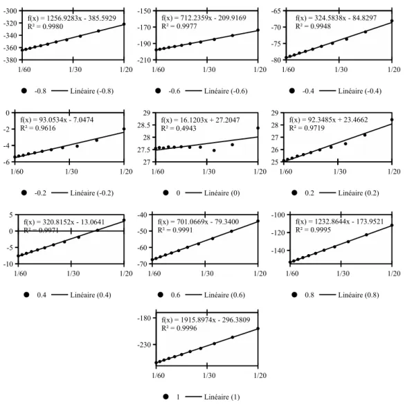
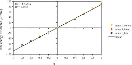
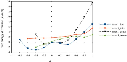
10.5.1 Box length dependance and charge dependance of free energy, 66 10.5.2 Comparison with IET after corrections, 69
10.5.3 Dependence on mmax and nmax, 70
10.6 Uncharged LJ centers, 73 10.7 Linear solutes, 74 10.8 First conclusion, 75
11 computing performance
77
11.1 FFT, 77 11.2 FGSHT, 78 11.3 k-kernel, 7911.4 Entire iteration of Fexc evaluation, 80
11.4.1 “naive” methods and “convolution_pure_angular”, 80
11.4.2 “convolution_standard” and “convolution_pure_angular”, 81 11.4.3 “convolution_standard” and “convolution_asymm”, 81 11.4.4 Distinction of mmax and nmax, 82
11.5 Global view of the code performance, 82
iv applications 83
12 comparison to md simulation
85
12.1 LJ centers, 85
12.2 Charged CH4 series, 86
12.3 Solvation free energy of single ions, 86 12.4 Small molecules, 88
v conclusion and perspectives 95
13 conclusion
97
14 perspectives
99
14.1 Reduce memory footprint in MDFT, 99 14.2 Site-based grid, 99
14.3 Theories beyond the HRF approximation and other improvements, 99 14.4 MDFT Viewer, 100
14.5 Application to real biological systems, and entropy, 100
vi appendix 101
viii contents
b
direct correlation function of water
104
b.1 Dipole DCF from molecular dynamics simulation, 104 b.2 DCF projections from bulk Monte Carlo simulation, 105 b.3 Comparison between DCFs, 105
c
error evaluation of interpolation strategies
for dcf in local frame
107
d
angular convolution using blum’s reduction
109
e
equivalence of quadrature-projection order
112
e.1 Gaussian quadrature, 112
e.2 Angular integration in GSHT, 112
f
rotational invariant expansion
114
f.1 Orthogonality of Φ, 114
f.2 Rotational invariance of Φ, 115 f.3 Transform in local frame, 116 f.4 Transform in fixed frame, 118 f.5 Symmetry, 119
f.5.1 Symmetric rules of F(ω1, ω2) in intermolecular form, 119
f.5.2 Symmetric rules of rotational invariant projections, 119
g
calculation of rotation matrix elements R
mµµÕ
by recurrence
121
g.1 Case of mmaxÆ 1, 121
g.2 Case of mmax>1, 122
h
properties of wigner 3j-symbol and gsh
124
h.1 Properties of Wigner 3j-Symbol, 124 h.2 Properties of GSH, 125
h.3 Convention of GSH, 126
List of Figures
Figure 1.1 The solvation process, 2 Figure 2.1 Continuum solvent model, 7 Figure 2.2 Definition of cavity surfaces, 8 Figure 2.3 Euler angles, 11
Figure 2.4 LJ pair potential, 12 Figure 2.5 Water models, 13
Figure 2.6 Interactions in a flexible model, 14 Figure 2.7 Hierarchy of solute models, 15
Figure 4.1 Solute charge density projected onto grids, 23 Figure 5.1 Main structure of code MDFT, 29
Figure 6.1 Molecules 1 and 2 in different coordinate systems, 33 Figure 6.2 Rotation matrices, 34
Figure 6.3 Rotation to k-frame, 34 Figure 6.4 φ1≠ φ2 distribution, 36
Figure 7.1 Indices arrangement in a complete forward-backward FFT-2D pro-cess of m’◊m elements, 43
Figure 7.2 Commutativity of operations, 44
Figure 7.3 Distribution of points to be calculated according to symmetry in a 2D plan, 46
Figure 8.1 IQ model and summation scheme, 48
Figure 9.1 Process “find equilibrium density” in MDFT, 53 Figure 9.2 Possible algorithms for γ evaluation, 53
Figure 10.1 RDF with different resolution parameter, 57
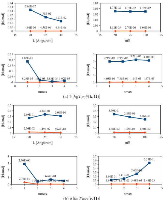
Figure 10.2 The minimum value of ∆ρ(r, Ω)/ρ0after a forward-backwardGSHT
process, 60 Figure 10.3 ρ0nl0‹ (r)and γ0nl
0‹ (r)of an artificial charged LJ center CH+40.4, 61
Figure 10.4 A k-kernel, 62 Figure 10.5 k-border effect, 63
Figure 10.6 Absolute differences in ˆγ(k, Ω) and γ(r, Ω), 64 Figure 10.7 Comparison of projections γ0nl
0‹ (r) for branches “naive_standard”
and “convolution_standard”, 65
Figure 10.8 Space-grid and Ψ dependence of code MDFT, 65
Figure 10.9 Original free energy of charged CH4, “naive_nmax1”, 67
Figure 10.10 Original free energy of charged CH4, “naive_interpolation” with
DCF of nmax =5, 68
Figure 10.11 Original free energy of charged CH4, “convolution_standard” with
DCF of nmax =1, 68
Figure 10.12 Quadratic charge dependence of free energy in CHq
4 series, 69
Figure 10.13 Free energy of charged CH4 compared to IET, without P-scheme
correction, 69
Figure 10.14 Free energy difference of CHq
4 series compared to IET, with all
corrections, 70 Figure 10.15 Free energy of CHq
4 series, with all corrections, 70
Figure 10.16 Free energy of CHq
4 series (with corrections) for different nmax
(mmax=5), 71
Figure 10.17 The projections ρ0nl
0‹(r)of some selected charges of CHq4 series
com-paring toIET, 72
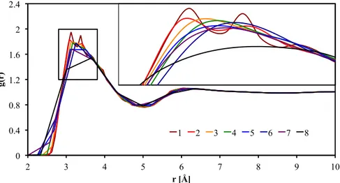
Figure 10.18 RDFandRPFof some selected charges of CHq
4 series with different
mmax and nmax, 73
Figure 10.19 Test linear solutes, 74 Figure 10.20 The projections ρmnl
µ‹ (r)of CO2 comparing toIET, 75
Figure 11.1 Timing of FFT for real-to-complex and complex-to-complex pro-cesses with respect to grid number N, 77
Figure 11.2 Timing of real-to-complexFFTprocesses with respect to its complex-to-complex process of the same grid number N, 78
Figure 11.3 Computing time ofGSHTand FGSHT, 78
Figure 11.4 Timing of real-to-complex FGSHT processes with respect to its complex-to-complex process of the same mmax and nmax, 79
Figure 11.5 Timing of a k-kernel, 79
Figure 11.6 Entire iteration of Fexc evaluation, 80
Figure 11.7 Performance comparison of “convolution_standard” and “convo-lution_pure_angular”, 81
Figure 11.8 Performance comparison of “convolution_standard” and “convo-lution_asymm”, 81
Figure 11.9 Performance comparison of “convolution_standard” for mmax =
nmax and mmax =5, 82
Figure 11.10 Timing of the whole F iteration, 82
Figure 12.1 RDF of rare gases compared to MD result, 85
Figure 12.2 RDF of charged CH4 series compared toMD result, 86
Figure 12.3 Test solutes, 89
Figure 12.4 Site-ORDF of test solutes, 91
Figure 12.5 Volume slice of solvent number density n(r)for pyrimidine, 94 Figure 12.6 Iso-surface of solvent number density n(r) = 2.4 for test water
molecules, 94
Figure 14.1 Site-site grid model, 100 Figure A.1 Function growth, 103
Figure B.1 Comparison between DCFprojections, 106
Figure C.1 Error of finding ˆc(k, Ω1, Ω2)by interpolation, 108 Figure F.1 Symmetry operations of a 2-molecule system, 119
List of Tables
Table 1.1 Solvation theories, 3
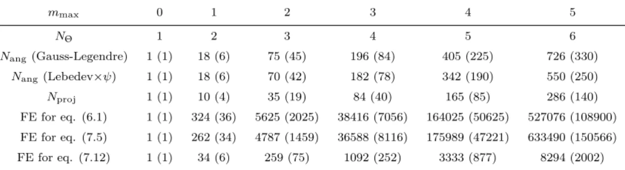
Table 2.1 Structural parameters of SPC and SPC/E water, 14 Table 7.1 Number of FE needed by OZ equation of different form, 40 Table 9.1 Branch option in MDFT, 54
Table 10.1 Minimized free energy given by different convergence criteria, 56 Table 10.2 Maximum absolute error Emax
a of some function f(Ω)introduced by a forward-backward GSHT process, 59
Table 10.3 Minimized free energy via different branches MDFT, 60
Table 10.4 Parameters of charged CH4 LJ centers for test usage, 66
Table 10.5 Methods and parameters for charged CH4 series test, 66
Table 10.6 Free energy of CHq
4 series (with corrections) for different mmaxand
nmax, 71
Table 10.7 Free energy of rare gases, 74 Table 10.8 Parameters of test solutes, 74 Table 10.9 Free energy of solutes, 75 Table 11.1 Timing of loop k, 80
Table 12.1 Free energy and first maximum of ion-water oxygenRDFfor alkali and halide ions from experimental andMDsimulation results, 87 Table 12.2 Free energies and first RDF maximum of single ions from MDFT
results, 87
Table 12.3 Parameters of test solutes, 90
Notations
Ω Grand potential [kJ · mol≠1]
Ξ Grand partition function, dimensionless F Helmholtz free energy [kJ · mol≠1]
F[ρ] Solvation free energy functional [kJ · mol≠1]
ρ(r, Ω) Density variable of solvent [Å≠3]
Ω Orientation variable in laboratory coordinate system, Ω ©(Θ, Φ, Ψ)
ω Orientation variable in intermolecular coordinate system, ω ©(θ, φ, ψ)
n(r) Number density of solvent [Å≠3], n(r) =s dΩρ(r, Ω)
ρ0 Bulk solvent angular density, n0 = (s dΩ)ρ0 is the bulk solvent number
density, both of unity [Å≠3]; in this thesis, n0 =0.0332891 is used as given
by the original code
Fid[ρ] Ideal free energy functional [kJ · mol≠1]
Fext[ρ] External free energy functional [kJ · mol≠1]
Vext External potential imposed by the solute [kJ · mol≠1] µ Chemical potential of unity [kJ · mol≠1]
Fexc[ρ] Excess free energy functional [kJ · mol≠1]
γ Normalized gradient of excess free energy functional, dimensionless g Pair distribution function (PDF), dimensionless
h Pair correlation function (PCF), or total correlation function (TCF) in
certain references, dimensionless
c Direct correlation function (DCF), dimensionless RmµÕµ Generalized spherical harmonics (GSH)
Φmnlµu Rotational invariant bases defined in appendix F
P Polarization [Å≠3]
qe Elementary charge, qe =1.602176565 · 10≠19[C]
q Charge of unity [C]; q=q/qe is the number charge, dimensionless
ε0 Vacuum permittivity, ε0 =8.854187817 · 10≠12[C2· J≠1· m≠1]
ε Dielectric constant (relative permittivity) of solvent, dimensionless NA Avogadro constant, NA=6.02214129 · 1023[mol≠1]
fQ fQ =qe210≠3NA/(4πε010≠10), electrostatic potential unit so that fQ· q2/ris in [kJ · mol≠1], where q is the number charge without unity, r in [Å]
KB Boltzmann constant, KB =1.3806488 · 10≠23[J · K≠1]
β β = (KBT)≠1, reciprocal of the thermodynamic temperature [mol · kJ≠1]
Acronyms
DCF direct correlation function
DFT discret Fourier transform, also refers to density functional theory
FE function evaluation
FFT fast Fourier transform
FGSHT fast generalized spherical harmonic transform
GSH generalized spherical harmonic
GSHT generalized spherical harmonic transform
HNC hypernetted-chain (approximation)
HRF homogeneous reference fluid (approximation)
IET integral equation theory
MC Monte Carlo
MD molecular dynamics
MDFT molecular density functional theory
MOZ molecular Ornstein-Zernike (equation)
MRSO molecule rotation symmetry order, s=1 or 2 according to symmetry axis
OZ Ornstein-Zernike (equation)
PCF pair correlation function
PDF pair distribution function
QM quantum mechanics
RDF radial distribution function
RPF radial polarization function
1
Introduction
This thesis aims to develop an original numerical toolkit for physical chemists and struc-tural biologists based on the molecular density functional theory (MDFT), which makes it possible to predict the solvation properties of arbitrary molecular objects in arbitrary molecular solvents (mainly water) efficiently and with microscopic accuracy. The intro-duction will seek to highlight the objective of this thesis and help explain such topics as why theorists are interested in the nature of solvation, what are the present computing trends in solvation simulations, and where our work situates in this frame of solvation theories.
1.1
modeling of solvent effectsSolvation is a fundamental phenomenon in chemistry. The chemical behavior of numer-ous systems strongly depends on the nature of solvation; for example, this is the case for the reaction mechanisms in metal-organic reacting centers [1, 2], or pharmaceutical studies [3–5]. The solvation properties demanded by scientific studies are highly diverse; they include the free energy of solvation, solubility, concentration, partition coefficient, saturated vapor pressure, pH value, the 3D solvation structure, etc. Overall, interest in these solvation properties touches many fields of study such as chemistry and biochem-istry, as well as pharmaceutical, environmental, and agrochemical industries. Unlike the well-studied quantum mechanics (QM) for chemical interactions at a microscopic scale, and the finite element models for macroscopic physical processes, the theories of solvation lie in-between these description scales and are still under development, owing to the am-biguous compromise between accuracy and computing cost, and the rapid development of computer hardware which makes complicated calculations more and more accessible. In a word, the studies in this domain are quite vibrant.
To change a phenomenon into a model, we must first understand its process. Solvation is defined as the process of moving a molecule from the gas phase (or vacuum) to a condensed phase (figure 1.1), which builds a stabilizing interaction with the solute (or solute moiety, e.g., residues, interfaces, etc.) [6]. Such interactions are mostly classical interactions, involving electrostatic and van der Waals forces; but there are also additional specific chemical effects such as hydrogen bond formation, and quantum effects for some small solvent molecules whose vibrational or rotational energy states are at the same magnitude as kBT, as well as other effects, etc.
As not all kinds of interactions are important in applications, different models and methods have been developed according to the usage.
For most of the 20th century, the study of solvation effects has been dominated by continuum (implicit) models [7, 8], which mostly rely on the continuum dielectric de-scription of the solvent and are not costly in terms of computation resources. They provide an accurate way to treat the strong, long-range electrostatic interactions which dominate many solvation phenomena, but lack detailed information on the first solvation shell. This information mainly includes the cavity formation energy and solute-solvent van der Waals interactions, which are often roughly treated by introducing an artificial form of cavity that links to the form of the solute. The methods for testing electrostatic
1.2 scope of this thesis 3
model (RISM), which discretizes the distribution and correlation functions into site-site functions, and solves somewhat phenomenologicalOZ and closure equations in a matrix form [15]. On the other hand, Blum [16–18], Fries and Patey [19] extend theOZequation into a full molecular form, where the distribution and correlation functions depend on both position and orientation. In their theory, the orientation part ofOZequation is simplified by expanding the distribution and correlation functions onto rotational invariants, which can be expressed in terms of Wigner generalized spherical harmonics.
The classical density functional theory approach deals with inhomogeneous liquids, and uses the same variation principle and minimization strategy [20–22] as electronic density functional theory (eDFT) for electron-electron interactions. The latter has received im-mense success in computational chemistry. ClassicalDFT gives the solvation free energy of the grand potential (usually named as free energy for simplification) and the equilib-rium solvent density by minimizing the free energy functional of the solvent density in the presence of a given external potential. Borgis and collaborators [23–32] have recently gen-eralized it into the molecular case, leading to molecular density functional theory (MDFT), where the solvent density depends on both position and orientation, ρ(r, Ω). The main theoretical difficulty lies in the definition of well-funded and reliable functionals of the ex-cess free energy Fexc[ρ], accounting for the geometric complexity of the solvent molecule.
Some recent research has shown that MDFT is capable of describing linear solvents like acetonitrile, but still has some caveats for the most complex solvent, water [32]. MDFT
can be proven as mathematically equivalent to the two-component molecularIET, in the limit that the functional is continuous (grid infinitely fine) and in an infinite system.
The majority of work of all these theories has been focused on water, since it is one of the most difficult systems to model due to its molecular geometry, unavoidable multi-body character, quantum effects, and hydrogen bonds, to name a few. The importance of including instantaneous polarization in potential functions is also an issue [33, 34]. However, since polarizable force fields are not yet in common use, the simulations by micro-states and the liquid theory which feed on force fields also have their own limits, compared to the continuum model which can be totally polarizable. The advantages and disadvantages of each branch of theory are listed in table 1.1.
theory speed long-range first-shell polarizable solvent
Continuum model fast yes no fully
Classical molecular simulations costly yes yes partially, very costly Theory of liquids fast yes yes partially
Table 1.1: Solvation theories
1.2
scope of this thesisThis thesis aims at developing the theory and the code of MDFT, focusing on the gener-alization and algorithmic acceleration of the excess free energy functional Fexc evaluation
under homogenous reference fluid (HRF) approximation, which will be discussed in detail in later chapters.
Chapter I reviews a selection of models and methods to describe solvent effects. It includes the implicit and explicit models, the basics of liquid-state theory, as well as its two frontier research domains,MDFTandIET. Some details of the codeMDFT, associated to the MDFT approach, on which all the developments of this thesis are based, are also included.
4 introduction
Chapter II presents all the theory developed and newly used in this thesis. Two algo-rithms for the excess energy functional evaluation underHRFapproximation are proposed. One is an extension of the previous algorithm which could be applied to only linear sol-vents (or linearized molecular solsol-vents), to a full 3D molecular solvent case; while the other is a new algorithm that integrates the molecular OZ equation treatment of angu-lar convolution into MDFT. The solvation properties that the code generates are also presented, mainly containing the corrections of free energy and solvent structure profiles.
Chapter III reports all the implementation results, which are divided into two aspects: the “accuracy”, which involves the error evaluations, comparisons between algorithms, and withIET results; and the “performance”, which evaluates the computing cost, from the parts of the code to the entire branches.
Chapter IV gives applications to some LJ centers, ions and small molecules. Some works that remain unachieved are put in the perspectives.
Chapter I
State of the Art: Solvation, Models
and Methods
This chapter gives a brief review of all the basic concepts and previous work that this thesis is based on.
In section 2, we begin by introducing the frequent models of solvent in a simulation, from the simplest implicit continuum model to the most complex explicit one. The overview of these models then helps to understand the choice of description scale used in our study, as well as its limits.
Once the model is chosen, all the theories become mathematical problems. Section 3 reviews some basic concepts of statistical mechanics for liquids (i.e. theory of liquids), which present some brief formalisms deduced for an atomic solvent model. Two frontier approaches are introduced with a few deductions: the classical density functional theory (cDFT), and the integral equation the-ory (IET). A mathematical equivalence between these two theories is also presented.
The following section 4 gives the extension of the two theories to the molecular solvent case, i.e. the molecular density functional theory (MDFT) that this thesis works upon, and the molecular Ornstein-Zernike (MOZ) approach for
IET. The equivalence between these two theories gave us the idea to use the expansion techniques inIET to serveMDFT.
Section 5 gives some supplementary presentation of the initial code MDFT, which the development of this thesis is based on.
8 model of solution system
which polarizes the medium, and the action back of the medium on the molecule (reaction field).
The initial two terms in eq. (2.1) are linked to the configuration of the first solvation shell (cavity). The definition of cavity varies from the simplest sphere or ellipsoid to the ensemble of atomic surfaces defined by the van der Waals radii in the solute. It is somewhat reasonable to consider the cavity area as proportional to the number of solvent molecules in the first solvation shell. This number can be calculated as the area passing through the middle region of first shell solvent. This area, named the solvent-accessible surface area (SASA) [36, 37], can be calculated by adding the radius of the probe solvent ball to the solvent excluded surface area (figure 2.2).
Van der Waals surface solvent-accessible surface (SAS) solvent excluded surface (SES) probe sphere
Figure 2.2: Definition of cavity surfaces. The solvent accessible surface (SAS) traced out by the center of the probe representing a solvent molecule. The solvent excluded surface (SES) is the topological boundary of the union of all possible probes that do not overlap with the molecule.
The energy required to create such a cavity and the stabilization due to van der Waals interactions between the solute and solvent, assumed to be proportional to the surface area of the cavity, is expressed as
∆Gcavity+∆Gdispersion=γSSASA+β (2.2)
or parameterized by having a constant ξ specific for each atom type, with the ξ parameters being determined by fitting to experimental solvation data:
∆Gcavity+∆Gdispersion= atoms
ÿ i
ξiSi (2.3)
The models and methods employed to calculate the electrostatic contribution ∆Gelec
have varied greatly according to their usage. The sections below list the most common examples. On another topic, the integration of continuum models into QM calculations is also a very important field; these developments will not be detailed here as they do not connect yet to our work. Such kinds of methods are called the self-consistent reaction field (SCRF) models, which integrate the calculation of the solute-solvent interaction in addition to that of the solute wave function by an iterative procedure. Some examples are presented in the list of Gaussian keyword SCRF [38], and the field is well reviewed by, for example, Tomasi [9, 10] and Jensen [7].
2.1.1 Poisson-Boltzmann methods
The Poisson-Boltzmann equation (PBE) [39] makes it possible to calculate the position-dependent electrostatic potential Velec(r)in the continuum model, such that the
electro-static component of the free energy can be written as ∆Gelec = 1
2
⁄
2.1 continuum solvation models 9
where ρq is the charge distribution of the solute.
The Maxwell-Gauss equation in SI units convention gives
Ò · D(r) = ρq(r)
ε0 (2.5)
where D(r) = ε0E(r) +P(r) is the electric displacement field, P(r) is the system po-larization, E(r) the electric field, and ε0 the vacuum permittivity. D(r) can also be
expressed in terms of the position-dependent dielectric constant ε(r), D(r) = ε(r)E(r), which thus gives
Ò · ε(r)E(r) = ρq(r)
ε0 (2.6)
or in terms of electrostatic potential:
Ò ·[ε(r)ÒVelec(r)] =≠ρqε(r)
0 (2.7)
This second-order differential equation (2.7) is called the Poisson equation.
This equation cannot be solved analytically for complex geometries (such as a protein). Therefore it is done numerically using appropriate methods; for example, as mentioned in the article of Roux and Simonson [40] or Holst [39]. A density functional approach based on the minimization of the polarization density can also be used to solve this equation [41, 42].
If the solvent is ionic, the Poisson equation can be modified by taking into account a (thermal) Boltzmann distribution of ions in the solvent, i.e.,
ρtot(r) =ρq(r)≠ 2qnionsinh(kq
BTVelec(r)) (2.8)
for a salt composed of ions of charge +q and ≠q and of density nion. Replacing in eq.
(2.7) leads to the Poisson-Boltzmann Equation:
Ò ·(ε(r)ÒVelec(r))≠2qnion ε0 sinh 3qV elec(r) kBT 4 =≠ρ(r) ε0 (2.9)
2.1.2 Born / Onsager / Generalized Born models
For simple geometries, the Poisson equation (2.7) can be solved analytically. The simplest model is a spherical cavity. For a net charge q in a cavity of radius a, the electrostatic free energy of a medium with a dielectric constant of ε is given by the Born formula:
∆Gelec(q) =≠ 1 8πε0 3 1 ≠1ε 4 q2 2a (2.10)
Other similar models include the Onsager model, in which a point dipole (characterized by the dipole moment µ) is put in a spherical cavity. The Kirkwood model refers to a general multipole expansion in a spherical cavity, while the Kirkwood-Westheimer model arises for an ellipsoidal cavity. Those simplified models are not fully able to predict the solvent behavior in many realistic cases [7].
The generalized Born (GB) model is an empirical model based on the superposition of several net charges in spherical cavities as the Born model describes, with a similar formula: ∆Gelec =≠ 1 8πε0 3 1 ≠1ε 4 ÿ i ÿ j qiqj fij (2.11)
10 model of solution system
where the function fij depends on the internuclear distance rij between the centers of atoms i and j and on the Born radii for each pair of atoms ai and aj:
fij = ˆ ı ı Ùr2 ij≠ aiajexp A r2ij 4aiaj B (2.12)
The key (empirical) point is to be able to attribute an effective Born radius ai to each atom inside the complex, non-spherical cavity formed by the solute. Once this is accom-plished, the GB model provides a very fast method, with an overall accuracy comparable to that of Poisson-Boltzmann calculations. That makes it widely used in computational structural biology to perform structure optimization and molecular dynamics simulations.
2.2
model potential of explicit moleculesThe model potential frequently used in the theory of liquids is a classical, rigid, pairwise additive model [12, 13]. It is based on three assumptions.
1. Firstly, the quantum effects should be ignored. It is assumed that the rotational and transitional motion of solvent particles are continuous and classical, which means the separation of both transitional and rotational states are largely inferior of kBT.
For light molecules, that is not always convincing. Some molecules containing hy-drogen (e.g. H2O, NH3, and particularly H2) exhibit obvious quantum effects at low
temperatures in the liquid state. Gaseous H2O and NH3 also need quantum effect
corrections. However, for the liquid of most interest to us, H2O at room
tempera-ture, the contribution of this effect is small enough to be neglected. And obviously, there should not be any chemical interaction of the solvent with the solute.
2. Secondly, the intramolecular movement (vibration and internal rotation) should
Compared to atomic models that only depend on rN, the angular correlations can give influence on both structural and thermodynamic proprieties. That is why our theory is extended to linear case,
Ω ≡(Θ, Φ), then molecular case,
Ω ≡(Θ, Φ, Ψ).
be either independent of transitional and rotational movement or absent. This rigid molecule approximation assumes that the intermolecular potential U(rN, ΩN)
for N particles only depends on the positions of the N molecular centers rN ©
(r1, r2, . . . , rN) and on their orientations ΩN © (Ω1, Ω2,· · · , ΩN), where Ω ©
(Θ, Φ, Ψ)represents the Euler angles (figure 2.3). The natural choice for the
molec-ular center is the center of mass. This is, however, arbitrary if only equilibrium properties are considered.
The rigid approximation is quite realistic for molecules in which the separation of vibrational states largely exceeds kBT, implying that the molecule stays in its
ground vibrational state. This is the case for many small solvent molecules such as N2, CO2, C6H6, and indeed for the bending and stretching modes of water.
3. Finally, the intermolecular forces have to be assumed as pairwise additive: U(rN, ΩN) = 1 2 ÿ i”=j u(rij, Ωi, Ωj) = ÿ i<j u(rij, Ωi, Ωj) (2.13) This means that the model potential only depends on the intermolecular separation
rand on the molecular orientations Ω1 and Ω2. This approximation is quasi-exact
for low density gases, where the contribution of the three and more body terms decreases rapidly. But for dense fluids, in most of the cases the multi-body potential cannot be ignored. The complete model potential with higher-order corrections can be written in the form of
U(rN, ΩN) =ÿ i<j u(ij) + ÿ i<j<k u(ijk) + ÿ i<j<k<l u(ijkl) +... (2.14)
2.2 model potential of explicit molecules 11
Figure 2.3: Euler angles. The basis vectors of the new orientation are obtained by 3 sequential operations: (1) A rotation φ(0 < φ < 2π)about the z-axis, bringing the frame of axes from the initial position S into the position SÕ(2) A rotation θ (0 < θ < π)about the
y-axis of the frame SÕ, which is transformed into SÕÕ (3) A rotation ψ (0 < ψ < 2π)
about the z-axis of the frame SÕÕ.
where u(ij) = u(rij, Ωi, Ωj) and u(ijk) = u(rij, rjk, rki, Ωi, Ωj, Ωk), etc. The omission of the three-body and higher-order terms can cause errors, for example, in surface tension and surface energy calculation [43]. However the higher order terms are often accounted for by an effective pair potential (measured by experiments or calculated by simulations), which reduces considerably the computational cost for simulations, or the degree of theory needed. Such models are presented below, going from simple to molecular liquids. For the molecular solvent considered in this thesis, water, most publications have stayed at this two-body level of description.
2.2.1 Interaction of spherical particle
The simplest model of a fluid is the hard sphere model. With d the hard-sphere diameter, the pair potential is defined as:
u(r) = Y _ ] _ [ Πr < d 0 r > d (2.15)
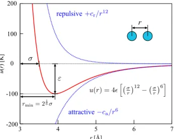
This model is indeed a fundamental reference model in statistical mechanics, and it can represent some physical systems, such as neutral colloidal suspensions [44]. However, the absence of attractive force, which precludes the existence of a liquid-gas transition, makes it too simple for realistic fluids. More realistic neutral particle models, like the Lenard-Jones (LJ) model, exhibit a potential energy curve that has the same shape as the real interaction of rare gas, as shown in figure 2.4.
The Lennard-Jones (LJ) interaction gives
uLJ(r) =4ε C3‡ r 412 ≠ 3‡ r 46D (2.16)
where r is the distance from centre to centre, ‡ is the collision diameter or the particles separation where u(r) =0, and ‘ is the well depth of the potential (of unity of energy). The well minimum occurs at rmin = 21/6‡ and u(rmin) = ≠‘. The parameters ‡ and ‘
12 model of solution system attractive r repulsive 200 100 0 -100 -2003 4 5 6 7 r [Å] u( r)[ K ]
Figure 2.4: LJ pair potential. The plot gives the potential energy u(r)versus internuclear distance r of two particles. At large distances, both attractive and repulsive interactions are small. As the distance between the atoms decreases, the attractive electron-proton interactions dominate, and the energy of the system decreases. At the observed bond distance, the repulsive electron-electron and proton-proton interactions just balance the attractive interactions, preventing a further decrease in the internuclear distance. At very short internuclear distances, the repulsive interactions dominate, making the system less stable than the isolated atoms.
Theoretically, all terms in the multipole series represent attractive contributions to the potential. The leading term, varying as r≠6, describes the quantum dipole-dipole
in-teraction. Higher-order terms represent dipole-quadrupole (r≠8), quadrupole-quadrupole
(r≠10) interactions, and so on, but these are negligible compared to r≠6. The short-range
interaction is difficult to define properly, and for the sake of simplicity and numerical efficiency, it is defined as r≠12 in the LJ model.
If the spherical particles are charged (as in molten salts), the electrostatic interaction between them is described by the Coulomb point charge interaction:
uCoul(r) = q1q2
4fiÁ0r (2.17)
For such charged simple fluids, the overall pair u(r) is a sum of LJ and Coulomb interactions. Such decomposition can be extended to molecular fluids in terms of site-site interactions, which are discussed in the following section.
2.2.2 Site-site interactions
Indeed, a spherical description of interactions is not sufficient to fully describe molecular fluids. The site-site model is a further extension of atomic models in which the solvent molecule is represented by a set of discrete interaction sites. The total potential energy is a sum of spherical interaction potentials:
u(1, 2) =ÿ
– ÿ
—
u–—(|r2—≠ r1–|) (2.18)
where risis the coordinates of site s in molecule i, u–—(r)the interatomic potential energy of pairs of sites – and —, as discussed above. More specifically, it is generally decomposed into a Lennard-Jones and a Coulombic contribution:
u(1, 2) =ÿ – ÿ — Y ] [4‘–— S U A ‡–— r–—12 B12 ≠ A ‡–— r–—12 B6T V + 1 4fiÁ0 q–q— r–—12 Z ^ \ (2.19)
14 model of solution system
modeled using Coulomb’s Law and the dispersion and repulsion forces using the Lennard-Jones potential, as described above.
With respect to the original SPC model, the SPC/E model takes into account the polarization in an implicit and phenomenological way, re-normalizing the dipole of the effective pair model, and thus increasing the partial charge slightly compared to SPC (table 2.1; the center of water molecule has been placed at atom O, for convenance). The SPC/E model gives a better radial distribution function and diffusion constant than the SPC model. It is the most commonly used model for applications.
It should be noted that any rigid solvent model is compatible with the theory that this thesis is based on, e.g. acetonitrile used in [32]. model ‡ [Å] Á[kJ · mol≠1] l 1 [Å] q1 [qe] q2 [qe] ◊ [°] SPC [48] 3.166 0.650 1.0000 +0.410 -0.8200 109.47 SPC/E [47] 3.166 0.650 1.0000 +0.4238 -0.8476 109.47 experiment [49] - - 0.991 - - 105.5
Table 2.1: Structural parameters of SPC and SPC/E water
2.2.5 Flexible and polarizable models
Up to this point, molecules were considered as rigid bodies. Flexible models give extra degrees of freedom in vibration and internal rotation. In that case, the interaction po-tential contains several extra terms, yielding typically five kinds of forces: three for the direct interactions in addition to the two indirect interactions (LJ and Coulomb).
stretch terms bend terms torsional terms non-bonded interactions
U= X bonds Kr(r − req)2+ X angles Kθ(θ − θeq)2+ X dihedrals Vn 2 [1 + cos(nφ − γ)] + X i<j " Aij r12 ij − Bij r6 ij + qiqj "rij # + − b θ φ r r
Figure 2.6: Interactions in a flexible model
The flexible yielding can deal with the non-rigidity of the solvent, which is partially polarized owing to the vibrational degrees of freedom (the so-called atomic polarizability). On the other hand, electronic polarizability (the deformation of the molecule electron cloud under the action of the external electric field) can be taken into account even in a rigid model. This polarizability can be described by introducing a modifiable charge distribution, for example by adding an induced dipole at the molecular center of the molecule, or even on each of its atomic sites, and by solving the set of induced dipoles self-consistently. Introducing variable atomic charges is possible too [50]. Optimizing the induced charges/dipoles has a large computational overhead compared to fixed charges.
Complex models require expensive computing cost, but still can have large fluctuations due to use of imposed small system size. There is a compromise between the choice of model and the choice of system size. For this reason, the rigid models are still the most popular nowadays. On the other hand, computing technologies have greatly developed compared to the theories themselves, which makes it possible to use more and more precise models in computation.
3
Statistical Mechanics of Atomic Fluids
Statistical mechanics serves to deduce thermodynamic quantities from the Hamiltonian of any given system. In this section, we present some basic formalism for a classical atom-like spherical solvent model in grand canonical ensemble (µ,V ,T ). Firstly, we introduce the relations between the statistical mechanics and thermodynamic quantities. Then we change the view to the structure of the solvent. The two theories we use in this thesis, here referred to as IET and cDFT, as well as their equivalency, are presented with brief derivations in the following content. The majority of this section is based on the book by Hansen & McDonald [12, 51], and the articles and notes of Evans [21, 52, 53]. A very detailed review is done by Wu et al. [54] to the same purpose, thus here we only introduce the concepts that will be useful to understand this thesis.
3.1
hamiltonian and ensemble propertiesOnce we define a spherical solvent model, of which the movement only depends on its position and momentum(r, p), the instantaneous state (phase point, micro-state) of an N-particle solvent system is specified by 3N coordinates rN © r
1, . . . , rN and 3N momenta
pN © p1, . . . , pN. The internal energy of particles in a system is characterized by its
Hamiltonian: HN(rN, pN) =KN(pN) +VN(rN) +VNext(rN) (3.1) where KN(pN) = N ÿ i=1 p2i
2m is the kinetic energy;
VN(rN) =
N ÿ i<j
u(|ri≠ rj|) +3 body+. . . is the interatomic potential energy U(rN);
VNext(rN) =
N ÿ i=1
Vext(ri)is the potential energy arising from the interaction of the particles with the external field (e.g. a solute).
The grand potential, characteristic thermodynamic state function for the grand canon-ical ensemble, which depends on the chemcanon-ical potential µ, the volume V and the temper-ature T , is linked with the statistical mechanics quantities with the relation:
œ(µ, V, T) =≠kBTln … (3.2) where … = Œ ÿ N=0 e—µN h3NN ! ⁄ drNdpNe≠—HN(rN,pN) (3.3) = Œ ÿ N=0 1 N ! ⁄ drNe≠—VN(rN) AN Ÿ i=1 e—Vint(ri) Λ3 B (3.4) 16
3.2 functional derivatives and distribution functions 17
is the grand partition function, with Λ = 12fi—¯h2/m2≠
1 2
the de Broglie thermal wave-length, and
Vint(ri) =µ≠ Vext(ri) (3.5) the intrinsic chemical potential.
We can also define the intrinsic free energy: N =sdr ¯n(r) is the number of particles in canonical ensemble, but the formulae (3.6) and (3.8) are also available for grand canonical ensemble. Fint = F≠ ⁄ dr ¯n(r)Vext(r) = œ+µN≠ ⁄ dr ¯n(r)Vext(r) = œ+ ⁄ dr ¯n(r)Vint(r) (3.6) where F is the Helmholtz free energy and
¯ n(r) =ÈÍ(r)Í= K N ÿ i=1 ”(r≠ r1) L (3.7)
is the density profile of instantaneous density Í(r)distribution at equilibrium. The differential form of Fint is
”Fint =≠S”T+
⁄
dr” ¯n(r)Vint(r) (3.8)
with S the entropy.
The internal energy of the solvent contains two contributions, one due to the kinetic energy of the particles, KN(pN), and the other linked to the interaction between particles,
VN(rN). When the fluid is a perfect gas, which means VN = 0, it can be easily derived from eq. (3.2-3.5) that Fint has the following expression:
Fid=kBT
⁄
dr ¯n(r)Ëln1Λ3n¯(r)2≠ 1È (3.9) When interactions between particles are accounted for, the total expression of Fint is:
Fint=Fid+Fexc (3.10)
and the form of Fexc will be detailed in later sections.
3.2
functional derivatives and distribution functionsThe structure of the solvent in the grand canonical ensemble can be characterized by its
n-particle density fl(n)(rn) = 1 … Œ ÿ N=n 1 (N≠ n)! ⁄ dr(N≠n)e≠—VN(rN) AN Ÿ i=1 e—Vint(ri) Λ3 B (3.11)
which means the probability to find n particles in a volume element drn. In particular, the probability to find one particle in a volume element is the solvent density fl(1)(r) =n¯(r),
that ⁄
fl(1)(r)dr=ÈNÍ (3.12)
where ÈNÍ is the ensemble average of the number of particles, that is to say the average number of particles at equilibrium. fl(n)(rn)becomes flnif the system is homogeneous. It can be proven that
”œ
”Vint(r) =≠fl
18 statistical mechanics of atomic fluids
The corresponding n-particle distribution function is defined as:
g(n)(rn) = fl
(n)(rn) rn
i=1fl(1)(ri)
(3.14)
such that g(n)(rn)æ 1 when all pairs of particles becomes sufficiently large. The two-particle pair distribution function (PDF), g(2)(r
1, r2), is one of the most
im-portant quantities in the theory of liquids. Its corresponding pair correlation function (PCF) is defined as:
h(2)(r1, r2) =g(2)(r1, r2)≠ 1 (3.15) which vanishes when |r1≠ r2| æ Œ.
If we define the density-density correlation function as:
For any ensemble.
H(2)(r1, r2) =fl(1)(r1)fl(1)(r2)h(2)(r1, r2) +fl(1)(r1)”(r1≠ r2) (3.16) which means the correlation [55] between the instantaneous fluctuation of particle density from its ensemble average, it can be proven that
”œ2 ”Vint(r1)”Vint(r2) =≠—H (2)(r 1, r2) =≠”fl (1)(r 1) ”Vint(r2) (3.17)
As an analogue, the direct correlation function (DCF) is defined as the derivative of the excess free energy functional Fexc[fl]:
c(1)(r) =≠”(—Fexc[fl (1)]) ”fl(1)(r) (3.18) c(2)(r1, r2) = ”c (1)(r 1) ”fl(1)(r 2) =≠ ”2(—Fexc[fl(1)]) ”fl(1)(r 1)”fl(1)(r2) = c(2)(r2, r1) (3.19) c(n)(r1, . . . , rn) = ”c(n≠1)(r1, . . . , rn≠1) ”fl(1)(r n) (3.20) According to the definition of Fint, as well as the expression of ”Fint in eq. (3.8):
—Vint(r) = —”Fint[fl (1)] ”fl(1)(r) =— ”Fid[fl(1)] ”fl(1)(r) +— ”Fexc[fl(1)] ”fl(1)(r) = ln1Λ3fl(1)(r)2≠ c(1)(r) (3.21) The functional derivative chain rule leads to
⁄ dr3”Vint(r1) ”fl(1)(r3)· ”fl(1)(r3) ”Vint(r2) = ⁄ dr3”Vint[fl (1)(r 1)] ”fl(1)(r3) · —H (2)(r 3, r2) = ⁄ dr3 C 1 fl(1)(r1) ”(r1≠ r3)≠ c(2)(r1, r3) D · H(2)(r3, r2) = ”(r1≠ r2) (3.22)
in addition to the definition of H in eq. (3.16) gives
h(2)(r1, r2) =c(2)(r1, r2) + ⁄ dr3 1 c(2)(r1, r3)fl(1)(r3)h(2)(r3, r2) 2 (3.23) which is called the Ornstein-Zernike (OZ) equation.
3.3 classical density functional theory 19
3.3
classical density functional theory The density functional theory is based on two theorems :1. For a given choice of VN, T and µ, the intrinsic free energy Fintis a unique functional
of the equilibrium one-particle density ¯n(r), expressed by Fint[n¯].
2. Let n(r) be some arbitrary one-particle microscopic density, and define the grand potential functional œ[n]as:
œ[n] =Fint[n]≠
⁄
drn(r)Vint(r) (3.24)
Then the variational principle states that
œ[n]Ø œ[n¯] (3.25)
with the equal sign takes at n(r) = n¯(r). The differentiation of eq. (3.24) with respect to n(r) gives ”œ[n] ”n(r) -n=n¯ = ”Fint[n] ”n(r) -n=n¯ ≠ Vint(r) =0 (3.26)
The fact that the right hand vanishes at equilibrium is agreed with eq. (3.8).
The solvation free energy functional F is defined as the difference between the grand Here the character F is used for “free-energy functional”; it is a free energy of grand ensemble, but differs from Helmholtz free energy F . However, it can be proven that all the free energies become the same when the fluctuations in N and V are negligible [56].
potential functional of the solution system œ[n] and of the correspondent reference bulk solvent at equilibrium œ[n¯0]:
F[n] =œ[n]≠ œ[n¯0] (3.27)
As the external potential is absent for bulk solvent, we define:
Fint[n] = F[n]≠ ⁄ drn(r)Vext(r) (3.28) = Fint[n]≠ Fint[n¯0]≠ µ ⁄ dr∆n(r) = kBT ⁄ drn(r)Ëln1Λ3n(r)2≠ 1È+Fexc[n(r)] (3.29) ≠kBT ⁄ dr ¯n0 Ë ln1Λ3n¯0 2 ≠ 1È≠ Fexc[n¯0]≠ µ ⁄ dr∆n(r) where ∆n(r) =n(r)≠ ¯n0.
If we write the external free energy Fexc[n(r)] in Taylor expansion around ¯n0:
Fexc[n] © Fexc[n¯0] + ⁄ dr ”Fexc[n] ”n(r) -n=n¯0 ∆n(r) +1 2 ⁄ dr1dr2 ” 2F exc[n] ”n(r1)”n(r2) -n=n¯0 ∆n(r1)∆n(r2) +O(∆n3) = Fexc[n¯0]≠ kBT ⁄ drc(01)(r)∆n(r) ≠kB2T ⁄ dr1dr2c0(2)(r1, r2)∆n(r1)∆n(r2) +O(∆n3) (3.30)
where c(0n)(r)is the corresponding bulkDCFat equilibrium defined in eq. (3.20). Accord-ing to eq. (3.21):
c(01)(r) =ln1Λ3n¯0
2
20 statistical mechanics of atomic fluids we can find Fint[n] = kBT ⁄ dr5n(r)ln3n(r) ¯ n0 4 ≠ n(r) +n¯0 6 (3.32) ≠kB2T ⁄ dr1dr2c(02)(r1, r2)∆n(r1)∆n(r2) +O(∆n3) Therefore, if we define: Fid[n] =kBT ⁄ dr 5 n(r)ln 3n(r) ¯ n0 4 ≠ n(r) +n¯0 6 (3.33) Fexc[n] =≠kB2T ⁄ dr1dr2c0(2)(r1, r2)∆n(r1)∆n(r2) +O(∆n3) (3.34) Fext[n] = ⁄ drn(r)Vext(r) (3.35)
the free energy functional can be written as:
F[n] =Fint+Fext =Fid+Fexc+Fext (3.36)
Up to this point a brilliant approach has been built, in that for a given choice VN,
T and µ, one can obtain the equilibrium density of solvent ¯n(r) by minimizing the free energy functional: ”F[n] ”n(r) -n=n¯ =0 (3.37)
Note that the two terms Fid[n]and Fext[n]are physically exact, while the excess term
Fexc[n], which can be rewritten as:
Fexc[n] =≠kB2T
⁄
dr1dr2C(r1, r2)∆n(r1)∆n(r2) (3.38)
depends on the exact correlation function C(r1, r2)which is a priori unknown.
If we ignore the three-body and higher order terms in eq. (3.34), C(r1, r2) becomes that of the homogeneous reference fluid, which only depends on the relative distance, i.e.
c(2)(r1, r2) =c(r12), so that
Fexc[n]ƒ ≠kB2T
⁄
dr1dr2c(r12)∆n(r1)∆n(r2) (3.39)
This was called the homogenous reference fluid (HRF) approximation. The generalization to a molecular, non-spherical solvent for which orientations matter is described in §4.
3.4
integral equation theorySimilar to the DFT approach which aims to find the equilibrium solvent density fl(1) = ¯
n and the free energy functional F, the integral equation theory (IET) can also give structural and energetic informations by solving a pair of integral equations of h(2)(r
1, r2)
and c(2)(r
1, r2) to find the pair distribution function g and the difference of correlation
functions “=h≠ c which is directly linked to the free energy. One of the relations for h
and c is the OZ equation shown as eq. (3.23). Note that in k-space eq. (3.23) can take advantage of the convolution properties to give a simple product relation:
3.5 equivalence between cdft and iet for a dilute solution system 21
The second relation is a closure equation, which can be deduced from eq. (3.37), giving the minimum density
fl(1)(r1) =fl(01)exp 3 ≠—Vext(r1) + ⁄ dr2∆fl(1)(r2)c(2)(r1, r2) +O(∆fl2) 4 (3.41)
which gives, for example, when O(∆fl2) = 0, one of the simplest closure equations, the hypernetted-chainHNC approximation:
g(1, 2) =1+h(1, 2) =exp[≠—u(1, 2) +h(1, 2)≠ c(1, 2)] (3.42) Here u corresponds to Vext in eq. (3.41) when the particles 1 and 2 are respectively the
solute and solvent.
The general form ofOZ closure is:
g(1, 2) =exp[≠—u(1, 2) +h(1, 2)≠ c(1, 2) +b(1, 2)] (3.43) where the b is the bridge function. Other closures are also possible, such as Percus-Yevick (PY) approximation (a linear expansion of the second exponential term in HNC) specifically for systems with short-range forces, or mean-spherical approximation (MSA) in the limit of low density.
3.5
equivalence between cdft and iet for a dilute solution system The generalization of theOZequation in eq. (3.23) to n components can be written ash‹µ(1, 2) =c‹µ(1, 2) +fl ÿ ⁄ x⁄ ⁄ h⁄µ(1, 3)c‹⁄(2, 3)d3 (3.44)
where x‹ =N‹/N is the number concentration of species ‹ œ[1, n].
For a two-component homogeneous solute-solvent mixture, where the solute (M) is infinitely diluted in the solvent (S) (xS æ 1), the coupledOZ relations are written as
hSS(1, 2) =cSS(1, 2) +fl ⁄ hSS(1, 3)cSS(2, 3)d3 (3.45) hSM(1, 2) =cSM(1, 2) +fl ⁄ hSS(1, 3)cSM(2, 3)d3 (3.46) hMS(1, 2) =cMS(1, 2) +fl ⁄ hMS(1, 3)cSS(2, 3)d3 (3.47) hMM(1, 2) =cMM(1, 2) +fl ⁄ hMS(1, 3)cSM(2, 3)d3 (3.48) Eq. (3.45) is the OZ equation for bulk solvent. Eqs. (3.46) and (3.47) describe the correlations between the solute and solvents, which are equivalent. From eq. (3.47) we can deduce eq. (3.34) for the DFT approach, if we impose O(∆fl3) = 0, i.e. the HNC approximation. And inIET, eq. (3.46) is normally used for two-component solution. Eq. (3.48) is rarely used. The difficulty to solve such equation lies in finding a proper closure
equation. As the approximations like HNC are already quantitatively far from sufficient to describe solute-solvent correlation, it becomes very bad for solute-solute.