Anisotropic ductile fracture of metal sheets : experimental investigation and constitutive modeling

Anisotropic Ductile Fracture of Metal Sheets:

Experimental Investigation and Constitutive Modeling

by

Meng Luo

B.S. Thermal Energy and Power Engineering,

ARCHIVES

Shanghai Jiaotong University, Shanghai, China (2004)

MASSACHUSETTS INSTffTUTE

M.S.

Mechanical Engineering

OFTECHNOLOGY

Tsinghua University, Beijing, China (2007)

JUN 2 8 2012

LIBRA RIE S

Submitted to the Department of Mechanical Engineering

in partial fulfillment of the requirements for the degree of

Doctor of Philosophy in Mechanical Engineering

at the

MASSACHUSETTS INSTITUTE OF TECHNOLOGY

June 2012

C Massachusetts Institute of Technology 2012. All rights reserved.

A uthor ... ... .. ..

--Department of Mhanical Engineering

r ,May 28, 2012

C ertified by ... .. ...----.

Tomasz Wierzbicki Professor of Applied Mechanics, Department of Mechanical Engineering

I , Thesis Supervisor

Certified by ...-- a . ... .. . .... ..

Dirk Mohr

CNRS Associ fessor, Eco olytechnique 0 0 esi'ssetrvisor Accepted by ... ..

...----David E. Hardt Chairman, Departmental Committee on Graduate Students

Anisotropic Ductile Fracture of Metal Sheets:

Experimental Investigation and Constitutive Modeling

Meng Luo

Submitted to the Department of Mechanical Engineering

on May 28, 2012 in partial fulfillment of the requirements for the degree of Doctor of Philosophy in Mechanical Engineering

Abstract

Anisotropic mechanical properties are common in plastically deformed or thermo-mechanically processed metallic materials, e.g. in rolled or extruded sheet. Among them, the anisotropy of large strain plastic deformation and ductile fracture under multi-axial loading is highly relevant to various industrial applications such as metal forming, impact failure of structures, etc. In this thesis, a comprehensive study of the plasticity and ductile fracture of anisotropic metal sheets is presented, covering experimental characterization, constitutive modeling and numerical implementation. On the basis of an extensive multi-axial experimental program, the anisotropic plasticity of the present aluminum alloy is modeled using a macroscopic phenomenological model and a polycrystalline plasticity model, respectively. The proposed phenomenological modeling makes use of a linear-transformation-based orthotropic yield function with pressure dependence, as well as a combined isotropic/kinematic hardening law, and is able to capture most features of the anisotropic plastic behavior under various multi-axial stress states with good accuracy and computational efficiency. At the same time, a physically-motivated self-consistent polycrystalline plasticity model is utilized to describe the texture-induced anisotropy and through-thickness heterogeneity of the present sheet material. A Reduced Texture Methodology (RTM) is developed to provide the computational efficiency needed for industrial applications. In additional to an accurate prediction of all macroscopic material behaviors, the polycrystalline model reveals that the development of the crystallographic texture is the underlying mechanism of plastic anisotropy and heterogeneity. The anisotropic ductile fracture of the present aluminum alloy extrusion is investigated using a hybrid experimental-numerical approach. The experimental results show a strong dependency of the strain to fracture on the material orientation with respect to the loading direction. A new non-associated anisotropic fracture model is proposed which makes use of a stress state dependent fracture locus and an anisotropic plastic strain measure obtained through the linear transformation of the plastic strain tensor. It is shown that the use of the Modified Mohr-Coulomb (MMC) stress state weighting function in this anisotropic fracture modeling framework provides accurate predictions of the onset of fracture for all fourteen distinct fracture experiments. The proposed plasticity and fracture modeling framework is successfully validated on a industrial stretch-bending operation. Thesis Supervisor: Tomasz Wierzbicki

Title: Professor of Applied Mechanics Thesis Supervisor: Dirk Mohr

Acknowledgements

First of all, I would like to express my most sincere gratitude to my advisor, Professor Tomasz Wierzibicki, for his continuous support and guidance throughout my five years at MIT in his Impact and Crashworthiness Lab (ICL). I really appreciate the freedom and trust he offered me to shape this thesis from my own vision, as well as countless fruitful discussions between us. Many thanks are due to my co-advisor, Professor Dirk Mohr, for his insightful suggestions and valuable feedbacks, which have played a crucial rule on my approaches to research. I am grateful to Professor Lallit Anand for many constructive comments on my research and his excellent teaching in the area of solid mechanics. I am also indebted to Professor Pedro Reis for his willingness to serve on my thesis committee and discuss my research.

Special thanks are due to Dr. Gilles Rousselier from MINES ParisTech of France. His profound knowledge in metal plasticity and fracture and enthusiasm for research helped me greatly in entering the field of polycrystalline plasticity. I am also grateful to Dr. Lars Greve from Volkwagen for numerous valuable discussions.

It has been a pleasant journey for me to work in the ICL at MIT. I benefited a lot from the help of and the interaction with all members of the ICL, especially Dr. Yuanli Bai, Dr. Yaning Li, Dr. Carey Walters, Dr. JongMin Shim, Dr. Allison Beese, Dr. Elham Sahraei Esfahani, Mr. Matthieu Dunand, Mr. Kai Wang, Mr. Stephane Marcadet, Ms. Kirki Kofiani, Mr. Evangelos Koutsolelos, as well as Sheila McNary and Barbara Smith.

The financial support of my work through the MIT AHSS (Advanced High Strength Steel) consortium and the ONR MURI project through a sub-grant to MIT from Stanford University is gratefully acknowledged.

And finally, I would like to express my deepest thanks to my family for their unconditional love and support - at distance and while visiting me here in Cambridge. In particular, I would like to thank my wife Likun Zhang for her love, patience and

encouragement during my PhD studies at MIT, and our daughter, Emma, who just came to this world one month ago, but already became my greatest motivation to keep up the

Contents

1. Introduction ...

28

1.1 Anisotropic metal plasticity ... 30

1.2 Ductile fracture with anisotropy... 32

1.3 T hesis outline ... . 34

1.4 List of published, submitted or in preparation with reference to respective chapters ... 3 8

2. Experimental characterization and phenomenological

modeling of anisotropic plasticity under multi-axial loading

...

41

2.1 Introduction ... . 4 1 2 .2 M aterial ... 44

2.3 Uniaxial tensile experiments ... 45

2.4 B iaxial experim ents... 48

2.4.1 Experimental procedure ... 48

2.4.2 Experimental program ... 50

2.4.3 Experimental results... 52

2.5 Plasticity model for plane stress condition... 55

2.5.1 M odel choice... 55

2.5.2 M odel calibration ... 57

2.6 Extended model for general stress states ... 65

2.7 Bauschinger and Strength-Differential (SD) effects ... 68

2.7.1 Compression-tension experiments ... 68

2.7.2 Combined isotropic/kinematic hardening ... 70

2.7.3 Pressure dependence of the flow stress... 74

2.8 Concluding rem arks ... 76

3. Polycrystalline plasticity modeling of anisotropic FCC metal

sheets using a Reduced Texture Methodology (RTM)... 79

3.1 Introduction ... . 79

3.2 Experim ental details... 83

3.2.1 M aterial... . . 83

3.2.2 Uniaxial tension (full thickness)... 85

3.2.3 Uniaxial tension (reduced-thickness)... 88

3.2.4 Uniaxial compression-tension experiments (full thickness)... 90

3.2.5 Shear and non-proportional loading (reduced-thickness)... 91

3.2.6 Pseudo-experimental data for uniaxial tension (full- and reduced-thickness) ... . 94

3.2.7 Punch experiment (full- and reduced-thickness) ... 94

3.3 C onstitutive m odel ... 96

3.3.1 N otations ... 96

3.3.2 Kinematics of finite strain... 96

3.3.3 Elastic constitutive equation ... 97

3.3.4 The self-consistent polycrystalline model ... 98

3.4 M odel param eter identification ... 102

3.4.1 M odel param eters... 102

3.4.2 C alibration procedure... 103

3.4.3 Calibration #1: Full-thickness model with hardening... 105

3.4.4 Calibration #2: full- and reduced-thickness models with isotropic slip system hardening ... 107

3.4.5 Calibration #3: full and reduced thickness models with combined isotropic-kinematic slip system hardening... 107

3.5 R esults and discussion... 109

3.5.1 Identified reduced textures... 109

3.5.2 U niaxial tension ... I11 3.5.3 Evaluation for non-proportional loading ... 112

3.5.4 Evaluation for sim ple shear ... 112

3.5.5 Punching of a sheet ... 113

3.6 C oncluding rem arks ... 115

4. Modeling of multi-axial plastic deformation with

Strength-Differential effect using a RTM-based polycrystalline model

...

118

4 .1 Introduction ... 118

4.2 Experim ental database ... 122

4.2.1 Uniaxial tension (full- and recudeced-thickness) ... 123

4.2.2 Uniaxial compression & compression-tension (full-thickness)... 125

4.2.3 Biaxial experiments under proportional loadings (Reduced-thick)... 126 4.2.4 Biaxial experiments under non-proportional loadings (Reduced-thick). 131

4.3 Constitutive m odeling ... 132

4.3.1 A hardening law for large strain behavior ... 133

4.3.2 A generalized approach to model history effect ... 135

4.4 M odel calibration ... 138

4.5 Results and discussions ... 142

4.5.1 Identified reduced textures... 142

4.5.2 Results for uniaxial tension... 146

4.5.3 Strength-differential effect... 149

4.5.4 Evaluation for m ulti-axial large strain deformation... 150

4.5.5 Evaluation for non-proportional loadings ... 151

4.6 Structural validations ... 154

4.6.1 Circular punch indentation... 154

4.6.2 3-pt bending of a strip ... 155

4.7 Concluding rem arks ... 159

5. Ductile fracture characterization and modeling of metal

sheets with transverse anisotropy (planar isotropy)... 162

5.1 Introduction ... 162

5.2 Plasticity... 165

5.2.1 Experim ental characterization ... 165

5.2.2 Phenomenological m odeling... 168

5.2.3 Validation of transversely anisotropic plasticity m odel... 170

5.3 M odeling of ductile fracture initiation for sheets... 173

5.3.1 Characterization of the stress state... 173

5.3.3 Damage evolution rule... 178

5.4 Experimental-numerical fracture calibration ... 179

5.4.1 Conventional fracture tests ... 180

5.4.2 Biaxial fracture tests on butterfly specimens ... 188

5.4.3 Calibration and validation of the MMC fracture locus... 191

5.5 Post-failure behavior ... 194

5.5.1 Post-failure softening of finite elements ... 194

5.5.2 Mesh regularization during softening ... 197

5.5.3 Numerical implementation and fracture simulations for AA6061 -T6.... 200

5.6 Concluding remarks ... 204

6. Experiments and modeling of anisotropic ductile fracture207

6 .1 Introduction ... 207

6.2 Fracture experiments ... 208

6 .2 .1 M aterial... 208

6.2.2 Tensile specimens with circular notches... 210

6.2.3 Tensile specimens with a central hole ... 212

6.2.4 Butterfly specimens subject to shear loading... 213

6.2.5 Circular punch experiment... 215

6.3 Stress-state and strain path prior to fracture... 217

6.3.1 Definition of the onset of fracture... 218

6.3.2 Details on the finite element models... 218

6.3.3 Simulation of notched tension ... 221

6.3.5 Simulation of a butterfly specimen subject to shear loading ... 227

6.3.6 Simulation of the circular punch indentation test ... 229

6.3.7 Summary: evolution of stress states and equivalent plastic strain... 231

6.4 Anisotropic fracture modeling ... 234

6.4.1 Associated anisotropic fracture model... 235

6.4.2 Non-associated anisotropic fracture model... 239

6.4.3 Implementation and Validations ... 242

6.5 Discussion ... 245

6.5.1 Fracture mechanism ... 245

6.5.2 Critical comment on the proposed anisotropic fracture model... 249

6.6 Concluding remarks ... 250

7.

Structural Application: Numerical failure analysis of the

stretch-bending operation...

253

7.1 Introduction ... 253

7.2 M aterial and plasticity... 255

7.2.1 M aterial... 255

7.2.2 Plasticity characterization ... 255

7.2.3 Plasticity validation... 258

7.3 Fracture modeling and calibration ... 260

7.4 Experimental procedures for Stretch-bending ... 263

7.5 Numerical modeling and validation ... 266

7.5.1 M odel description ... 267

7.5.2 Results and validations ... 269

7.6 Parametric study... 278

7.6.1 Effect of tension level ... 278

7.6.2 Effect of tooling friction ... 280

7.6.3 Effect of mesh size... 282

7.6.4 Effect of the fracture locus... 284

7.7 Concluding remarks ... 286

8. Summary and future directions...

289

8.1 Summary of main results ... 289

8.2 Suggestions for future studies ... 292

List of Figures

Fig. 1-1: Anisotropic ductile fracture observed in industrial forming tests. (a) 3 Marciniak

forming tests specimens of TRIP780 steel, where crack always runs along rolling direction; (b) hole-expansion experiments of a DP780 steel where cracks tend to open in transverse direction... 29

Fig. 2-1: Specimen preparation from the extruded profile in different material

orientations. ... . 44

Fig. 2-2: Schematic of the dogbone specimen geometry... 45

Fig. 2-3: Results from uniaxial tensile testing. (a) Engineering stress-strain curves along the rolling direction (red curves, three tests), the cross-rolling direction (blue

curve) and an intermediate direction, a = 450 (black curve); (b) Calculated and

measured r-ratio variations (black curves and solid dots, respectively); Calculated and measured yield stress (blue curves and solid squares,

respectively)... . . 47

Fig. 2-4: (a) Schematic of the dual actuator system; (b) Specimen geometry and the

definition of the biaxial loading angle

#.

... 48

Fig. 2-5: Visualization of the loading states in the 3-dimensional stress-space. The solid dots represent the intersection of the linear stress paths with a quadratic yield surface. The labels next to the data points denote the biaxial loading angle 0 while the point color corresponds to the specimen orientation a (see legend). The green dots correspond to uniaxial tension (UT). ... 51

Fig. 2-6: Results from biaxial testing. Normal stress-strain curves (upper row) and shear stress-strain curves (lower row). (a) and (c) rolling direction (black curves) and

cross rolling direction (blue curves); (b) and (d) a = +451 (black curves) and

a = - 45" (blue curves)... 53

Fig. 2-7: Yield locus for different amounts of plastic work 6. Results from tension

experiments (#3 > 00) are depicted by square solid dots, while triangular dots are

used for compression experiments (#3 < 00). The solid lines depict the

prediction of the Yld2000-2D yield criterion. Absolute stress values are used for com pressions. ... .. 54

Fig. 2-8: Plane stress yield envelope for T = 0. ... 59

Fig. 2-9: Model predictions for uniaxial tensile loading along 7 different specimen

orientations. (a) Engineering stress-strain curves; (b) Engineering strain along the width as a function of engineering axial strain. The experimental results are

Stress-strain curves are translated with respect to each other for clarity; the origin of each curve is indicated by thin vertical and horizontal lines... 62

Fig. 2-10: Model predictions for the biaxial testing. Normal stress-strain curves (upper

row) and shear stress-strain curves (lower row) for a = 0 and a = 900. The

solid lines depict the prediction of the Yld2000-2D yield criterion, while the experimental results are shown by dashed curves... 63

Fig. 2-11: Model predictions for the biaxial testing. Normal stress-strain curves (upper

row) and shear stress-strain curves (lower row) for a = +450 and a = -450.

The solid lines depict the prediction of the Yld2000-2D yield criterion, while the experimental results are shown by dashed curves... 64 Fig. 2-12: Specimen and apparatus for compression-tension experiments. (a) schematic

and dimensions of the compression-tension specimen; (b) photo of the anti-bucking device (Beese, 2011)... 69

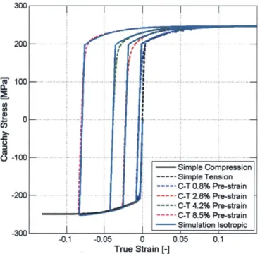
Fig. 2-13: Measured true stress strain curves. (a) compression followed by tension tests in TD; (b) comparison of uniaxial tension and uniaxial compression in TD. ... 70 Fig. 2-14: Measured and curve fitting of the isotropic, kinematic and total hardening in

the compression-tension tests along TD... 72

Fig. 2-15: Predictions of the stress strain curves for compression-tension tests in TD. (a) model with only isotropic hardening; (b) model with combined

isotropic/kinem atic hardening. ... 73

Fig. 2-16: Predictions of the stress strain curves for compression-tension tests along TD using a pressure dependent plasticity model. ... 76

Fig. 3-1: Grain orientations measured by EBSD. The dimensions are given in millimeter.

... 8 3

Fig. 3-2: Pole figures for (a,c,e) full-thickness specimens, (b,d,f) reduced-thickness specimens. The black dots represent experimental data (442 and 521 orientations, respectively). The colored dots represent the reduced texture models after calibration #3: 12-grain model of full-thickness specimen (left), 8-grain model of reduced-thickness specimen (right). First row (a-b): { 11

}

pole figures; second row (c-d): {I 10} pole figures; third row (e-f):

{

100} pole

figu es. ... . . 85

Fig. 3-3: True stress versus logarithmic strain curves for uniaxial tension. The dots show experimental data points for different specimen orientations while the lines show the corresponding 12-grain model results (after calibration #3)... 86 Fig. 3-4: Width versus thickness strain during monotonic uniaxial tension for different

specimen orientations: (a)-(b) results after calibration #1, (c)-(d) results after calibration #2. The experimental results are shown as open dots for the full thickness (FT) specimens and solid dots for the reduced thickness (RT)

sp ecim en s... . . 87

Fig. 3-5: Schematic of the reduced-thickness uniaxial tension specimen (the shape of the outer profile is identical to the full thickness specimen shown in Fig. 2-2... 88

Fig. 3-6: (a) Measured Lankford ratios (solid dots) with non-linear interpolation (stars),

(b) yield stress at 3% for specimens of full-thickness (red) and

reduced-thickness (blue). The two upper open dots at a = 900 correspond to

com pression tests... 89

Fig. 3-7: True stress versus logarithmic strain curves for compression followed by

tension. The dots show experimental data points while the lines show the model results (after calibration #3)... 90

Fig. 3-8: Shear stress versus shear strain (in machine coordinates) for a = 00 (ED parallel

to the y-axis of Fig. 2-4b) and o = 450 (ED rotated clockwise by 45' with

respect to the y-axis of Fig. 2-4b). The experimental results are shown by open dots while the corresponding simulation predictions (after calibration #3) are represented by solid lines. ... 92

Fig. 3-9: Loading paths of the non-proportional experiments on reduced-thickness specimens (a) in strain space and (b) in stress space; normal stress-strain curve and shear stress-strain curve for (c) experiment #1, and (d) experiment #2. The dots show the experimental results while the solid lines correspond to

predictions with the 8-grain model (after calibration #3)... 93

Fig. 3-10: Punch loading of disc specimens. (a) mechanical system, (b) contours of the maximum principal logarithmic strain as measured with stereo digital image

correlation and predicted by FEA (full-thickness), (c) force-displacement curve for full-thickness specimen, and (d) reduced thickness specimen, (e)

superposition of the numerically predicted cross-sectional shape (blue lines) with the full-thickness specimen at the onset of fracture. ... 96

Fig. 3-11: Crystal disorientation angles after calibration #3. (a) for 442 EBSD points for the full-thickness specimen, (b) for 521 EBSD data points for the reduced-thickness specimen; the EBSD measurements are compared with the three

components of the reduced texture of the 12-grain model (three colored curves in (a)) and the two components of the 8-grain model (two colored curves in (b)). The black curve shows the smallest disorientation for each data point... 110 Fig. 4-1: Results of the uniaxial testing program. (a) yield stress at 3% axial logarithmic

plastic strain of full- (red) and reduced-thickness (black) material, the two blue triangles represent full-thickness compression tests at a = 00 and 900; (b) measured width versus thickness strain curves during uniaxial tension for various m aterial orientations. ... 124 Fig. 4-2: Comparison of the stress-strain curves from full-thickness experiments and

12-grain numerical simulations with the new model with initial back stresses. (a) uniaxial compression and tension along ED; (b) uniaxial compression and tension along T D . ... 125

Fig. 4-3: Visualization of the loading states in the 3-dimensional stress-space. The solid dots represent the intersection of the linear stress paths with a quadratic yield surface. The labels next to the data points denote the biaxial loading angle

#

while the point color corresponds to the specimen orientation a and the type of experiment (see legend). The open dots with different shapes represent the

effecting zones of the five initial back stress components. (For interpretation of the references to color in this figure legend, the reader is referred to the web version of this thesis.)... 127

Fig. 4-4: Comparison between experimental data and model predictions of engineering stress-strain curves under proportional biaxial loadings: (a) shear stress-strain curves for pure shear loadings (3 = 00); (b) normal stress-strain curves under pure tension conditions (3 = 900); (c-f) results of all combined

tension/compression and shear loadings (00 < 3 < 900). Left (Right) column

contains shear (normal) stress-strain curves. (For interpretation of the references to color in this figure legend, the reader is referred to the web version of this

article.)... 13 0

Fig. 4-5: Comparison between measured and predicted (with a 8-grain model) shear engineering stress-strain curves for the large strain non-proportional experiment

(N P 3). ... 132

Fig. 4-6: Schematic of the five distinct pre-simulations for the identification of

standardized initial back stress components... 137

Fig. 4-7: { 11

}

Pole figures for (a) full-thickness specimens, (b) reduced-thickness specimens. The black dots represent experimental data (442 and 521 orientations, respectively). The colored dots represent the reduced texture models after calibration of the present model: 12-grain model of full-thickness specimen (left), 8-grain model of reduced-thickness specimen (right)... 143 Fig. 4-8: Comparison of the distribution of normalized resolved shear stresses of all slip

systems under simple tension between measured, reduced and isotropic texutre. (a)reduced texture with 12 grains; (b)reduced texture with 8 grains... 144 Fig. 4-9:

{111

} pole figure of the isotropic texture containing 500 grains... 146 Fig. 4-10: Stress strain curves during monotonic uniaxial tension for different specimen

orientations: (a)-(b) full-thickness specimens modeled with a 12-grain model, (c)-(d) reduced-thickness specimens modeled with an 8-grain model... 147 Fig. 4-11: Width versus thickness strain during monotonic uniaxial tension for different

specimen orientations. (a) full-thickness specimens modeled with a 12-grain model; (b) reduced-thickness specimens modeled with an 8-grain model... 148 Fig. 4-12: True stress versus logarithmic strain curves for compression followed by

tension. The dots show experimental data points while the lines show the predictions of the present model with initial back stresses. ... 149 Fig. 4-13: Experiment-simulation comparison of stress strain responses in the two small

strain non-proportional loading tests. (a) non-proportional loading test NP1; (b) non-proportional loading test N P2. ... 152

Fig. 4-14: Comparison between measured and predicted (using a Yld2000-3d phenomenological plasticity model with combined isotropic/kinematic hardening) shear engineering stress-strain curves for the large strain non-proportional experim ent (N P3)... 153

Fig. 4-15: Measured versus predicted force-displacement curves for punch loading of disc specimens. (a) full-thickness specimen; (b) reduced thickness specimen... 155 Fig. 4-16: 3-pt bending test. (a) mechanical testing system; (b) FE model... 156 Fig. 4-17: Comparison between measured and predicted (using the present RTM

polycrystalline model after calibration) force-displacement curves for the 3-pt bendin g tests. ... 157 Fig. 4-18: Comparison of the deformed specimen shape at different stages during the 3-pt bending tests. (a-c) test condition 1 with maximum punch depth of 15mm; (d-f) test condition 2 with maximum punch depth of 20mm. Red dotted frames represents the shape predicted by the FE model at the corresponding time.... 158 Fig. 5-1: Geometry of uniaxial tension specimens (dimensions in mm; specimen

thickness is 2mm). Specimens are cut at 00, 450, and 900 to the rolling direction.

... 16 6

Fig. 5-2: (a) Force versus displacement measured in uniaxial tensile tests (gauge length =

50.145 mm). (b) True stress versus plastic strain calculated up to necking... 167 Fig. 5-3: (a) Vertical and horizontal DIC "virtual" extensometers at their initial position.

(b) Transverse plastic strain versus through thickness plastic strain for uniaxial

ten sio n ... 167

Fig. 5-4: Swift law (power law) fitting of the isotropic hardening of AA6061-T6... 170 Fig. 5-5: Specimens of the biaxial plasticity testing program for A6061-T6... 171 Fig. 5-6: Model predictions for the biaxial testing. Normal stress-strain curves (left

column) and shear stress-strain curves (right column) for a = 0', a = 90', and

a = 45". The red solid lines depict the prediction of the Hill'48 yield

criterion, while the experimental results are shown by black dashed curves.. 173 Fig. 5-7: Shear-type slant fractures encountered in sheet forming operations. ... 175 Fig. 5-8: Effect of c3 on the shape of yield surface at the point of fracture initiation. ... 176

Fig. 5-9: (a) 3D representation of the MMC fracture locus for the present AA6061 -T6 sheet; (b) fracture calibration and validation in the 2D plane stress fracture locus. The green curve is the 2D MMC fracture locus and is the projection of the pink trajectory on the Subplot (a). Points representing fracture tests with approximately constant stress triaxiality (black circles and red diamonds) follow the theoretical fracture locus (MMC) very closely, while other tests points denoting tests with variable stress triaxility do not fall on the calibrated fracture

lo cu s... 179

Fig. 5-10: Specimens for conventional fracture experiments. (a) Schematic and photo of flat grooved specimens; (b) Dimensions and photo of a notched tensile

specimen; (c) a fractured punch disk after indentation; (d) cross-sectional cut of a fractured punch disk. (All dimensions are in millimeters) ... 181 Fig. 5-11: Schematic of dimensions of fractured dog-bone sepcimen cross-section... 183

Fig. 5-12: Axial logarithmic strain field measured using DIC. (a) flat grooved specimen;

(b) notched tensile specim en. ... 183

Fig. 5-13: The deformed shape and contour of equivalent plastic strain of the simulations of four different fracture tests. (a) Dog-bone tension specimen; (b) flat grooved tension specimen; (c) notched tension specimen; (d) punch indentation test.. 185 Fig. 5-14: Comparison of the measured and model prediction of the force-displacement

curve for the four types of conventional fracture tests. (a) Dog-bone tension specimen; (b) flat grooved tension specimen; (c) notched tension specimen; (d) punch indentation. ... 186

Fig. 5-15: Effect of mesh size on the evolution of local plastic strain at the center of the dog-bone specim en... 187

Fig. 5-16: Evolution of stress triaxiality up to fracture initiation for AA6061 -T6... 188 Fig. 5-17: Geometry and dimensions of the butterfly fracture specimen for metal sheets.

... 1 8 9

Fig. 5-18: Loading directions covered by the biaxial testing program of the AA6061 -T6 sheet with a photo of the butterfly specimen... 189

Fig. 5-19: (a) Evolution of stress triaxialites in the biaxial fracture tests using butterfly specimens; (b) constant and controlled loading paths during combined

tension/shear tests in order to maintain constant stress triaxiality... 191 Fig. 5-20: Non-uniqueness of fracture loci calibrated with four conventional fracture tests o n ly ... 19 3

Fig. 5-21: Sequence of crack formation in the gauge section of a butterfly specimen. (gauge length = 4.05 m m )... 195

Fig. 5-22: Element softening function given different m parameters. ... 196 Fig. 5-23: Conceptual sequence of crack propagation inside a finite element. ... 197 Fig. 5-24: Simulation of localization, shear banding and fracturing with MMC fracture

criterion w ith post-failure softening... 199

Fig. 5-25: Four different meshes with increasing mesh density. ... 199

Fig. 5-26: Engineering stress-strain curves for post-failure softening without and with m esh regularization... 200 Fig. 5-27: Predictions of failure locations using MMC fracture model with element

deletion. (a) Dog-bone tension specimen; (b) notched tensile specimen; (c) flat grooved specimen; (d) equibiaxial punch specimen; (e) butterfly specimen under tension; (f) butterfly specimen under pure shear. Left: DIC; right: FEA. (Only quarter model is shown in the left column using the symmetry)... 201 Fig. 5-28: Comparison of measured and predicted force-displacement curves for the

butterfly specimen under tension and shear. The model with post-failure softening (red curves) yields better results. (a) pure tension loading; (b) pure shear loading ... 202

Fig. 5-29: Failure modes/patterned predicted by the MMC fracture model with and without post-failure softening. (a) Flat grooved specimen plane strain tension where slant fracture was observed in experiment (right figure); (b) Equi-biaxial punch sim ulation... 203

Fig. 6-1: (a) Preparation of fracture specimens in three different material orientations from the extruded aluminum profile with a limited width of 75mm; (b) Tensile specimens with different notch radii; tensile specimen with a central hole. All dim ensions are in m m ... 209

Fig. 6-2: Experimentally measured force-displacement curves for (a-c) notched tensile specimens using a gage length of 30mm, and for (d) tensile specimens with a central hole introduced through milling (CNC) or water-jet-cutting (WJ); the later results are reported for a gage length of 20mm... 211 Fig. 6-3: (a) Geometry and dimensions of the butterfly fracture specimen, as well as the

definition of the biaxial loading angle / and material orientation angle o. (b) Experimental (solid curves) and simulation (dashed curves) results for pure shear experiments with butterfly specimens. (c-f) Photos of the specimens in four different material orientations after pure shear fracture experiments. The red squares denote the onset of shear bands and fracture, and the red circles are the observed edge cracks... 214 Fig. 6-4: Experimental and simulation results of the circular punch test. (a)

force-displacement curves. (b) cross-section (through disk center) of the punch specimen after fracture, red frame is the FEA result. (c) Measured (DIC) and calculated (FEA) surface maximum principal strain field at the instant just before fracture initiation. ... 217

Fig. 6-5: Mesh sensitivity study. (a) Effect of mesh density on the predicted force and local equivalent plastic strain versus displacement curves with a gage length of 30mm. Nt represents the number of elements through half of the sheet thickness (1mm). (b) The selected mesh size for the present study, and it corresponds to the 'Fine m esh' in the subplot a... 219

Fig. 6-6: Identification of a reliable strain hardening curve to large strains. (a) Choices of the strain hardening extrapolations. (b) Predictions of the force-displacement response using different stress-strain curves. Refer to Table 2-2 for the Swift law param eters... 220 Fig. 6-7: Comparison of the axial strain contour plots at the instant of fracture initiation

for notched tensile tests in extrusion direction. Left plot: surface strain by DIC; middle plot: surface strain by FEA; right plot: mid-plane strain by FEA. ... 222 Fig. 6-8: Comparison of experimental and simulation results in both force-displacement

response and central logarithmic axial strain evolution for tensile specimen with circular cutouts. In the legend of these figures, 'FD' means force-displacement,

'PEEQ' denotes equivalent plastic strain, and 'Log E' represents the

logarithmic axial strain. (Gage length = 30mm.)... 224 Fig. 6-9: Tensile specimen with a central hole. (a) Speckle-painted specimen after

of the axial strain fields at the instant of fracture initiation. Left plot: surface

strain by DIC; middle plot: surface strain by FEA; right plot: mid-plane strain

by F E A ... 22 5

Fig. 6-10: Comparison of the force-displacement responses between experiments and simulations for tensile specimen with a central hole, and the history of

equivalent plastic strain on the critical element where fracture initiates. (Gage

length = 20m m ) ... 227

Fig. 6-11: Numerical model of the butterfly specimen for the shear tests. (a) FE mesh of half (in thickness) of the butterfly specimen; (b) Contour plot of the equivalent plastic strain at the onset of shear banding for a = 0 (-y = 0.17); (c) Contour

plot of the equivalent plastic strain at the onset of shear banding for a +450

(- = 1 .09)... 2 2 9

Fig. 6-12: (a) FE model of the circular punch test, only quarter of the disk was modeled;

(b) evolution of equivalent plastic strain as a function of punch displacement.

The fracture displacement was measured experimentally and the fracture strain is extracted from FEA ... 230

Fig. 6-13: Loading paths at the critical material points of the specimens. (a) for all 14 experiments in the space of (,q, 0, f,); (b) for all 14 experiments in the space of

(7,

n,);

(c) for the four tensile tests in the extrusion direction and one pure shear test (a = 450) in the space of (y, 0, 2); (d) for the four tensile tests in the

extrusion direction and one pure shear test (a = 450) in the space of (,q, r).. 232

Fig. 6-14: Distribution of the average stress state of all 14 fracture experiments in the space of (,q, 0). The green curve represents the plane stress condition... 233 Fig. 6-15: Fracture envelope for the associated anisotropic fracture model showing the

work-conjugate equivalent strain to fracture as a function of the stress triaxiality and the Lode angle parameter. The black trajectories denote the loading path of the five experiments which are used for calibration, all featuring a maximum principal stress in the extrusion direction... 237

Fig. 6-16: Evaluation of the existing associated model with MMC fracture envelope and isotropic damage rule based on work-conjugate equivalent plastic strain: (a) Ratio of predicted to measured fracture displacement, (b) Predicted damage values at the experimentally-measured onset of fracture; Evaluation of the new non-associated model with MMC fracture envelope and anisotropic damage rule based on a linear transformed equivalent strain: (c) Ratio of predicted to measured fracture displacement, (d) Predicted damage values at the

experimentally-measured onset of fracture. The red rectangular frames indicate

the tests used for calibration of the non-associated model... 238

Fig. 6-17: Fracture envelope for the non-associated anisotropic fracture model. Note that the work-conjugate equivalent plastic strain to fracture is not only a function of the stress triaxiality and the Lode angle parameter, but also of the loading direction with respect to the material axes. The curve labels indicate the

Fig. 6-18: Comparison of notched force-displacement curves between experimental measurements and the predictions of the associated anisotropic fracture model.

... 2 4 3

Fig. 6-19: Comparison of the performance of the associated (black dashed curve)

anisotropic and the new non-associated anisotropic fracture model in predicting the experimental force-displacement curves (blue dots) of the R = 10mm

notched tensile tests in three different material orientations (a = 00, 450 and

900). ... 244

Fig. 6-20: Prediction and observation of the crack formation in a notched tensile test (R = 10mm). (a) predicted damage D contour prior to fracture initiation; (b) fracture prediction using element deletion; (c) crack formation identified using DIC. 245 Fig. 6-21: Fracture of notched tensile specimen with R=10mm and a = 900: (a) fractured

specimen; (b) longitudinal cut of the specimen showing the characteristic slant fracture surface; (c) SEM image of the specimen's central cross-section just prior to fracture initiation (after applying 98% of the fracture displacement). 246 Fig. 6-22: Fractography. (a) Butterfly specimen after shear loading (0 = 00) for a

material orientation of a = 00; (b) notched tensile specimen (R= 10mm) after loading along extrusion direction (a = 00); (c) notched tensile specimen

(R=Omm) after loading along transverse direction (a = 900)... 249 Fig. 7-1: Engineering stress strain curves from uniaxial tensile tests on 3 DP780 sheet

orientations. ... 2 56

Fig. 7-2: Identification of a reliable hardening law: (a) Swift law fitting and the corrected post -necking hardening curve; (b) Load-displacement prediction of both hardening curves (Gauge length = 31.4mm) ... 257 Fig. 7-3: Planar isotropic Hill'48 initial yield surface for rvg= 0.8 with superimposed von

M ises yield surface of DP780 sheet. ... 259 Fig. 7-4: The plane strain plasticity specimen. (a) drawing with dimension (Walters,

2009) ; (b) FE model of the specimen gauge section, with 3 solid elements

through thickness... 259

Fig. 7-5: Comparison of the plane strain tension load-displacement curves predicted by numerical simulations against experimental data. (Gauge length = 5mm). .... 260 Fig. 7-6: The MMC fracture envelopes for DP780: (a) general 3D envelope; (b) 2D

envelope for plane stress condition. ... 262

Fig. 7-7: MMC Fracture forming limit diagram with superimposed FLD (Experimental FLD is provided by U S Steel Corp.) ... 262

Fig. 7-8: Schematic drawing of the SFS test (Shih et al., 2009)... 263

Fig. 7-9: Typical first stage of a stamping process: (a) binder closure; (b) die closure.. 263 Fig. 7-10: Three typical failure modes/locations observed in a SFS test (Shih et al., 2009)

Fig. 7-11: Fractured DP780 specimens after SFS tests with four different lower die radii.

... 2 6 5

Fig. 7-12: Numerical models of the SFS test with different element type. (a) solid element model; (b) shell element model; (c) plane strain element model. ... 268 Fig. 7-13: Comparison of upper die load-displacement responses of simulations with

different friction coefficient against experimental data... 269 Fig. 7-14: Comparison of the fractured strips observed in tests against the simulation

resu lts... _{2 7 1} Fig. 7-15: Comparison of the upper die vertical force versus displacement curves between

simulation results and experimental data for all R/t ratios. ... 272 Fig. 7-16: Comparison of wrap angles and wall stresses at failure from simulation against

experim ental data... 273

Fig. 7-17: Diffuse necking in width direction observed in the simulations (R/t=5), and contour of the equivalent plastic strain indicates a localized necking... 274 Fig. 7-18: Evolution of stress triaxiality on critical elements under four R/t values... 276 Fig. 7-19: Typical sequence of damage accumulation during a stretch-bending operation,

color coded is dam age indicator D ... 277

Fig. 7-20: Fracture initiation location shifts to die radii as tension level increases

(Contoured is dam age indicator D) ... 279

Fig. 7-21: Effect of strip tension level on the upper die load-displacement responses .. 280

Fig. 7-22: Fracture location transition from side wall to die radii as contact friction decreases. (Contoured is damage indicator D)... 281

Fig. 7-23: Effect of contact friction coefficient on the upper die load-displacement

resp on se. ... 2 82

Fig. 7-24: Fracture initiation location unaltered for all four element sizes. (Contoured is dam age indicator D ) ... 283

Fig. 7-25: Effect of mesh size on the upper die load-displacement response... 284 Fig. 7-26: Two additional fracture envelopes obtained by scaling the original envelope.

... _{2 8 5}

Fig. 7-27: Fracture location transition from side wall to die radii as fracture envelope diminishes for R/t= 10. (Contoured is damage indicator D) ... 285 Fig. 7-28: The upper die load-displacement curves under three different fracture strain

envelope with superimposed equivalent plastic strain versus upper die

List of Tables

Table 2-1: Uniaxial yield stress and Lankford coefficients determined from uniaxial tensile testing ... . . 47

Table 2-2: Swift hardening law parameters of AA6260-T6 ... 57 Table 2-3: Experimental data used for the model calibration... 58 Table 2-4: M odel parameters for a = 8 ... 60 Table 2-5: Model parameters for combined isotropic/kinematic hardening... 73 Table 3-1: 12-grain model: Euler angles and volume fractions. The data is given for only

one grain per component (because of orthotropic symmetry). Note that each com ponent com prises four grains. ... 108

Table 3-2: 8-grain model: Euler angles and volume fractions. The data is given for only one grain per component (because of orthotropic symmetry). Note that each component comprises four grains. The components for calibration #1 are the same as the first two components of the 12-grain model... 108

Table 3-3: Isotropic and kinematic slip system hardening parameters... 109 Table 3-4: Parameters of the self-consistent homogenization scheme. ... 109 Table 4-1: Texture parameters, i.e., Euler angles and volume fractions, for both 12-grain

(full-thickness) and 8-grain (reduced-thickness) models. The data is given for only one grain per component (because of orthotropic symmetry). Note that each component comprises four grains... 141 Table 4-2: Isotropic and kinematic slip system hardening parameters for the new

hardening m odel... 14 1 Table 4-3: Parameters of the self-consistent homogenization scheme for the new model.

... 14 2 Table 4-4: Parameters of the initial back stress model for both 12-grain (full-thickness)

and 8-grain (reduced-thickness) models. ... 142 Table 5-1: Lankford coefficients determined from uniaxial tensile testing for AA6061 -T6

... 16 7

Table 5-2: Hill'48 coefficients determined from average r-value of AA6061-T6... 169 Table 5-3: Swift hardening law parameters for AA6061 -T6... 169

Table 5-5: Summary of fracture test results for model calibration and validation ... 192 Table 5-6: Calibrated MMC fracture model parameters of the AA6061 -T6... 194 Table 6-1: Summary of the fracture strains and average stress state parameters of all tests.

... 2 3 3

Table 6-2: Parameters for the associated anisotropic fracture model... 236 Table 6-3: Parameters for the non-associated anisotropic fracture model... 240 Table 7-1: Lankford ratio and Hill's coefficients of DP780 steel sheets... 256 Table 7-2: Optimized hardening curve. ... 258 Table 7-3: Calibrated MMC parameters of DP780 and mean squared error for calibration

... 2 6 1

Chapter 1

Introduction

Prediction of strain localization and ductile fracture of metal sheets in engineering structures is an important topic in automotive, aerospace and military industries. Recently, the automotive industry has shown great interest in this topic due to the increasing use of next-generation light-weight car body materials, such as aluminum alloys, Advanced High Strength Steels (AHSS), magnesium alloys, etc. Most of these materials feature superior strength to weight ratio but relatively low ductility, and thus make fracture a great challenge for efficient vehicle design. One particular challenging issue is the fracture/ductility anisotropy of these metallic materials. The anisotropy/ directionality in crack initiation and propagation has been observed in many typical manufacturing problems. For example, Figure 1-la demonstrates a series of Marciniak sheet forming experiments, where fracture always run along the rolling direction, regardless the major loading directions. As illustrated by Fig. 1-I b, cracks tend to open in the transverse direction during a hole-expansion operation. Therefore, a validated model which could capture such anisotropic properties will be of great value in optimizing material performance during simulation-based design processes.

Anisotropic mechanical properties are common in plastically deformed or thermo-mechanically processed metallic materials, e.g. in rolled or extruded sheet. The anisotropic fracture properties may come from three aspects: anisotropic plastic

properties; anisotropic damage accumulation/fracture strain envelope; stress/strain history induced anisotropy. The final aim of this thesis is to develop material models incorporating the three features listed above. For this purpose, in-depth understanding and modeling of both anisotropic metal plasticity and ductile fracture is absolutely necessary.

(a) (Courty fo General Motors)

Crack tends to open In T.D.

(b) (Courtesy of US Steel)

Fig. 1-1: Anisotropic ductile fracture observed in industrial forming tests. (a) 3 Marciniak forming tests specimens of TRIP780 steel, where crack always runs along rolling direction; (b) hole-expansion experiments of a DP780 steel where cracks tend to open in transverse direction.

1.1 Anisotropic metal plasticity

Anisotropic metal plasticity has been a hot topic for many decades, and numerous models have been proposed, including both phenomenological models at the macroscopic level and crystal plasticity models at the microstructure level.

A large number of phenomenological yield functions (e.g. Barlat et al., 2003;

Hosford, 1972; Karafillis and Boyce, 1993; Logan and Hosford, 1980) have been developed for plastic anisotropy of metals after the original development of Hill (1948). Among them, the formulations based on linearly transformed stress tensors draw utmost attentions, due to the convexity consideration and their high flexibility in describe the anisotropic behavior of metal sheets. Barlat et al. (1991) adapted the isotropic Hershey (1954) and Hosford (1972) yield function for anisotropic materials through the linear transformation of the stress tensor. In close analogy, Karafillis and Boyce (1993) obtained a more general anisotropic yield function by using the linear transformation of the stress tensor in conjunction with a linear combination of two isotropic yield functions. An extension of this yield function has been recently presented by Bron and Besson (2004) which makes use of two distinct linear transformation functions. As an alternative to linear transformations of the stress tensor, flexible anisotropic plasticity models can be built with non-associated flow rules, in which the yield surface and the plastic flow potential are defined by different functions (Stougthon, 2002). It has been reported that quadratic anisotropic yield functions along with a non-associated quadratic flow rule can accurately predict the thickness evolution and the earing in cup drawing operations of aluminum alloys (Cvitanic et al., 2008; Taherizadeh et al., 2010), as well as the large deformation behavior of TRIP and DP steels under multi-axial loadings (Mohr et al., 2010). More recently, other approaches have been investigated to develop anisotropic constitutive models. Desmorat and Marull (2011) made use of the stress tensor spectral decomposition along Kelvin modes to develop a new class of anisotropic yield criteria. Paquet et al. (2011) have proposed a homogenization-based anisotropic continuum plasticity model for SDAS cast aluminum alloys which takes microstructural aspects into account. In addition to describing the initial anisotropy with great accuracy, significant efforts are made to characterize and model the evolving anisotropy of aluminum alloys

during straining (Khan et al., 2009; Khan et al., 2010; Stoughton and Yoon, 2009; Cardoso and Yoon, 2009; Rousselier et al., 2009; Barlat et al., 2011).

The framework of physically-based polycrystalline metal plasticity, on the other hand, has intrinsic advantages in describing the anisotropy and distortion of the yield surface, as well as the more realistic anisotropic hardening. Under large deformation, e.g., during the rolling or extrusion processes, metals develop a preferred orientation or crystallographic texture in which certain crystallographic plane tend to orient themselves in a preferred manner in response to the applied loads or displacement (Miller and McDowell, 1996). The development of such crystallographic texture has long been recognized as the physical reason for the deformation-induced anisotropy, which is the case for most metal sheets and extrusions (Bunge and Roberts, 1969; Juul Jensen and Hansen, 1990; Kallend and Davies, 1972). Moreover, the polycrystalline plasticity can represent macroscopic yield surfaces with complex shapes given particular model in use. The convexity of these shapes and the normality rule for polycrystalline aggregates have been demonstrated by Bishop and Hill (1951), providing that the crystals individually deform by slip according to the Schmid Law. In addition, polycrystalline plasticity is able to capture the complex evolution of yield surfaces (e.g. Kuroda and Tvergaard, 1999; Kuroda and Tvergaard, 2001; Kuwabara, 2007), which involves texture evolution at large strains or intragranular substructure evolution (e.g. cross-hardening between different slip systems) and reorganization of dislocation substructures. The framework of polycrystalline plasticity models is well poised to model these physical phenomena and is constantly improved (Hoc and Forest, 2001; Holmedal et al., 2008; Peeters et al., 2001). Therefore, polycrystalline plasticity is a natural choice for the modeling of anisotropic

1.2 Ductile fracture with anisotropy

The formation of macroscopic cracks in metals is often considered as the result of the accumulation of damage within the material at the mesoscopic and/or microscopic level (Lemaitre, 1985). In the context of ductile fracture, damage is generally described as a sequence of events comprising void growth, nucleation and coalescence (McClintock,

1968; Rice and Tracey, 1969). Gurson (1977) proposed a simple porous plasticity model

to account for the effect of void growth at the mesoscopic level on the effective plastic material response at the macroscopic level. Modifications introduced by Chu and Needleman (1980) and Tvergaard and Needleman (1984) made the model more complete

by taking into consideration void nucleation and coalescence. Continuum Damage

Mechanics (CDM) models have been developed as an alternative to porous plasticity models using a rigorous thermodynamics framework (Chaboche, 1988a, b; Dhar et al., 2000; Lemaitre, 1985; Voyiadjis and Dorgan, 2007; Wang, 1992). In the CDM models, the material deterioration is described by a phenomenological damage parameter, while a thermodynamic dissipation potential is introduced to obtain the damage evolution law.

In addition to Gurson-like and CDM models, uncoupled phenomenological models have been developed for a balance between complexity of the underlying physics and the simplicity needed for practical industrial applications. Neglecting the effect of damage on the elasto-plastic material behavior prior to fracture, one can utilize any standard metal plasticity model together with a separate phenomenological fracture model. It is usually postulated that fracture initiates when a weighted cumulative equivalent plastic strain reaches a critical value (e.g. Fischer et al., 1995). The weighting function depends on the Cauchy stress tensor and describes the effect of the stress state on the onset of fracture. Bao and Wierzbicki (2004) performed a comparative study on eight models of this type where different weighting functions have been formulated based on the respective work of McClintock (1968), Rice and Tracey (1969), LeRoy et al. (1981), Clift et al. (1990) and the modified Cockcroft and Latham criterion (1968) by Oh et al (1979). Another comparative study done by Zadpoor et al. (2009) covers the porous plasticity models, phenomenological models and the M-K model (Marciniak and Kuczynski, 1967) for sheet metal forming. Recently, Li et al. (2011) compared and evaluated the Gurson-like

models, CDM models and the uncoupled phenomenological models with a series of tension and compression tests. Most early ductile fracture models use the stress triaxiality (ratio of hydrostatic stress to von Mises stress) as the only stress state parameter controlling fracture initiation. More recent studies (Coppola et al., 2009; Kim et al., 2004; Zhang et al., 2001) suggest that the ductility of metals also depends on the third stress invariant (Lode parameter). To formulate more general fracture models, Wilkins et al.

(1980) and Xue (2007a; 2007b) introduced the third stress invariant into the weighting

function to account for the effect of both pressure and Lode parameter on ductile fracture. Gao et al. (2009; 2011) studied the effect of the hydrostatic stress and the third invariant of deviatoric stress tensor on both plasticity and ductile fracture. Bai and Wierzbicki (2010) formulated the so-called Modified Mohr-Coulomb (MMC) model which makes use of a stress triaxiality and Lode angle dependent weighting function that is obtained from transforming the stress-based Mohr-Coulomb failure criterion into the space of stress triaxiality, Lode parameter and equivalent plastic strain on the basis of an isotropic but stress-state dependent plasticity model (Bai and Wierzbicki, 2008b). Other approaches to predicting ductile fracture involve the modeling of the localization of deformation using theoretical bifurcation analysis (e.g. Li and Karr, 2009), micro-mechanics based analysis (e.g. Sun et al., 2009), and Forming Limit Curves (FLC).

One key challenge in modeling rolled/extruded aluminum sheets is that they exhibit significant anisotropy not only in their plastic response but also during the initiation of fracture. Gurson-type of models have been extended to account for the effect of anisotropy on plasticity (Benzerga et al., 2004; Bron and Besson, 2006; Brunet et al.,

2005; Rivalin et al., 2000), to describe the effect of non-spherical voids (Benzerga et al.,

2004; Bron and Besson, 2006; Steglich et al., 2008), and their coalescence(Benzerga et al., 2002; Gologanu et al., 2001; Pardoen and Hutchinson, 2000, 2003). Monchiet et al.

(2008) developed a homogenization-based macroscopic yield function which combines

both orthotropic matrix and void shape effects. This function has been improved further

by Keralavarma and Benzerga (2008) who considered richer deformation fields at the

microlevel. In Keralavarma and Benzerga (2010), a more general case is addressed where the underlying micromechanical problem considers non-axisymmetric loading and spheroidal voids that are not aligned with the principal axes of matrix orthotropy. The

reader is referred to Benzerga and Leblond (2010) for a comprehensive review of anisotropic void growth and coalescence models. Morgeneyer et al. (2009) proposed a new model which accounts for anisotropy throughout all stages of material damage. Based on the classical CDM models which employ a scalar measure of damage, more complex CDM models featuring a tensorial (and hence direction sensitive) damage variable have been proposed (e.g. Brilnig et al., 2008; Brinig and Gerke, 2011; Chow and Wang, 1987; Chow et al., 2001; Hammi and Horstemeyer, 2011; Menzel and Steinmann, 2001; Voyiadjis and Dorgan, 2007).

1.3 Thesis outline

In the present thesis, a comprehensive study of the plasticity and ductile fracture of anisotropic metal sheets is presented, covering experimental characterization, constitutive modeling and numerical implementation. This thesis consists of eight chapters. Each chapter, except Chapter 1 and Chapter 8, addresses one specific topic. In most cases, the chapters are self-contained as they address one topic at a time and have already been published or are submitted for publication. A list of publications related to the present thesis is given in Section 1.4

Chapter 2 is devoted to the experimental characterization and phenomenological modeling of the plasticity of a strongly anisotropic Aluminum Alloy (AA) 6260-T6 extruded profile. Using a newly-developed dual actuator system, combinations of normal and tangential loads are applied to a flat specimen to investigate the material response under more than 30 different monotonic multi-axial stress states. The Yld2000-2d yield criterion with an associated flow rule and an isotropic hardening model have been successfully used to describe the initial yield surface and its evolution. The comparison between the experimental results and finite element simulations shows that this constitutive model provides very accurate predictions for the material response under

multi-axial loading. A special extension of the Yld2000-2d yield function for general three-dimensional stress states is also presented. The yield function for three-dimensional stress states is chosen such that it reduces to the Yld2000-2d yield function under plane stress conditions and makes use of the same anisotropy coefficients. Furthermore, a series of compression followed by tension tests are performed to characterize the material behavior under non-monotonic loadings. It is observed that the present aluminum alloy exhibits both considerable Bauschinger effect and tension/compression strength differential effect. A combined hardening model feature a non-linear kinematic hardening law is proposed and calibrated, as well as a pressure dependence function of flow stresses.

Chapter 3 deals with the plasticity modeling of the same extruded AA6260-T6 based on the framework of classical polycrystalline plasticity. A Reduced Texture Methodology (RTM) is used to provide the computational efficiency needed for industrial applications. The RTM approach involves a significant reduction of the number of representative crystallographic orientations. Furthermore, a special inverse optimization procedure is used to identify all model parameters (including texture) from mechanical experiments. The experimental program includes uniaxial tensile experiments for different material orientations. Due to the heterogeneity in texture and grain size along the thickness direction of the 2mm thick extruded material, specimens of full- and reduced thickness are prepared. Uniaxial compression-tension experiments are completed with the help of an anti-buckling device. The mechanical response of full-thickness specimens is modeled using twelve crystallographic orientations. Only eight distinct grain orientations are required to obtain satisfactory predictions for the reduced-thickness specimens with the same set of hardening parameters. The models describe well the stress-strain curves and Lankford ratios for all directions. It is found that the computed reduced textures are in good agreement with EBSD measurements. The 8-grain model is also validated for non-proportional loading paths in the space of tension and shear. Simulations of punch experiments are performed to further validate the model and to demonstrate the computational efficiency of the RTM based polycrystalline plasticity model in structural applications.