A Test of proposed revisions to room noise criteria curves

Publisher’s version / Version de l'éditeur:

Noise Control Engineering Journal, 48, July-August 4, pp. 124-129, 2000-07-01

READ THESE TERMS AND CONDITIONS CAREFULLY BEFORE USING THIS WEBSITE. https://nrc-publications.canada.ca/eng/copyright

Vous avez des questions? Nous pouvons vous aider. Pour communiquer directement avec un auteur, consultez la première page de la revue dans laquelle son article a été publié afin de trouver ses coordonnées. Si vous n’arrivez pas à les repérer, communiquez avec nous à PublicationsArchive-ArchivesPublications@nrc-cnrc.gc.ca.

Questions? Contact the NRC Publications Archive team at

PublicationsArchive-ArchivesPublications@nrc-cnrc.gc.ca. If you wish to email the authors directly, please see the first page of the publication for their contact information.

NRC Publications Archive

Archives des publications du CNRC

This publication could be one of several versions: author’s original, accepted manuscript or the publisher’s version. / La version de cette publication peut être l’une des suivantes : la version prépublication de l’auteur, la version acceptée du manuscrit ou la version de l’éditeur.

Access and use of this website and the material on it are subject to the Terms and Conditions set forth at

A Test of proposed revisions to room noise criteria curves

Schomer, P. D.; Bradley, J. S.

https://publications-cnrc.canada.ca/fra/droits

L’accès à ce site Web et l’utilisation de son contenu sont assujettis aux conditions présentées dans le site

LISEZ CES CONDITIONS ATTENTIVEMENT AVANT D’UTILISER CE SITE WEB.

NRC Publications Record / Notice d'Archives des publications de CNRC:

https://nrc-publications.canada.ca/eng/view/object/?id=f278fbf2-73f8-4f7a-8ed0-e02877d1cdfc

https://publications-cnrc.canada.ca/fra/voir/objet/?id=f278fbf2-73f8-4f7a-8ed0-e02877d1cdfc

http://www.nrc-cnrc.gc.ca/irc

A T e st of propose d re visions t o room noise c rit e ria c urve s

N R C C - 4 4 5 2 3

S c h o m e r , P . D . ; B r a d l e y , J . S .

J u l y 2 0 0 0

A version of this document is published in / Une version de ce document se trouve dans:

Control Engineering Journal, 48, (4), July-August, pp. 124-129, July 01, 2000

The material in this document is covered by the provisions of the Copyright Act, by Canadian laws, policies, regulations and international agreements. Such provisions serve to identify the information source and, in specific instances, to prohibit reproduction of materials without written permission. For more information visit http://laws.justice.gc.ca/en/showtdm/cs/C-42

Les renseignements dans ce document sont protégés par la Loi sur le droit d'auteur, par les lois, les politiques et les règlements du Canada et des accords internationaux. Ces dispositions permettent d'identifier la source de l'information et, dans certains cas, d'interdire la copie de documents sans permission écrite. Pour obtenir de plus amples renseignements : http://lois.justice.gc.ca/fr/showtdm/cs/C-42

A test of proposed revisions to room noise criteria curves

Paul D. Schomer" and John S. Bradley"

(Received 2000 January 12; revised 2000 May 27; accepted 2000 June 8)

The 1995 American National Standard,

Criteria/or Evaluating Noise,

presents two sets ofroorn

noise criteria curves; one termed NCB and the other

Re.

The two sets of room criteria curves

are based on data and theory, and each is correct for specific situations. The two sets of curves depart most markedly from one another at Jow frequencies and low sound levels. Each set of curves is potentially inadequate for some specific situations encountered when characterizing HVAC system noise. In some circumstances the RC criteria curves can be excessively conservative (require unnecessarily low sound levels) and in other circumstances the NCB criteria curves may not provide adequate protection against noisy HVAC systems. A third set of criteria curves, the RNC curves, has been proposed as a more adequate approach to quiet HVAC system design. The proposed RNC curves and associated methodology are based on theories of hearing. In this paper the RNC methodology is tested using annoyance data that has been collected in a study of annoyance caused by HVAC system noise. Results of the RNC methodology are compared to the psycho-acoustical evaluations of the annoyance study. The comparisons reveal that the RNC curves and methodology provide improved characterization of noise in rooms.

©

2000 Institute

of

Noise Control Engineering.

Primary subject classification: 69.1; Secondary subjecl classification: 51

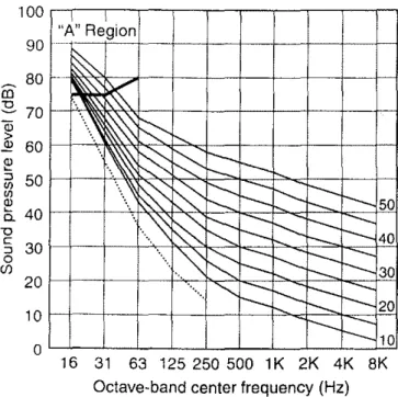
16 31 63 125250500 1K 2K 4K 8K

Octave-band center frequency (Hz)

Fig. J - NCB room noise criteria curves-After ANSI SJ2.2 and Beranek. The dashed line is the approximate threshold of hearing.

IIJ US, Army Construction Engineering Research Lab, PO. Box 9005.

Champaign.JL 61826·9005 US.A., schomer@uiuc.edu

h) NariOlwl Research Council, Institue for Research in COllstmciton.

()t/(/\\'(jOntario KIA OR6, Canada, joh1l.bradley@nrc.ca

1. INTRODUCTION

The recent American National Standard, Criteria for

Evaluating Room Noise,l presents two sets of room noise

criteria curves; one tenned NCB and the other RC. The NCB criterion curves are given in Fig. 1 and Table 1. They appear in the ANSI Standard only as a table of values. Beranek derived these curves from the characteristics of hearing to be consistent with equal-loudness-level contours and to be

OClave-band NCB NCB NCB NCB NCB NCB NCB NCB NCB center 50 45 40 35 30 25 20 15 to frequency (Hz) 16 89 87 85 83 82 81 81 81 81 31 80 77 74 71 68 66 64 62 61 63 68 65 61 58 54 51 48 45 43 125 63 59 55 51 47 43 38 35 3 t 250 58 53 49 44 39 35 30 26 21 500 55 50 45 40 35 30 25 20 t5 1000 52 47 42 37 32 27 22 17 12 2000 48 43 38 33 28 23 18 13 8 4000 45 40 35 30 25 20 15 10 5 8000 42 37 32 27 22 17 12 7 2

TABLE 1 - Numerical values for Ihe NCB curves.

consistent with subjective responses.2_{TheRC criterion curves}

are given in Fig. 2. They are parallel lines with a -S dB per octave slope that goes through the stated RC value in the 1000 Hz octave band. These curves appear in the ANSI Standard only as a table of values. Blazier derived these curves from subjective responses to include the effects of slowly

fluctuating ｬｯｷｾｦｲ･ｱｵ･ｮ｣ｹ noise.3_•4

The two sets of room criterion curves each are based on data and theory, and each is correct for a specific set of situations. These two sets of criterion curves depart most markedly from one another at low frequencies and low sound levels. Also, each set has its problems. The RC curves set criteria levels that are below the threshold of hearing. This is done to protect against modern, poorly designed HVAC systems that generate large turbulent fluctuation at low

frequencies and can include fan surgingwithconcomitant noise

level surging of 10 dB or more. But the RC curves, strictly utilized, would "penalize" a well designed HVAC system such as the type that might be included in a concert hall design. The RC criterion could require 10 dB or more of unnecessary noise quieting at low frequencies. On the other hand. the NCB

ＢｾＬＬ

Relgion ｾＮ｟Ｎ

ｾ

I

-｜｜ｾ

_ｾ

ﾷｲｾ

_{ｾ ｾ ｾ}

r----ｾ

ｾ

t::-

c..:::::

!'-

t--

r--

50

｜｜ｾ

_ｾ

_::::::-

_--:::::

---

t-

--:::::

40

..

..

ｾ

ｾ

r--::

!'-

t-

r--::

..

30

.'.

'"

-=:

_---

f=:-

--:::::

20

r---

_c-.::::

₁₀ 100 90

CO

80 ｾ ₇₀ Qj > ｾ 60

E!

:J ₅₀ VI VI OJ ｾ 40 Cl. -0 c: 30 :J 0 (/) 20 10 0

l'\.

t\.'

ｾ

90 ho ｾ｜

_...

₈₀

_t'...

...

70

t'...

r-...

60

t'...

f'....

50

t'...

,

... 40

t'...

r-.."""-

30

...

:"-.

...

20

t'...1-""

...

₁₀

t'...1-...

0

t'...

....

_...

Frequency (Hz) 16 31 63 125250500 1K 2K 4K 8K

Octave-band center frequency (Hz)

130 120 110 _ 100 (l] ｾ 90 (jj ₈₀ > .'!! ₇₀ [l! 60 :J <n <n ₅₀ [l! Q. ₄₀ -0 c ₃₀ :J 0 (f) 20 10

a

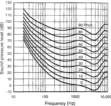
ｾ10 10 100 1000 10,000

Fig. 2 - RC room noise criteria curves-After ANSI SJ2.2 and Blazier,

The dashed line is the approximate threshold of hearing.

curves set criteria levels that are based on Ｂｷ･ｬｬｾ｢･ｨ｡ｶ･､Ｂ

HVAC systems-systems where turbulence generation is

minimized and fan surging does not exist. As such, these

criteria aTC inappropriate,alone, for a standard. They do not

protect the user from a poor system (a turbulence-generating

ｦ｡ｮｾｳｵｲｧｩｮｧ system) that still can legally meet the standard.

There can be no doubt that lawyers could and would use the

NCBcriteria to show that their poor system met the standard.

ｓ｣ｨｯｭ･ｲｾ has suggested the RNC curves and associated

methodology as a means to Tatc rOom noise that bridges the

gap between Beranek and Blazier. For well-designed HVAC

systems,itsets criteria that are very similar to the NCB criteria

of Beranek. However,ifthere are large turbulent fluctuations

at low frequencies and/or fan surging with concomitant noise level surging, then the RNC methodology includes penalties that, in effect, reduce the criteria to those that are similar to the RC criteria of Blazier. The RNC methodology is based on

theories for hearing. It makes extensive use of the

equal-ＱＰｵ､ｮ･ｳｳｾｬ･ｶ･ｬ contours of the ear (Fig. 3). These contours

show that for a constant increase in sound pressure level, the increase in loudness is much greater at low frequencies than at frequencies above about 250 Hz, and that this effect increases

with decreasing frequency. Because of this low-frequency

effect, the RNC methodology incorporates two factors.

First, because of this ｬｯｷｾｦｲ･ｱｵ･ｮ｣ｹ effect, the RNC

contours are spaced more closely together at low frequencies and lower sound pressure levels than at the frequencies above 250 Hz. Second, because of this low-frequency effect, it is inappropriate to use the equivalent level (LEQ) in octave bands as the descriptor. Rather, below the 250 Hz octave band, sound must be combined into critical bandwidths and integrated over short periods that correspond to the integration time of the car. That is, time-series of LEQ levels are developed for the combined 16, 31 and 63 Hz octave bands (the first critical band), for the 125 Hz octave band (the second critical band),

Noise Control Eng. J. 48 (4), 2000 Jul-Aug

Fig. 3 - Equal-loudness-level contours (After ISO 226).

and for each octave band above 125 Hz. Provisionally,

Schomer suggested using the 125 ms integration time of

fast-time weighting to approximate the integration fast-time of the ear.5

To create the time-series ofLEQ levels, the fast-time-weighted level was to be sampled sufficiently fast to follow the

fast-ｴｩｭ･ｾｷ｣ｩｧｨｴ･､ signals. A sample rate of about 100 ms was

suggested. Following generally accepted practice, it was

assumed that the critical bands of the ear were about 100 Hz

wide at frequencies below500Hz. Therefore the three lowest

frequency octave bands (] 6, 31, and 63 Hz) are combined together when forming the time series since together they are about 100 Hz wide.'·' The t25 Hz octave band was used by itself when fonning the time series since it is about 100 Hz wide by itself. All octave bands above 125 Hz were used each alone, since each is greater than 100 Hz wide.

Equation(I)gives the method to sum the levels from any

of the time series. In Eq. t, the parameter d reflects the sound pressure level increase required for a 10 phon increase in loudness at low to moderate sound levels (Fig. 3). For the lowest band (the combined 16,3 I, and 63 Hz octave bands), d was set to 5. For the 125 Hz octave band, d was set to 8, and for all other bands, d was set to 10.

16 31 63 125 250 500 1K 2K 4K 8K Octave-band center frequency (Hz)

CD

90 ｾ 80

Ｍ｟ｾ

70

60

ｾ

50

ｾ

40

Q. 30

1!

20

5

10

(/)

0

In Eg. (1), Ljis the ith value of any time series, N is the

number of elements to that time series,L_mis the mean value

for that time series, and LLL is the calculated result for that

ti me series. Note that for 0 equal 10 10, Eq. (I) reducestothe

equation normally used to calculate LEQ. That is, for the

250 Hz octave band and above, the RNC metric reduces to

octave band LEQ levels.

Bradley has studied the annoyance generated in rooms by sounds that contain various degrees of turbulence and surging at low frequencies. s He reports on an initial experiment 10 evaluate the additional annoyance caused by varying amounts of low-frequency rumble sounds from heating, ventilating, and air conditioning (HVAC) systems. HVAC noises were simulated with various levels of low-frequency sound and varying amounts of amplitude modulation of the

low-frequency components. Nine subjects listened to the test

sounds over headphones and adjusted the level of the test sounds to be equally annoying as a fixed neutral reference sound. The neutral test sound was random noise with a minus 5 dB per octave slope to the spectrum. Bradley used time-series of short-term LEQ levels to evaluate these sounds. The short-tenn LEQ levels were calculated each 0.128 s for each one-third-octave band. Thus, these data can be used to test the RNC methodology. The 0.128 s LEQ levels certainly approximate a series of fast-time-weighted levels, and the energies in the 16, 31, and 63 Hz octave bands can be combined according the RNC methodology. The resulting RNC levels can be compared with the psycho-acoustical evaluations provided by Bradley's subjects. This paper uses the Bradley data to test the RNC methodology.

2. EVALUATION OFTHE BRADLEY DATA A. The Bradley data

The Bradley data consisted of 25 test signals' Five signals consisted of random noise with 5 degrees of rumble, the higher the rumble the higher the LEQ in the lower frequency octave bands. Levels were increased by increasing the gain and the

standard deviation to the noise. These 5 signals had no

amplitude modulation to simulate fan surging. Little could be done with the 16 Hz octave band in this experiment because it used headphones and could not reproduce energy at this low frequency. Primary use was made of the 31 Hz octave band.

Bradley used the highest two rumble signals for the modulation experiment. He designated these as the "low" and "high" rumble signals. Each rumble signal was modulated at two levels, 10 and 17 dB, which he designated as "low"

and "high" modulation. For each level of rumble and

modulation he used 5 modulation frequencies: 0.25, 0.5, I,

2, and 4 Hz. Thus, in the Bradley study there were 20

modulated test signals to go with the 5 un-modulated test signals. Bradley's choice of modulation frequencies centers on the important range, since, according to Blazier, a modulation frequency of I Hz is typical of HVAC problems.' The original two un-modulated rumble spectra used for the modulation experiment and the control signal spectra arc shown in Fig. 4. Further details of the original experiment can be found in Bradley.s

126 Noise Control Eng. J, 48 (4), 2000 Jul-Aug

There were no analogue or digital recordings of these test signals, but digital data records of the LEQ by one-third-octavc band, for every 0.128 s arc available for all 20 modulated test signals and for the highest two un-modulated, rumble test signals (Fig. 4). Each digital record consists of 559 samples, each 0.128 s in duration.

Each of the 9 subjects compared separately each of the 24

test signalstothe neutral, reference spectrum. To do this, the

subject would adjust an attenuator that conu-olled the test signal

until that subject judged the test signaltobe equal in annoyance

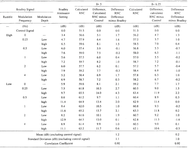
to the reference spectrum. Table 2 lists the average attenuator setting for the 22 test signals for which there are digital records. Note that Bradley found that the reference spectrum when compared to itself yielded an attenuator setting of just 0.2 dB showing good internal conslstency for this experiment.

B. Testing the RNC methodology

In concept, testing of the RNC methodology using the Bradley data is straight forward. One would evaluate the RNC level for each of the 25 test signals, subtract the RNC level for the reference spectrum from each of the other 24 test signal RNC levels, and compare these 24 differences with the corresponding 24 mean attenuator settings. Unfortunately there are two difficulties with accomplishing this task. First, no digital record is available for the reference spectrum by 0.128 s time slices although the LEQ by one-third-octave band for the entire 71.5 s is available. However, the reference signal is described as not rumbly and it clearly is un-modulated. Therefore, for this analysis we must assume that the reference signal is non-surging and with a small enough standard deviation such that the octave band LEQs can be used to detennine the RNC level without any penalties.

Second, the Bradley data are for relatively high sound levels,

and they are beyond the levels given in Schomer.5 _{In fact, the}

LEQs in the 31-Hz octave band are well into the rattle region, which is designated the "A"Region by both Beranek and Blazier and also by the RNC method. There are at least two methods to extend the RNC curves to higher levels and these are portrayed in Figs. 5(a) and 5(b). In Fig. 5(a), the RNC curves have been extended in an analytic fashion to higher levels. At

ｾ • Control

IIILower Rumble

LJHiqher Rumble

til

,

fl"g. 4 - Original Bradley spectrajor the higher rumble, the lower Tumble and the control conditions. No modulation is present for these spectra.

TABLE 2 "- Comparison between Bradley a\tenuator setting and the corresponding differences using RNC calculations - - ._-Rumble Bradley Signal Modulation Frequency 00 5 8= 6,25 ._._--_..

-Bradley Calculated Difference, Difference Calculated Difference, Difference

Allenuator RNC Calculated RNC RNC calculated RNC

Modulation Selting RNC minus Difference RNC minus Difference

Depth Control minus Bradley Contra] minus Bradley

Mean (dB) (excluding control signal) Standard Deviation(dB)(excluding control signal)

Correlation Coefficient (Hz) Control Signal J-ligh 0 0.25 0.5 2 4 Low 0 0.25 0.5 2 4 (dB) (dB) (dB) 0.0 51.5 0.0 3.4 56.6 5.1 Low 4.7 57,9 6.4 high 6.5 596 8.1 Low 6.0 57.4 5.9 high 7.6 590 7.5 Low 5.6 57.5 6.0 high 7.2 59,7 8.2 Low 6.0 57.7 6.2 high 7.9 59.2 7.7 Low 5.2 58.4 6.9 high 6.9 58.7 7.2 5.9 59.6 8.1 Low 7.5 61.8 10.3 high 9.7 65.5 14.0 Low 8.6 61.2 9.7 high 11.4 649 13.4 Low 9.4 62.0 10.5 high 11.6 652 13.7 Lnw 8.2 61.6 10.1 high 12.9 64,5 13.0 Low 8.9 6J4 9.9 high J1.J 632 II.7 (dB) (dB) (dB) (dB) 0,0 51.5 0.0 0.0 I.7 56.2 47 1.3 1.6 57,2 5,7 1.0 1.5 585 7.0 0.4 -0.1 56.8 53 -0.7 -02 58.0 6.5 -1.1 0.4 570 55 -0.2 1.0 58.7 7.2 -0.1 0.1 57.2 5.7 -0.4 -0.3 58.4 6.9 -1.0 I.7 57.8 6.3 1.0 0.3 58.2 6.7 -0.2 2.1 59.2 7.7 l.7 2.7 60.5 9.0 1.5 4.3 63.4 ] 1.9 2.2 1.1 60.4 89 0.3 2.0 629 JI .4 0.0 1.0 60.8 9.3 -0.2 2.1 63.3 11.8 0.2 1.9 60.7 9.2 1.0 0.1 628 ) 1.3 -1.6 1.0 60.5 9,0 0.1 0.6 621 10.6 -0.5 1.2 0.2 1.1 1.0 0.92 0.92

and above the 250 Hz octave band, the curves are 5 dB apart. In the 31 Hz octave band, the curves increase by 2.5 dB in sound pressure level for each 5 unit increase in RNC. Obviously, this extension leads to curves such that the slope at low frequencies (below the 250 Hz octave band) is less than the slope above the 250 Hz octave band. Several relations and procedures suggest that this extension is not logical. First. the loudness functions (Fig. 3) never exhibit this type of slope relationship. Also, the loudness function and the Beranek curves (Fig. 1) increase in their spacing with increasing sound pressure level. The Blazier curves (Fig. 2) maintain a constant spacing, but this is a constant 5 dB at all frequencies.

Figure 5(b) shows the RNC curves extended to higher levels by adding curves that are everywhere parallel to the RNC 50 curve. This is, perhaps. the more logical extension sinee, firstly, it follows the Blazier lead of 5 dB parallel spacing. Second, like the equal-loudness-level contours and like the NCB curves, it increases the spacing at low frequencies and higher sound pressure levels. Third, it does not exhibit the strange reverse in slope that is evident in Fig. 5(a) but not present in equal-loudness-level contours. For

these reasons, this paper extends the RNC curvestoRNC 65

as shown in Fig. 5(b).

NoiseControl Eng. J, 48 (4), 2000 Jul-Aug

The functions represented by the eurves in Fig. 5(b) are easily represented analytically for use in a spreadsheet and these functions are given in the Appendix. These are the functions that have been used to evaluate the Bradley data. In this analysis, it is assumed that rattles were not an issue because the subjects listened to the sounds through headphones, although normally, levels this high at low frequencies would have a high probability of creating rattles in building elements.

c.

Results

Table 2 lists the calculated RNC levels minus the reference signal RNC for the 22 Bradley test signals that were available as digital records in the form of 0.128 s time series. As stated earlier, this table also contains the attenuator settings found

for these test signals. In accordance with the RNC

methodology, energies in the 16, 31, and 63 Hz octave bands were combined together after weighting each for the loudness characteristic of the ear. To do this, 14 dB were subtracted from the 16 Hz octave band levels and 14 dB were added to the 63 Hz octave band levels. There were no changes to the 31 Hz octave band levels.

3. DISCUSSION

15 31 63 125250500 lK 2K 4K 8K

Octave-band center frequency (Hz)

Fig.5 - (a)The dashed lines show the extended RNC curves using analytic functions and the solid lines show the original RNC curves. (b) The dashed lines show the extendedRNe

curves using conslant 5-dB differences and the solid lines show the original RNC curves.

Examination of the data in Table 2 shows that there is good correlation between the attenuator setting and the calculated RNC differences. This correlation coefficient is

0.92. More importantly, the standard deviation to the

djfferences is only 1.1 dB. However, there is a systematic

difference of 1.2 dB. Ifthe RNC provided a perfect fit to the

Bradley data, the correlation coefficient would be I, the standard deviation would be 0 dB, and the systematic difference would be 0 dB. Part of the systematic difference

may be due to a correction that should have been applied to

the control signal. But we are unable to calculate any

4. CONCLUSIONS AND RECOMMENDATIONS Based on the Bradley data, the RNC procedure is working well. The efficacy of Eq. I for integrating the low frequency data is clearly demonstrated. Basing the value of 8 in Eq. I on the equal-loudness-level contours also clearly is

correctiontothe control signal because we no longer possess

its time waveform. Any turbulence to the control signal will increase its RNC value and, thus, decrease this systematic offset of 1.2 dB.

Some of the standard deviation of I. I dB and the offset of

J2 dB may result from subject bias and subject variation given

that there were only 9 subjects. Most importantly, some of this variation may be due to the assumptions inherent in the RNC procedure. First, it was assumed that d equal to 5 dB

was applicableto the 3] Hz band since, at low sound levels,

the equal-loudness-level contours (Fig. 3) are spaced 5 dB apart for a change of 10 phon. In this experiment the 31 Hz octave band levels are between 80 and 90 dB. At these higher sound levels, the equal-loudness-level contours are spaced more like 6 dB apart for a change of 10 phon. Therefore, all the data have been reanalyzed with various values for d in the 31 Hz band. Repeated calculations in 0.25 increments have

shown that

8

equal to 6.25 yields the best fit to the Bradley

data. These results are listed in column 6 of Table 2. With

this value of&, the standard deviation to the differences drops

to 0.98 dB, the correlation coefficient remains at 0.92, and the offset drops to just 0.2 dB. As noted above, this trivial

0.2-dB offset is partly due tu any minor turbulence to the

control signal that has not been accounted for. Also, the

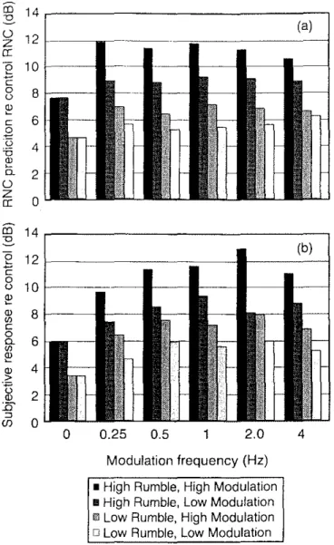
subjects could only replicate their responses to 0.2 dB. Figurc 6(a) shows the Bradley attenuator settings as a function of rumble and modulation, and Fig. 6(b) shows the differences in RNC between the test signals and the control signal for these same conditions. The general similarities between these two figures can be seen. One difference is at low modulation frequencies where the RNC predicts higher differences than were measured by Bradley. No explanation can be offered for this difference. However, one important similarity is at the 4 Hz modulation frequency. The PNC predicted differences are more or less constant from 0.15 to 2 Hz and then reduce at 4 Hz. The Bradley subjective response differences peak at 2 Hz and then reduce at 4 Hz. This downward trend at 4 Hz is consistent with the use of 125 ms as the integration time, the assumed time constant of the ear.

Ifwe had assumed that the time constant was shorter than

125 ms, say 65 ms, then the PNC-predieted differences would not reduce at 4 Hz. If we had assumed a larger value for the time constant of the ear, say 250 ms, then the PNC predicted differences would start to reduce at 2 Hz and there would be a much larger reduction at 4 Hz than is shown in Figure 6(b). In either of these cases, the PNC predicted differences would correspond less well with the differences measured by Bradley. But the RNC calculated difference seems to fit the Bradley data well at 4 Hz. This implies that the selected time constant of 125 ms (fast time weighting) is about optimum.

I

(a) "A"

ｾ･ｧｩｾｮ

---::,,::::'

..., - - " Ｎ｟ｾＮＭＢ

f--:J

ｾ

'...

:

...

:

...

"

... ...

I

ｾｾｾ

...

... ...

... '"

ｾ

_ｾｾ

_t::::

...

... ...

r---

...

'.

"

.

...,

1--

....

'\

_ｾ

ｾ

ｾ r---

'---

_t'--

...

50

----"\

_ｾ

_r-::::

_'---'---

_K:--

::::

50

"\:

_{ｾ r--::::}

r---

t---

_::::::--

40

""

e---:::::

""

t'-

ｾ

30 RN( =10

ｾ

r---

20 '"

_...

(b)

...

'.

....

'.

_...

.

...

_{... "A" Region} '.

...

.

...

ｾ

. /

". "

.

'. ".

....

t:----."-

....

'" '.

...

ｾ '. ".

ｾ ｾｾ

ｾ

".

'. '"

...

....

"

.

...

_..

.

...

_...

ｾｾ

ｾ ｾ

----:

_...'"

..

...

.

...

".

..

_""" ".

_...

'\

_ｾ

_f0:

_ｾ

_---:::

""

t:--

r-...

... 50

"\

_ｾ

_:-=::

_---=:::

""

ｾ

K

50

'"t

"\

_:----::::

""

""

:::::---

;::::-

40

-+

_'"

_r--::::

_r---

_t:--

_ｾ

30

""

r---

20 RN =10 100 90 80

EO

:s

70 Q) >

..'"

50 ｾ OJ ₅₀ U) U) ｾ ₄₀ 0. "D C 30 OJ 0. (J) 20 10 0 10

o

20 100 90 80 OJ

:s

70

ｾ

..'" 50 ｾ ｾ 50 U) ｾ 0. 40 "D

§

30 0. (J)

Modulation frequency (Hz)

Fig. 6 - (a)RNC values re the control of51.5dB. (b) "Atrenuator

" offsets found by Bradley.

• High Rumble, High Modulation • High Rumble, Low Modulation o Low Rumble, High Modulation o Low Rumble, Low Modulation

TABLE A I - Coefficients to theequationsforcalculating RNC

OC1:-lVeBand SoundLevelRange K1 K2

(J 17) (dB) ---_.., ---_._---16 £81 64.3333 3 >81 31 1 ] I [ 76 51 2 >76 26 1 63 £71 37.6667 15 >71 21 I 125 £66 24.3333 1.2 >66 16 1 250 ALL 11 1 500 ALL 6 1 1000 ALL 2 1 2000 ALL -2 1 4000 ALL -6 1 SOO(J ALL -10 1 5. APPENDIX:

Equations for calculating RNC

The RNC in the ith octave band between 16 Hz and 8000 Hz is calculated by equations of the form:

RNC,ｾ (L, - KI)

*

K2,

Where L, is level in the ith octave band. In bands at and

above 250 Hz, L; is just the octave-band equivalent sound

pressure level. In bands below 250 Hz, the general RNC

procedures arc used. If the sound is rumbly or modulated, then Equation 1 is used to calculate levels in for use with the 31-Hz and 125-Hz equations. Table A 1 gives the coefficients for use in calculating the RNC in any octave bands. For octave bands below 250 Hz, the equations are different for RNC values above and below RNC SO. The RNC procedure is a tangent method, so the reported RNC is the maximum of the RNCs calculated for the various octave bands

(a) (b) 2.0 4

co

₁₄ :E-O ₁₂

z

a:

e

10

c

0 ₈ '-'

i"

c

6

.8

u

₄ is Q) Q ₂ 0

z

0

a:

co

14

:E-e

12

c

0

10

'-'

i"

Q) ₈

"'

c 0

6

"-"'

i"

Q) 4 > "f) 2 Q) 15' ::> (f) ₀ 0 0.25 0.5

1

6. REFERENCES

demonstrated. Finally, the use of a 125 ms time constant to approximate the time constant of the ear has been demonstrated to be a successful approximation to the time

constant of the hearing system. These three arc the main

features that are inherent in the RNC calculation, and all have been validated by the Bradley data.

Use of the RNC procedure as described in Schomer' with the curves as given in the Appendix to this paper is recommended.

Although, at high levels, 0 equal to about 6 provides for slightly better results, a 0 equal to 5 in the 31 Hz band and a

o

equal to 8 in the 125 Hz band is recommended at all sound

Icvels. The added complexity of changing 0 with sound level is not worth the increased accuracy by about I dB at high sound levels. Simply put, when the sound level is over 80 dB

in the 31ｾｈｺ octave band, onc can afford to over-predict the

RNC by I unit.

American National Standnrd Criten'afor Evaluating Room Noise, American

National Standards Institute, ANSI S12.2-1995 (Acoustical Society of America, New York, 1995).

Leo Beranek, "Applications of NCB and RC noise criterion curves for specification and evaluation of noise in buildings," Noise Control Eng. J.

45(5).209-216 (1997).

Warren Blazier, "Revised noise criteria for application in the acoustical design and rating of HVAC systems," Noise Control Eng.J.16(2),64-73 (198]). Warren Blazier, "RC Mark JI; a refined procedure for rating the noise of heatIng, ventilating and air-conditioning (HVAC) systems in buildings," Noise Control Eng. 1. 45(6), 243-250 (l997).

Paul Schomer, "Proposed revisions to room noise criteria calculations," Noise Control Eng.J.48(3), 85-96 (2000).

Arnold M. Small and Robert S. Gales, Handbook of Acoustical

Measurements and Noise Control, 3rd Edition, Chapter 17, Hearing Characteristics, Cyril M. Harris, Ed. (McGraw Hill, Inc., I991).

E. Zwicker, G. Flottorp, and S. S, Stevens, "Critical band width in loudness summation," 1. Acoust. Soc. Am. 29(5),548-557 (1957).

John Bradley, "Annoyance caused by constant-amplitude and amplitude-modulated sounds containing rumble," Noise Control Eng.J.42(6),

203-208 (1994).

9 Warren Blazier, Personnel communications (2000).