HAL Id: halshs-01734745
https://halshs.archives-ouvertes.fr/halshs-01734745v2
Preprint submitted on 12 Sep 2019HAL is a multi-disciplinary open access
archive for the deposit and dissemination of sci-entific research documents, whether they are pub-lished or not. The documents may come from teaching and research institutions in France or
L’archive ouverte pluridisciplinaire HAL, est destinée au dépôt et à la diffusion de documents scientifiques de niveau recherche, publiés ou non, émanant des établissements d’enseignement et de recherche français ou étrangers, des laboratoires
Contribution to a Public Good under Subjective
Uncertainty
Anwesha Banerjee, Nicolas Gravel
To cite this version:
Anwesha Banerjee, Nicolas Gravel. Contribution to a Public Good under Subjective Uncertainty. 2019. �halshs-01734745v2�
Working Papers / Documents de travail
Contribution to a Public Good under Subjective Uncertainty
Anwesha Banerjee
Nicolas Gravel
Contribution to a Public Good under Subjective
Uncertainty
∗
Anwesha Banerjee
†and Nicolas Gravel
‡August 29th 2019
Abstract
This paper examines how voluntary contributions to a public good are affected by the contributors’ heterogeneity in beliefs about the uncertain impact of their contributions. It assumes that contributors have Savagian preferences that are represented by a two-state-dependent expected util-ity function and different beliefs about the benefit that will result from the sum of their contributions. We establish general comparative statics results regarding the effect of specific changes in the distribution of be-liefs on the (unique) Nash equilibrium provision of the public good, under certain conditions imposed on the preferences. We specifically show that the equilibrium public good provision is increasing with respect to both first and second order stochastic dominance changes in the distribution of beliefs. Hence, increasing the contributors’ optimism about the uncertain benefit of their contributions increases aggregate public good provision provision, as does any homogenization of these beliefs around their mean. Keywords: Voluntary provision, public good, uncertainty, beliefs, optimism, consensus.
JEL classification codes: C72, H41
"The debate’s over. The people who dispute the international consensus on global warming are in the same category now with the people who think the moon landing was staged on a movie lot in Arizona." (Al Gore)
"Whether global warming or climate change. The fact is: we didn’t cause it. We cannot change it." (Donald J. Trump)
∗With the usual disclaiming qualification, we are indebted to Yann Bramoullé, two
anony-mous referees and an associate editor of this journal for their extremely insightful comments and to Sebastian Bervoets and Arunava Sen for helpful discussions. The second author also gratefully acknowledges the financial support of the French Agence Nationale de la Recherche (ANR) through the grant "The Measurement of Ordinal and Multidimensional Inequalities" (ANR-16-CE41-0005)".
†Aix-Marseille Univ., CNRS, EHESS, Centrale Marseille, AMSE, 5, Boul. Maurice
Bour-det, 13001 Marseille France Cedex, [email protected].
‡Centre de Sciences Humaines, Aix-Marseille Univ., CNRS, EHESS, Centrale Marseille,
1
Introduction
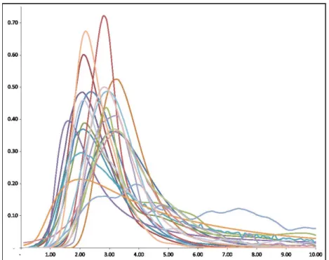
There are many situations where agents are uncertain about the benefit they get from contributing to a public good. The fight against global warming through carbon emission reductions is an example of such a situation. As shown on Figure 1, borrowed from Millner, Dietz, and Heal (2013), there is considerable scientific uncertainty about the impact of carbon accumulation on the Earth’s temperature at the 2050 horizon. Moreover, as is also apparent in the picture, there is significant heterogeneity amongst scientists themselves regarding the probability that they assign to increases in the Earth’s temperature associated with specific scenarios of carbon accumulation (such as the "business as usual" one on Figure 1). This heterogeneity in beliefs about the impact of carbon emis-sions is also reflected in the variety of (less scientific) opinions on this matter found in public debate, and illustrated by the polarized views of the two leading American political figures quoted above. There is little doubt that a person’s belief about the impact of carbon emissions on global warming will affect this person’s propensity to make costly efforts to prevent climate change (see for ex-ample Roser-Renouf, Maibach, Leiserowitz, and Zhao (2014)). After all, had he been the US president, Al Gore would have certainly not taken the same decision vis-à-vis the Paris agreement on global climate change as that taken by Donald J. Trump. Other examples of contributions to a public good under subjective uncertainty include contributions to charities or philanthropic institutions by agents who are uncertain about their reliability or effectiveness, individuals’ de-cisions to vaccinate (see e.g. Brewer, Chapman, Gibbons, Gerrard, and McCaul (2007)) or, in developing countries, to defecate in the open rather than in toi-lets (see e.g. Clasen, Boisson, Routray, Torondel, Bell, Cumming, and Ensink (2014)).
The purpose of this paper is to examine, in a somewhat general model of voluntary provision of a public good, the impact of heterogeneity in beliefs on the agents’ aggregate contribution. We specifically ask two broad questions:
1) Does the increase in some (or all) contributors’ optimism about their contributions to a public good increase the total amount of these contributions? That is, would the US make more effort to reduce carbon emissions if some, or all, of the US citizens who currently share Donald Trump’s beliefs about human-made global warming switch to Al Gore’s view on this matter?
2) Does an increase in the consensus on the impact of individual contribu-tions to a public good increase the overall level of provision? That is, would Donald Trump and Al Gore together contribute more to the fight against global warming if they could bring their different beliefs closer to each other?
These questions are asked in a setting analogous to the classical Bergstrom, Blume, and Varian (1986) setup, but with the important difference that the subjective benefit of any combination of individual decisions is uncertain, and that individuals differ in their perception of this uncertainty. The uncertainty is regarding two possible states of the world: an optimistic one, in which the individual perceives the impact of contributors on public good provision in a favorable way and a pessimistic one in which the individual is more skeptical about the benefit of contributing. Individuals differ in the probability that they attach to these two states. Optimistic individuals, like Al Gore, would attach a probability close to 1 to the first state. On the other hand, pessimistic (or skeptical) individuals like Donald J. Trump would attach almost zero
proba-Figure 1: Estimated distributions of increase in the Earth temperature (in cel-sius) by 2050 under a business as usual scenario (Source: Millner, Dietz, and Heal (2013)).
bility to the same optimistic state. But more intermediate attitudes between these two extremes are certainly possible. We assume that an individual would evaluate his/her contributive decision by the expectation - taken over his/her beliefs - of the same state-dependent utility. Just like in standard models of voluntary public good provision à la Bergstrom, Blume, and Varian (1986), state-dependent utility is taken to be a function of two variables: individual effort (given aggregate public good provision) and public good provision (given individual effort). In either the optimistic or the pessimistic state, the state-dependent utility function is decreasing with effort, increasing with the public good, and concave with respect to the two variables. We also assume that the marginal disutility of effort is not strictly decreasing with respect to the total amount of public good. In such a setting whatever the distribution of beliefs among contributors, it is not hard to prove that there will be a unique Nash equilibrium level of contributions.
This paper identifies the impact of specific changes in the distribution of beliefs on the (unique Nash) equilibrium aggregate level of contributions. We first establish easily that every individual’s equilibrium level of contribution is increasing with respect to his/her own belief. This implies that individuals’ contributions will be ordered by their beliefs at a Nash equilibrium. We then show that an increase in optimism in the population in the sense of first-order dominance (see e.g. Hadar and Russell (1974)) leads to an increase in the aggregate contribution to the public good. The most important result of the
paper concerns the impact of an increase in the consensus about the probability of being in the optimistic state on the overall level of contribution. Assessing this impact requires a definition of what it means for a distribution of beliefs to be “more consensual” than another. Borrowing here again from the stochastic dominance literature, and exploiting the two-state feature of our framework, we define a distribution of beliefs to be more consensual than another when the dominating distribution has the same average belief as the dominated one and has been obtained from the latter by a finite sequence of Pigou-Dalton transfers of probabilities attached by individuals to the optimistic state. We observe that the generalization of this plausible notion of homogenization - or increase in consensus - to more than two states is not immediate. Under some additional conditions on the utility function, we show that the homogenization of beliefs in this sense always leads to an increase in the equilibrium aggregate contributions when the homogeneization takes place among strict contributors.
Our paper contributes to two strands of literature. First, we add to the lit-erature on public goods under uncertainty, by introducing agents’ heterogeneity in the perception of this uncertainty. Second, we contribute to the literature on distributional comparative statics for aggregative games and games with strate-gic substitutes.
The literature on voluntary provision of public goods, initiated largely by Bergstrom, Blume, and Varian (1986) (see also Andreoni (1988)) is rather vast. Yet there is relatively little research that examines the impact of uncertainty on public good provision. Some, like Austen-Smith (1980) or Sandler, Sterbenz, and Posnett (1987), have considered uncertainty regarding the actions of others.1 Our paper does not have much to say on this matter. Gradstein, Nitzan, and Slutsky (1993) is one of the first papers that we know that has examined the im-pact of uncertainty on the benefit from a public good. It has done so by examin-ing the specific impact of price uncertainty on public good provision in a settexamin-ing à la Bergstrom, Blume, and Varian (1986). There is also a large literature, nicely summarized by Gradstein, Nitzan, and Slutsky (1992), that addresses the issue of uncertainty in general non-cooperative games without specific concerns for games of voluntary provision of a public good. There is also a sizable literature devoted to the related issue of bargaining and negotiation regarding public good provision under uncertainty. For example, Kolstad (2007) studies self-enforcing international agreements under systematic or common uncertainty, while Bra-moullé and Boucher (2010) extend the treaty formation model of Barrett (1994) to the case of uncertainty for both a public good and a public "bad". However, these papers suppose risk neutrality on the part of the negotiators who are also often assumed to face the same uncertainty. Schumacher (2015) builds and em-pirically tests a model in which beliefs of individuals influence their willingness to contribute to expenditures towards a cause, such as preventing climate change. However Schumacher (2015) assumes that utility is linear in income, and that there are only two groups of individuals (optimists and pessimists). Moreover, in Schumacher (2015), individuals’ contributions only determine the probabil-ity of occurrence of a common shock which affects the percentage of their final income. Hence, the uncertainty analyzed in Schumacher (2015) is very different from that considered in this paper. Bramoullé and Treich (2009) examine the
1Classical papers on conjectural variations and "non-Nash conjectures" about the reaction
of others such as Cornes and Sandler (1984), Cornes and Sandler (1985) and Sugden (1985) or Itaya and Shimomura (2001) also belong to this stream of literature.
impact of uncertainty regarding the benefit of collective action with risk-averse agents. They show that the introduction of uncertainty can, under some condi-tions, lower the amount of a public bad or increase the amount of a public good. However Bramoullé and Treich (2009) assume that all contributors face the same uncertainty and, therefore, do not examine the impact on public good provision of the contributors’ heterogeneity in their perceptions of uncertainty. There is also a significant literature that has examined the possibility that contributors could be uncertain about others’ valuations of the public good, either in the set-ting of Bergstrom, Blume, and Varian (1986) where the public good provided is the sum of the individual contributions, or in the "Weakest-Link" setting (see for instance Barbieri and Malueg (2019)) where the provided public good is the smallest of all individuals contributions. Bac (1996) has considered an infinitely repeated game between two contributors who have beliefs about the preferences of the other. Bag and Roy (2008) and Bag and Roy (2011) have analyzed se-quential and simultaneous games of voluntary contribution to a public good in the case where each contributor knows his/her own preference type but not the type of the others. Their analysis assumes that all contributors have quasi-linear preferences, and that the types are drawn from the same probability distribu-tion. Hence, they do not address the issue of the possible heterogeneity of the contributors’ beliefs. A paper that does examine this heterogeneity in beliefs is Maldonado and Rodrigues-Neto (2016). It considers the case where contributors have quasi-linear and logarithmic preferences and differ by both their valuation of the public good (measured by a coefficient that multiplies the logarithmic part of their utility) and their belief about the distribution of valuations in the population. The analysis compares the Nash equilibrium that arises when there is incomplete information about the other types and a situation where such in-complete information is not present. However, it does not address the issue of what happens - given incomplete information - when the potential contributors’ beliefs change. All in all, this literature is concerned with the uncertainty about the characteristics of fellow contributors. The framework of analysis is therefore one of incomplete information. This literature does not examine, in a situation of complete information such as that considered here, the issue of uncertainty regarding the benefit of individual contributions to the public good. To the best of our knowledge, the only paper that deals with heterogeneity of beliefs on the benefit of public good provision is Sakamoto (2014). Yet this paper analyzes the impact of the different beliefs that contributors assign to a collection of different probability distributions over the possible benefits of public good pro-vision. The considered framework is therefore that of objective ambiguity (see e.g. Ahn (2008) or Gravel, Marchant, and Sen (2018)). By contrast, the current paper does not suppose any ambiguity. It rather examines to what extent the diversity of non-ambiguous beliefs about the impact of individual contributions affects the overall level of public good provision.
As for the theory of distributional comparative statics in aggregative games, the literature that grows in the tradition of Topkis (1978) has established quite general results for games where the players’ actions are strategic complements. A good summary of these results is provided by Milgrom and Shannon (1994). However, general results for games in which the players’ strategies are strategic substitutes - like games of voluntary contributions to a public good such as Bergstrom, Blume, and Varian (1986) - are much more sparse. Corchòn (1994) provides powerful comparative statics results for the case where players have
strongly concave payoff functions. These results by Corchòn (1994) have been generalized significantly by Acemoglu and Jensen (2013). However, these papers only consider the impact of monotonic changes in the exogenous parameters of the models (for instance, individuals’ beliefs) on the equilibrium. They do not explore the impact of non-monotonic changes in the distribution of those parameters. Jensen (2017) provides comparative statics of certain specific types of changes in the distribution of individual parameters in the context of Bayesian games.
The rest of the paper is organized as follows. The next section introduces our model of voluntary contributions to a public good with uncertainty and heterogeneous beliefs. The main comparative statics results are provided and discussed in Section 3 and Section 4 concludes.
2
The Model
We consider a community made of a set N = {1, 2, ..., n} of n agents (with n ≥ 2)). Any agent i ∈ N must choose a level ei∈ [0, e] of effort (say in carbon emission reductions), where e is some strictly positive number, interpreted to be the maximal amount of effort that any agent can make. Two natural interpreta-tions of effort in our model come to mind. One could view it as reflecting the time spent on the collective activity (for instance lobbying). In this case, the effort endowment e would measure some maximal time availability that an agent can have. Another interpretation, more in line with the classical Bergstrom, Blume, and Varian (1986) model, would interpret effort in monetary terms. If this in-terpretation is favoured, then e would be interpreted as the agent’s contributive ability, which would therefore be taken to be same for all agents. Any given profile (e1, ..., en) ∈ [0, e]n of efforts made by the agents generates an aggregate public good G = ni=1eithat they all value. Each agent is, however, uncertain about his/her subjective evaluation of any combination (e, G) ∈ [0, e]× [0, ne] of his/her effort and the aggregate public good produced by the sum of agents’ efforts. The uncertainty concerns specifically two possible states of "optimism" (Al Gore) or "pessimism" (Donald J. Trump) about the effect of agents’ efforts on public good provision. If the optimistic state o materializes, then a given com-bination (e, G) of effort and aggregate public good yields a utility of Uo(e, G). On the other hand, if the pessimistic state p happens, then the utility provided by this very same combination is Up(e, G). Agents differ in their beliefs about the likelihood of the optimistic state. Agent i believes the true state to be opti-mistic with probability πi∈ [0, 1]. Such an agent will evaluate the combination (e, G) ∈ [0, e]× [0, ne] of effort and aggregate public good by the expected state dependent utility EU (πi; e, G) defined by:
EU(πi; e, G) = πiUo(e, G) + (1 − πi)Up(e, G) (1) We assume throughout that the functions Uo and Up are at least thrice differentiable2 with respect to their two arguments and are both decreasing with respect to effort, increasing with respect to the aggregate public good and strictly concave.3 We also assume that Up(e, G) ≤ Uo(e, G) for any combination
2The (partial) derivative of a function g with respect to its jth argument is denoted by g j. 3That is, the function Uj (for j = o, p) satisfies Uj(λe + (1 − λ)e′, λG+ (1 − λ)G′) >
of effort and aggregate public good (e, G) ∈ [0, e]× [0, ne] (given effort and the level of the public good, optimism is weakly preferable to pessimism). A degenerate case of this model happens of course when Uoand Up are the same functions and when, as a result, there is no uncertainty about the benefit of contributing and no heterogeneity among individuals. Functions Us(for s = o, p) are also assumed to satisfy Us
eG(e, G) = UGes (e, G) ≤ 0 for any (e, G) ∈ [0, e]× [0, ne]. This assumption rules out the possibility for the (subjective) marginal cost of effort to be strictly decreasing with respect to the public good. The weak formulation of the assumption makes it compatible with the possibility that either (or both) the functions Uoand Upbe additively separable with respect to their two arguments. We finally assume that Us
e(0, 0)+UGs(0, 0) > 0 > Ues(e, G)+ Us
G(e, G) for any G ∈ [0, ne] and s = o, p. The first part of this assumption says that an agent would always want to contribute at least a little bit when nobody is contributing. The second inequality of this assumption says that an agent would never choose to contribute all his/her effort endowment. This assumption rules out from the start Nash equilibria where nobody contributes and, at the other extreme, Nash equilibria where some agents contribute all their effort endowment. However this assumption allows for Nash equilibria where some, but not all, agents do not contribute. We denote by U the set of all pairs of functions Uoand Up that satisfy these properties.
This framework is general enough to describe many situations of contribu-tion to a public good under uncertainty examined in the literature. A special case of the above model would be one where, for s = o, p, one has Us(e, G) = −C(e) + Φs(G) for some state independent increasing and convex cost function C and some increasing and concave state dependent function Φs. In the context of preventing global warming, such a specification, used notably by Bramoullé and Treich (2009), is somewhat natural. The cost - say in dollars - of preventing global warming by devoting costly immediate effort in carbon emission reduc-tions could plausibly be independent from the subjective appraisal of the impact of aggregate carbon emissions on global warming. The state dependent function Φs would measure, on the other hand, the monetary benefit of global warming reduction in state s of the impact of aggregate human efforts - as measured by G. This monetary benefit would naturally be assumed to be an increasing and concave function of the total effort in carbon emission reductions. As a matter of fact many contributions to the literature on the negotiation process leading to international agreements on the prevention of global warming have considered even more restrictive versions of this model. For example Ulph (2004) considers countries involved in such a negotiation process with a linear utility function of the form −be + cG for some strictly positive real numbers b and c. Kolstad (2005) considers a quadratic version of the same model.
Any distribution of beliefs π = (π1, ..., πn) ∈ [0, 1]n in the population gen-erates the game in strategic (or normal) form G(π) in which N is the set of players, [0, e] is the strategy set of any such player, and EU (πi; ei, ei+
j=i ej) is the payoff received by player i at the strategy profile (e1, ..., en) ∈ [0, e]n when he/she holds belief πi. Observe that πi is the only determinant of player i’s payoff in such a game. It is easy to see that the game G(π) is what has been called by Corchòn (1994) an aggregative game (see also Dubey, Mas-Colell, and
λUj(e, G) + (1 − λ)Uj(e′, G′) for every λ ∈]0, 1[ and every distinct combinations (e, G) and
Shubik (1980) and Shubik (1984)). A (pure strategy) Nash equilibrium for the game G(π) is an effort profile (e∗
1, ..., e∗n) ∈ [0, e]nsuch that, for every individual i ∈ N and effort level ei∈ [0, e] for this agent, one has:
EU(πi; e∗i, e∗i + j=i
e∗j) ≥ EU (πi; ei, ei+ j=i
e∗j) (2) We start by establishing, in Proposition 1 below, the existence and unique-ness of a Nash equilibrium in pure strategies of the game G(π) for any distrib-ution of beliefs π = (π1, ..., πn) ∈ [0, 1]n. This result is obviously an important preliminary step for identifying the effect of specific changes in the distribution of beliefs on the Nash equilibrium of the game. Such an endeavour can obvi-ously not be achieved if Nash equilibria do not exist for some specification of the beliefs. Moreover, if there are many different Nash equilibria that can result from a particular distribution of beliefs, it is difficult to predict which of them would be achieved if the distribution of beliefs changes.
A preliminary step for establishing this result is the following technical lemma, that establishes some monotonicity properties of the function T : [0, 1]× [0, e] × [0, ne] → R defined, for any (π, e, G) ∈ [0, 1] × [0, e] × [0, ne], by:
T (π, e, G) := π[Uo
e(e, G) + UGo(e, G)] + (1 − π)[Uep(e, G) + U p
G(e, G)] (3) The function T , also analyzed in Corchòn (1994), is nothing but the derivative of the expected state-dependent utility function of Expression (1) with respect to the agent’s effort given the efforts by others. This derivative, that is zero for any agent who contributes a positive amount at a Nash equilibrium, plays for this reason a key role in the characterization of such Nash equilibria. The lemma - proved in the Appendix like all formal results of the paper - is the following. Lemma 1 Let π = (π1, ..., πn) ∈ [0, 1]n be a distribution of beliefs and let G(π) be the associated game in strategic form. Then, if any player i’s payoff of this game writes πiUo(ei, ei+
j=i
ej)+(1−πi)Up(ei, ei+ j=i
ej) for a pair of functions Uo and Up in the set U, the function T defined by (3) is strictly decreasing with respect to both e and G.
Equipped with this lemma, we establish in the following proposition the existence and uniqueness of a Nash equilibrium for the game G(π) for any distribution (π1, ..., πn) of beliefs.
Proposition 1 Let π = (π1, ..., πn) ∈ [0, 1]n be a distribution of beliefs and let G(π) be the associated game in strategic form. Then, if any player i’s payoff of this game writes πiUo(ei, ei+
j=i
ej) + (1 − πi)Up(ei, ei+ j=i
ej) for a pair of functions Uo and Up in U, then the game G(π) admits a unique Nash equilib-rium.
While a direct proof of Proposition 1 is provided in the Appendix, one could alternatively obtain the result by mapping the current framework into the clas-sical Bergstrom, Blume, and Varian (1986) setting in which the existence and
uniqueness of Nash equilibrium has been established. An important step in this mapping would be the observation that, for any given belief π, the function Ψπ: [0, e] × [0, ne] defined by
Ψπ(x, G) = πUo(e − x, G) + (1 − π)Up(e − x, G)
for any (x, G) ∈ [0, e] × [0, ne] is nothing but a standard consumer’s utility function (parameterized in a particular way by π) of the kind considered by Bergstrom, Blume, and Varian (1986). This function is strictly increasing and concave in its two arguments (the first argument being interpreted as the "effort not spent" by the agent). Another step in the mapping would be the remark that if, as assumed herein, Us
eG(e, G) = UGes (e, G) ≤ 0 for any (e, G) ∈ [0, e]× [0, ne], then the consumer’s utility function Ψπ treats both the "private good" x and the public good G as being normal in the sense of classical consumer’s theory. The normality of both the public and the private good guarantees that the assumption formulated by Bergstrom, Blume, and Varian (1986) (bottom of p. 32) holds. The observation that our model fits entirely in the Bergstrom, Blume, and Varian (1986) framework should make one aware that many features of the Nash equilibrium in Bergstrom, Blume, and Varian (1986) will also be present herein. For example, Nash equilibrium levels of efforts will in general be inefficient in our model, just as they are in Bergstrom, Blume, and Varian (1986). However, the particular parametrization of agents’ preferences in the forms of their beliefs raises comparative statics questions that could not be formulated in the Bergstrom, Blume, and Varian (1986) setting. It is to these comparative statics questions that we now turn.
The first set of such questions concerns the effect of an increase in optimism for some (or all) the agents on the sum of their contributing efforts at the (Nash) equilibrium. The answer to this first set of questions rides on the following additional condition imposed on the agents’ preferences.
Condition 1 For any (e, G) ∈ [0, e]× [0, ne], it is the case that Uo
j(e, G) ≥ Ujp(e, G) for j = e, G (with at least one of the two inequalities being strict)
This condition requires the extra benefit obtained by an agent from an addi-tional unit of the public good resulting from others’ efforts to be weakly larger in the optimistic state than in the pessimistic one. This assumption also re-quires the (subjective) marginal cost of effort - given public good provision - to be (weakly) lower in the optimistic than in the pessimistic state. Inverting the sign of these inequalities will naturally lead to inverting the direction of this comparative statics effect. Of course, the assumption that the ordering of the partial derivatives of the functions Uo and Up is invariant to the choice of the particular combination of effort and public good at which the derivatives are evaluated is a strong one.
We start the statement of the comparative statics results by establishing, in the following proposition, that for any distribution of beliefs (π1, ..., πn) ∈ [0, 1]n, the agents’ contributions at the (unique) Nash equilibrium of the associated game will be weakly ordered by their beliefs. The proposition also establishes that, for those agents who contribute positively to the public good, their levels of contribution will be strictly increasing with respect to their belief. This simple result, interesting in its own right, plays an important role in the two additional
(and more substantive) comparative statics results of the paper. For one thing, it implies that any Nash equilibrium combination of efforts is entirely determined by the agents’ beliefs in the following sense that up to a belief threshold, nobody will contribute while everyone with a belief above the threshold will contribute a strictly positive amount. Moreover, those positive contributors, who will always exist thanks to the assumption that Us
e(0, 0) + UGs(0, 0) > 0 for s = o, p, will be strictly ordered by their beliefs. The result, proved in the Appendix, is the following.
Proposition 2 Let π = (π1, ..., πn) ∈ [0, 1]n be a distribution of beliefs and let G(π) be the associated game in strategic form. Assume that any agent i’s payoff of this game writes πiUo(ei, ei+
j=i
ej) + (1 − πi)Up(ei, ei+ j=i
ej) for a pair of functions Uo and Up in U satisfying Condition 1. Then, if e∗(π) ∈ [0, e]n is the (unique by Proposition 1) Nash equilibrium of G(π), it is the case that πi≥ πh =⇒ e∗i(π) ≥ e∗h(π). Moreover, for any agents h and i such that e∗i(π) > 0 and e∗
h(π) > 0, one has πi> πh=⇒ e∗i(π) > e∗h(π).
An obvious consequence of Proposition 2 is that agents’ contributions at a Nash equilibrium are a (weakly increasing) function of their beliefs only. In particular, permuting any distribution of beliefs (π1, ..., πn) ∈ [0, 1]n would have no effect on the total sum of efforts provided at equilibrium and would only lead to the very same permutation of the agents’ contributions. Because of this, we can restrict attention, in what follows, to ordered distributions of beliefs such that π1 ≤ π2 ≤ ... ≤ πn. Proposition 2 also entails that, for any ordered distribution π = (π1, ..., πn) ∈ [0, 1]n of beliefs, there will be an index c(π) ∈ {1, ..., n} such that:
e∗i(π) ≥ e∗c(π)(π) > 0
for all i ∈ N such that i > c(π) (if there are any such i) and: e∗h(π) = 0
for every h < c(π) (if any). Hence, agent c(π) is the smallest strict contributor at the Nash equilibrium associated to the distribution of beliefs π ∈ [0, 1]n. Of course the identity of this smallest strict contributor depends upon the whole distribution of belief (and more generally upon the agents’ preferences) so that nothing general can be said about it.
We now show that the total amount of contribution to the public good at a Nash equilibrium will never diminish when there is an improvement in optimism in the sense of first order stochastic dominance. Recall that an (ordered) distri-bution of beliefs (π1, ..., πn) first order stochastically dominates the (ordered) distribution (π′
1, ..., π′n) if and only if it is the case that πi ≥ π′i for every agent i (with the dominance being strict if at least one of the inequality is strict). We also show that if this (first order dominance) increase in optimism is associated with a strict increase in optimism from the part of at least one strict contrib-utor at the initial Nash equilibrium, then the total public good provided will strictly increase as result. We specifically prove in the Appendix the following proposition.
Proposition 3 Let π = (π1, ..., πn) and π′ = (π′1, ..., π′n) be two distribu-tions of beliefs in [0, 1]n satisfying π
1 ≤ π2 ≤ ... ≤ πn and π′1 ≤ π′2 ≤ ... ≤ π′
n, let G(π) and G(π′) be the games in strategic form associated to these two distributions and let e∗(π) ∈ [0, 1]n and e∗(π′) ∈ [0, 1]n be their (unique by Proposition 1) Nash equilibria. Assume that any agent i’s pay-offs in these two games write πiUo(ei, ei+
j=i ej) + (1 − πi)Up(ei, ei+ j=i ej) and π′ iUo(ei, ei + j=i ej) + (1 − π′i)Up(ei, ei + j=i
ej) for a pair of functions Uo and Up in U satisfying Condition 1. If π
i ≥ π′i for all i, then one has i
e∗ i(π) ≥
i e∗
i(π′). Moreover, if the distributions of beliefs π and π′ are such that πh> π′h for at least one h ≥ c(π′), then one has
i e∗ i(π) > i e∗ i(π′).
We next move to our second comparative statics result which identifies the impact, on the aggregate equilibrium effort, of an increase in the consensus that may exist among agents as to the likelihood of the optimistic state. In the example of global warming discussed earlier, Al Gore was referring to the emergence of a consensus about the human causes of climate change. Debates and discussions among agents are indeed likely to increase the existing consensus on that matter. Of course a consensus can a priori be reached around any "average" level of optimism. But suppose we take this average level of optimism as given. What is the effect - on the total contribution to the public good - of bringing everybody in the society closer to this average level of consensus ? This is the question that we now address. Answering this question requires of course a definition of what it means for a distribution of beliefs to be "more consensual" than another.
To motivate our definition of that notion, imagine that D. Trump and A. Gore are forming a community. Assume that D. Trump initially assigns zero probability to the (optimistic) state in which human efforts to reduce emissions have a substantial positive impact on utility while A. Gore assigns the polar opposite probability 1 to that same state. The average probability assigned to the optimistic state in this two-agent community is 1/2. Imagine a scenario where D. Trump and A. Gore engage together in discussions and try to convince each other of the validity of their respective beliefs. One could of course be more convincing than the other and, therefore, be more successful in bringing the other closer to his view. But suppose that the two agents are equally convincing and manage, after some discussion, to get their beliefs closer. For example, at the end of the discussion, D. Trump’s belief could be 1/4, while A. Gore’s one could be 3/4. The average probability assigned in the population to the optimistic scenario would still be 1/2, but the two members of the community would be closer to each other (and to this average). In such a case, we would say that the consensus in the society has increased.
Specifically, our proposed definition of "an increase in consensus" is based on the notion of Lorenz dominance of one distribution of beliefs over another that is defined as follows.
Definition 1 Let π = (π1, ..., πn) and π′ = (π′1, ..., π′n) be two distributions of beliefs in [0, 1]n such that π
1 ≤ π2 ≤ ... ≤ πn, π′1 ≤ π′2 ≤ ... ≤ π′n and i∈N
πi = i∈N
π′
any k ∈ N , it is the case that k i=1 πi≥ k i=1 π′ i.
As is well-known from the inequality measurement literature, and in par-ticular the Hardy-Littlewood-Polya theorem (see e.g. Berge (1959), p. 191 or Dasgupta, Sen, and Starrett (1973)), there is an equivalent definition of "more consensual than" that can be expressed in terms of bilateral Pigou-Dalton trans-fers. This equivalent definition will turn out to be more convenient for establish-ing the last comparative statics result of this paper. The definition of a bilateral Pigou-Dalton transfer is as follows.
Definition 2 Let π = (π1, ..., πn) and π′ = (π′1, ..., π′n) be two distributions of beliefs in [0, 1]n such that π
1 ≤ π2≤ ... ≤ πn, π′1 ≤ π′2 ≤ ... ≤ π′n. We say that π has been obtained from π′ by a bilateral Pigou-Dalton transfer if there are two agents g and h and a strictly positive number δ such that πi = π′i for all i /∈ {g, h} and πg= π′g+ δ ≤ π′h− δ = πh.
In words, a Pigou-Dalton transfer is the formal description of a balanced "debate" between optimistic agent h (Gore) and pessimistic agent g (Trump). At the end of this balanced debate, Trump has gained δ of optimism but this gain has been counterbalanced by the loss of optimism by Gore by exactly that same δ.
The Hardy-Littlewood-Polya theorem, which establishes an equivalence be-tween the fact for one distribution of beliefs to be more consensual than another as per Definition 1 and the possibility of going from the less to the more con-sensual distribution by a finite sequence of bilateral Pigou-Dalton transfers, is formally stated as follows.
Theorem 1 (Hardy-Littlewood-Polya) Let π = (π1, ..., πn) and π′ = (π′1, ..., π′n) be two distributions of beliefs in [0, 1]n such that π
1≤ π2≤ ... ≤ πn, π′1≤ π′2≤ ... ≤ π′
n. Then π is more consensual than π′ as per Definition 1 if and only if there exists a sequence of t ∈ N+distributions of beliefs (with t ≥ 2) πk ∈ [0, 1]n, for k = 1, ..., t such that
(i) π1= π, (ii) πt= π′ and
(iii) πk has been obtained from πk+1by a bilateral Pigou-Dalton transfer as per Definition 2 for all k = 1, ..., t − 1.
Using this theorem, we examine the impact of an increase in consensus in the sense of Definition 1 on the aggregate Nash equilibrium effort. As it turns out, the set of assumptions made thus far on the utility functions - namely that Uo and Up belong to U and satisfy Condition 1, does not suffice for obtaining clear cut conclusions on that matter. Intuitively, if an agent "transfers" part of his/her optimism to someone else, this has two conflicting effects. On the one hand, the "giver" of optimism will tend to reduce his/her contribution while the "receiver" of optimism will conversely increase his/her effort. The two forces are clearly playing in opposite directions. Hence, some additional conditions on the utility functions are required to predict the relative strength of these two opposite forces. As it turns out, the following set of conditions on Uo and Up are sufficient, when applied to functions that belong to U and that satisfy Condition 1, for establishing the result that an increase in consensus - in the sense of Definition 1 - will increase the aggregate amount of contributions.
Condition 2 For any G ∈ [0, ne], and any e and e′ such that e ≥ e′, one has: (i) Uo j(e, G) − U p j(e, G) ≤ Ujo(e′, G) − U p j(e′, G) for j = e, G and (ii) Us
kl(e′, G) ≤ Ukls(e, G) for s = o, p, k = e, G and l = e, G
with at least one of the inequalities in (i) and (ii) being strict if e > e′.
Part (i) of Condition 2 says that, as agents increase their effort, they expe-rience less difference in the marginal benefit (or cost) of additional individual (or collective) effort between the two states. If, as assumed in Condition 1, the marginal benefit of the public good (given individual effort) is larger in the optimistic than in the pessimistic state, then Condition 2 requires this differ-ence in marginal benefit to be decreasing with effort. Similarly, if the marginal cost of effort (given public good provision) is lower in the optimistic than in the pessimistic state, then the difference should also be increasing with individ-ual effort. Part (ii) of Condition 2 makes additional assumptions on the second derivatives of the state-dependent function for each state. Specifically, it requires all second order derivative of the state-dependent function Us(for s = o, p) to be increasing in effort. This implies in particular that the assumed concavity of the state-dependent utility function with respect to either effort or public good (which leads to a negative second derivative) is decreasing with effort. It also implies that the assumed non-negative second cross-derivative between effort and public good is smaller when the effort is low than when it is high.
Condition 2 is certainly demanding. Reversing inequalities in statements (i) and (ii) of the condition would reverse the direction of the comparative statics effect that it identifies. Of course the requirement that the inequalities in Statements (i) and (ii) of Condition 2 hold everywhere is strong. Since the strength and meaning of Condition 2 can be difficult to grasp with fully general utility functions, it may be useful to interpret it in the (highly) specific case of the additively separable monetary evaluation of the benefit to global warming prevention discussed above, where Us(e, G) = −C(e)+Φs(G) for s = o, p. In this case, Condition 2 (i) would hold trivially, and Condition 2 (ii) would amount to requiring that the function C has a negative third derivative. That is, Condition 2 in that context reduces to the requirement that the increase in the marginal cost of effort be decreasing with effort. This is clearly a restrictive condition. But it does not strike us as being unreasonable.
Be that as it may, Condition 2 plays an important role in the proof of the last comparative statics result of this paper to which we now turn. Contrary to what was the case for the results proven so far (for example Proposition 3), the result that we are about to state - namely that aggregate effort increases - at least weakly - with consensus - holds only when the gain in consensus occurs between two strict contributors of any given Nash equilibrium. There is an obvious reason for this. Suppose in effect that, at some Nash equilibrium, someone with a very optimistic belief is contributing while another more pessimistic does not contribute at all. Imagine then that a small Pigou-Dalton transfer of beliefs takes place between these two agents, everything else remaining the same. Suppose that the increase in optimism of the non-contributor brought about by the transfer is not sufficient for making him/her a contributor. Then the transfer will only end up reducing the optimism of one active contributor, everything else remaining the same. As shown in Proposition 3, this will lead to a reduction in the total amount of contributions by those contributors. Hence, in a case like this, performing a bilateral Pigou-Dalton transfer would actually lead to a
reduction in the total contributive effort of the community.
However, if the transfer takes place between two active contributors, then the total contributive effort will weakly increase. The formal statement of this result, proved in the Appendix, is as follows.
Proposition 4 Let π = (π1, ..., πn) and π′ = (π′1, ..., π′n) be two distribu-tions of beliefs in [0, 1]n satisfying π
1 ≤ π2 ≤ ... ≤ πn and π′1 ≤ π′2 ≤ ... ≤ π′
n, let G(π) and G(π′) be the games in strategic form associated to these two distributions and let e∗(π) ∈ [0, 1]n and e∗(π′) ∈ [0, 1]n be their (unique by Proposition 1) Nash equilibria. Assume that any agent i’s pay-offs in these two games write πiUo(ei, ei+
j=i ej) + (1 − πi)Up(ei, ei+ j=i ej) and π′ iUo(ei, ei + j=i ej) + (1 − π′i)Up(ei, ei + j=i
ej) for a pair of functions Uo and Up in U satisfying Conditions 1 and 2. Then, if π has been obtained from π′ by a bilateral Pigou-Dalton transfer as per Definition 2 involving two agents g and h such that e∗
g(π′) > 0 and e∗h(π′) > 0, it must be the case that i e∗ i(π) > i e∗ i(π′).
Proposition 3 shows, under Condition 1, that increasing optimism in the community in the sense of first-order stochastic dominance increases the ag-gregate effort that agents are willing to devote to the production of a public good. Proposition 4 shows, under the additional condition 2, that increasing consensus - in the sense of a Pigou-Dalton transfer - between the beliefs about the likelihood of the optimistic state held by two strict contributors at a Nash equilibrium also increases the total effort that the agents are willing to make for providing the public good. An obvious corollary to these two propositions is the favorable impact, on global effort, of a combination of an increase in optimism - in the sense of first order dominance - and an increase in consensus, in the form of a sequence of Pigou-Dalton transfers when the latter take place among strict contributors. Consider two ordered distributions of beliefs (π1, ..., πn) and (π′
1, ..., π′n) such that, for any k = 1, ...n, one has k j=1 πj≥ k j=1 π′j (4)
Observe that, contrary to what was the case for the definition of an increase in consensus, we do not require the average optimism to be the same. It is, for instance, possible to have nj=1πj > nj=1π′j so that the community with belief (π1, ..., πn) is more optimistic in average (or in total if the population size is the same) than (π′
1, ..., π′n). The requirement that Inequality (4) holds for all k = 1, ..., n between two distributions (π1, ..., πn) and (π′1, ..., π′n) is usually referred to as Generalized Lorenz dominance (see e.g. Shorrocks (1983)). One can then obtain the following immediate corollary of Propositions 3 and 4 (using Theorem 1). Observe the important limitation, for the reasons given before the statement of Proposition 4, of the scope of the corollary to two strictly interior Nash equilibria.
Corollary 1 Let π = (π1, ..., πn) and π′ = (π′1, ..., π′n) be two distributions of beliefs in [0, 1]n satisfying π
and G(π′) be the games in strategic form associated to these two distributions and let e∗(π) ∈ [0, 1]n and e∗(π′) ∈ [0, 1]n be their (unique by Proposition 1) Nash equilibria. Assume that any agent i’s payoffs in these two games write πiUo(ei, ei+ j=i ej) + (1 − πi)Up(ei, ei+ j=i ej) and π′iUo(ei, ei+ j=i ej) + (1 − π′ i)Up(ei, ei+ j=i
ej) for a pair of functions Uoand Upin U satisfying Conditions 1 and 2. Suppose also that the Nash equilibria are such that e∗
i(π′1, ..., π′n) > 0 and e∗
i(π1, ..., πn) > 0 for all i. Then, if Inequality 4 holds for all k = 1, ..., n, one must have
i e∗ i(π′1, ..., π′n) > i e∗ i(π1, ..., πn).
The analysis done so far examines the impact of specific changes in the distribution of the agents’ beliefs on the total amount of their contributions at the Nash equilibrium. It does not say much about the impact of those changes in beliefs on the agents’ welfare. Even if agents contribute more - in the aggregate - when they are more optimistic and/or more homogeneous in their beliefs, are they better off as a result?
Comparisons of well-being levels between Nash equilibria are, of course, tricky in the present context because the ex ante utility function used by agents to evaluate outcomes is not the same across equilibria. An agent who becomes more optimistic experiences a change in preferences which leads him/her to weigh more the utility associated with the optimistic state than that associated with the pessimistic one. It is therefore not clear which utility function one should use for evaluating the well-being of this agent. There seem to be three possibilities here.
1) Use the utility function that the agent had before the change in beliefs. 2) Use the after change utility function.
3) Compare the values achieved by the two different functions: one after the change, and the other before it.
These three possible definitions are not independent, at least if we assume that the utility at the optimistic state is not smaller - for a given level of indi-vidual and collective effort - than that in the pessimistic state. Suppose indeed that the utility of an agent who becomes more optimistic is lower, in the Nash equilibrium obtained after the change of optimism, than what it was at the before-change Nash equilibrium. Then this welfare ranking of the two Nash equilibria would be agreed upon by either the before-change utility function, or the after-change utility function. In effect, the increase in optimism increases the weight attached by the agent to the utility associated to the optimistic state. If this utility is larger than that of the pessimistic state (given public good provi-sion and effort), then, the fact that the agent nonetheless suffers from becoming optimistic entails that he or she would suffer even more if the same ex ante utility function was used to compare the two Nash equilibria.
In what follows, we use this observation to provide an example illustrating the possibility that, irrespective of which function is used to appraise the two Nash equilibria from the view point of an agent who becomes more optimistic, the agent may becomes worse-off as a result of his/her increased optimism.
Example 1
Us (for s = o, p) is taken to be:
Us(e, G) = ln(5 − ase) + ln G with:
ao= 9/10 and ap= 1
It is not difficult to check that the pair of functions Uo and Up so defined lie in the set U. The optimal choice of effort by an agent with belief π when the other agent is exerting effort e is denoted e∗(π; e) and is defined by:
e∗(π; e) = arg max
e∈[0,5]π ln(5 − 9e/10) + (1 − π) ln(5 − e) + ln(e + e) (5) From solving and rearranging the first order conditions of this program, one can find that the equilibrium combination of efforts associated to the distribution of beliefs (π1, π2) solves: e∗1(π1, π2) = 145 − 5π1− 9e∗2(π1, π2) − 2 (145 − 5π1− 9e∗2(π1, π2))2− 72[250 − 5(10 − π1)e∗2(π1, π2)] 36 e∗2(π1, π2) = 145 − 5π2− 9e∗1(π1, π2) − 2 (145 − 5π2− 9e∗1(π1, π2))2− 72[250 − 5(10 − π2)e∗1(π1, π2)] 36
Our example compares the Nash equilibria associated to the distributions of beliefs (π1, π2) = (12,12) and (π′1, π′2) = (12, 0) (Agent 2 becomes totally pes-simistic). The functions e∗
i(.; .) and Nash equilibria associated to these dis-tributions of beliefs are depicted in Figure 1 One can see that the
combina-1's effort
2's effort
oo Nash (1/2,0)
Nash (1/2,1/2)
Figure 2: Nash equilibria associated to (π1, π2) = (12,12) and (π′1, π′2) = (12, 0). tion of efforts at the symmetric "mildly" optimistic Nash equilibrium at beliefs
(π1, π2) = (12,12) is: e∗1(1 2, 1 2) = 145 − 5/2 − 9e∗ 2(12,12) 36 − 2 (145 − 5/2 − 9e∗ 2(12,12))2− 36(500 − 95e∗2(12,12)) 36 e∗2(1 2, 1 2) = 145 − 5/2 − 9e∗ 1(12,12) 36 − 2 (145 − 5/2 − 9e∗ 1(12,12))2− 36(500 − 95e∗1(12,12)) 36 or: e∗ 1( 1 2, 1 2) = e ∗ 2( 1 2, 1 2) ≃ 1.752
The combination of efforts at the equilibrium associated to the distribution of beliefs (π′ 1, π′2) = (12, 0) is: e∗1(1 2, 0) = 145 − 5/2 − 9e∗ 2(12, 0) 36 − 2 (145 − 5/2 − 9e∗ 2(12, 0))2− 36 × (500 − 95e∗2(12, 0)) 36 e∗2(1 2, 0) = 145 − 9e∗1(12, 0) 36 − 2 (145 − 9e∗ 1(12, 0))2− 72 × (250 − 50e∗1(12, 0)) 36 or: e∗1(1 2, 0) ≃ 1.8369 e∗2(1 2, 0) ≃ 1.5815 Welfare of agent 2 at the first Nash equilibrium is:
ln(5 −9×1.752 10 )
2 +
ln(5 − 1.752)
2 + ln(2 × 1.752) ≃ 2.4582 while after becoming pessimistic, the welfare of agent 2 becomes:
ln(5 − 1.5815) + ln(1.5815 + 1.8369) ≃ 2.4584 Hence, agent 2 has benefited from becoming pessimistic.
The possibility that an agent may suffer as a result of becoming more opti-mistic comes from the following fact. When an agent becomes more optiopti-mistic, he/she wants to increase her contributive efforts given what the other are doing. But this increase in contributive efforts lead the other agents to reduce their own efforts by "free-riding" on the increasingly optimistic agent. If this free riding effect is sufficiently important, an agent may suffer as a result of becoming more optimistic. It is obviously more difficult to analyze the welfare effects of non-monotonic changes in the distributions of beliefs such as those resulting from an increase in consensus. But the example above shows that increasing optimism does not necessarily lead to an increase in welfare.
3
Conclusion
This paper has examined the problem, for a community of agents, of voluntarily contributing to a public good when there is subjective uncertainty about the
benefit of these contributive efforts when agents differ in terms of their assess-ment of this uncertainty. While we believe that reductions in carbon emissions with the aim of preventing global warming is a good example of this kind of situation, there are many others. Obvious examples are contributions to char-itable organizations when people are uncertain the quality of the management therein, or individuals’ decisions to vaccinate. When individuals have different subjective perceptions of the uncertain benefit of collective action, they may try to modify the beliefs held by others through debate or, perhaps, activism. Hence, this paper may be seen as providing some justification for this activism. In effect, we have shown that increasing the average belief in the effectiveness of collective action may indeed lead to an increase in aggregate contributions even when individuals behave non-cooperatively. The paper has also shown that increasing the consensus amongst the members of the community about the ben-efit of collective action can lead to such an increase in aggregate contributions. This favorable impact of activism that would lead to both an increase in aver-age optimism and a convergence in point of view toward this averaver-age have been shown under somewhat strong, but not unreasonable, conditions on the contrib-utors’ subjective valuation of the benefit of collective action. The paper has also established, by means of an example, that specific increases in aggregate efforts brought about by an increase in optimism and/or consensus in the community may not always be associated with unanimous welfare gains.
The analysis performed in this paper is yet incomplete in many respects. One of its limitations is the two-state setting in which it is framed. As modeled in this paper, an individual contributor faces indeed only two states of the world: an "optimistic" one in which collective action is perceived favorably, and a "pessimistic" one where this perception is less favorable. It would obviously be interesting to generalize the analysis to more than two states. But doing so is not as straightforward as it may seem. For one thing, it leaves open the question of defining what it means for the consensus in beliefs (about the occurrence of the various states) to increase in the society. When there are only two states, each assigned with some probability, it is natural to define an increase in consensus by Lorenz dominance over one of the two probabilities summing to one. Indeed, in such a case making a Pigou-Dalton transfer in the probabilities attributed to one state by two agents immediately imply making a Pigou-Dalton in the probabilities assigned to the other state between these two same agents. But this implication does not hold if there are more than two states. If there are, say, three states, and if a Pigou-Dalton transfer is made between two probabilities assigned to the first state by the two agents, how is the change in the probability assigned to the first state by each agent as a result of this transfer assumed to be distributed among the two other states in such a way as to preserve the requirement that the probabilities must sum to one ? There seems therefore to be the need of developing a general theory of what it means for two probability distributions over more than two states to be closer to each other.
The analysis of this paper leads also to testable predictions. It is obviously an agenda for future research to test these predictions empirically and, possibly, in an experimental context.
A
Appendix: proofs.
A.1
Proof of Lemma 1
Since the functionsUoandUp are in the setU, they are at least thrice differentiable.
Hence, the functionT defined by (3) is at least twice differentiable. Proving the result amounts therefore to verifying that:
Te(π, e, G) = π[Ueeo(e, G) + 2UeGo (e, G) + UGGo (e, G)] +(1 − π)[Up ee(e, G) + 2U p eG(e, G) + U p GG(e, G)] < 0 (6) and,
TG(π, e, G) = π[UeGo (e, G) + UGGo (e, G)] +(1 − π)[UeGp (e, G) + UGGp (e, G)]
< 0 (7)
But Inequalities (6) and (7) are implied by the concavity ofUoandUp and the fact
that they satisfy Us
eG(e, G) = UGes (e, G) ≤ 0 fors = o, p.
A.2
Proof of Proposition 1
We observe first that, because of the strict concavity of the functionsUo andUp, the
program:
max ei∈[0,e]
πiUo(ei, ei+ G) + (1 − πi)Up(ei, ei+ G) (8)
admits a unique solution for anyπi and any given real numberG ∈ [0, (n − 1)e]. In
effect, for any suchπi andG, the functionΨπiG : [0, e] −→ Rdefined by: ΨπiG(e) = π
iUo(e, e + G) + (1 − πi)Up(e, e + G)
is continuous. By Weirstrass theorem, the maximization of a continuous function over a compact set (such as [0, e]) admits a solution. The strict concavity of both
Uo and Up ensures the strict concavity of the function ΨπiG and, therefore, the uniqueness of the maximizer of this function for any πi and G. Let e∗(πi, G)
de-note the value of this unique maximizer of ΨπiG. If follows from Berge (1959) (p. 122) maximum theorem that e∗ is a continuous function from [0, 1] × [0, (n − 1)e]
to [0, e]. It thus follows that, given the distribution of beliefs (π1, ..., πn), the
func-tion e∗ : [0, e]n → [0, e]n defined, for any (e
1, ..., en) ∈ [0, e]n, bye∗(e1, ..., en) = (e∗(π 1, j ej), e∗(π2, j ej), ..., e∗(πn, j
ej))is continuous. Since the domain ofe∗
is compact and convex, the functione∗admits a fixed point by by Brouwer’s fixed point
theorem. Any fixed point ofe∗is clearly a Nash equilibrium. Hence a Nash equilibrium
of the game G(π1, ..., πn)exists for any distribution of beliefs (π1, ..., πn). We now
show that this equilibrium is unique. By contradiction, suppose(π1, ..., πn) ∈ [0, 1]n
is a distribution of beliefs for which there are two distinct combinations of efforts
(e∗
1, ..., e∗n)and(e1, ..., en)that are Nash equilibria for the gameG(π1, ..., πn). Since (e∗
1, ..., e∗n)and(e1, ..., en) are distinct, there exists some i ∈ N for which e∗i = ei.
Without loss of generality (up to a change in the role of (e∗
1, ..., e∗n)and (e1, ..., en)
in the argument), we assume 0 ≤ e∗
(i) j∈N e∗ j ≥ j∈N ej and, (ii) j∈N e∗ j < j∈N ej.
If case (i) holds, then, since0 ≤ e∗
i < eifor some agenti, there must be some agenth
for which one has 0 ≤ eh< e∗h. Since 0 > Ues(e, G) + UGs(e, G)for anyG ∈ [0, ne]
and s = o, p, one has e∗
h < e. Hence e∗h is in the interior of the interval [0, e] and,
as a component of a Nash equilibrium vector, must satisfy the first order condition of Program (8). Similarly,eh ≥ 0is by assumption a component of a Nash equilibrium
vector which may, or may not, be interior. One must thus have:
T (πh, e∗h, j∈N e∗ j) = 0 ≥ T (πh, eh, j∈N ej)
But sinceeh< e∗h, this inequality is incompatible with the properties, established in
Lemma 1, thatT is strictly decreasing with respect toeand G. If case (ii) holds, then we have0 ≤ e∗
i < eifor some individualiand j∈N
e∗ j <
j∈N ej.
For the same reason than before,ei is interior to the interval [0, e]while e∗i is either
zero or in the interior of that same interval. Since by assumption bothe∗
i andei are
part of a Nash equilibrium, they satisfy (using the first-order conditions of Program (8)): T (πi, ei, j∈N ej) = 0 ≥ T (πi, e∗i, j∈N e∗ j)
But again, since both e∗
i < ei and j∈N
e∗ j <
j∈N
ej, this inequality is incompatible
with the fact, established in Lemma 1, that T is strictly decreasing with respect to e
andG.
A.3
Proof of Proposition 2
We first observe that ifUo andUp are functions in U that satisfy Condition 1, then
the functionT defined by (3) is strictly increasing with respect toπ.Observing this amounts to observing, thanks to the differentiability ofT, that
Tπ(π, e, G) = Ueo(e, G) − Uep(e, G) + UGo(e, G) − UGp(e, G) > 0
if Uo and Up satisfy Condition 1. Given this observation, we start by proving the
first statement of the Proposition. Letπ= (π1, ..., πn) ∈ [0, 1]n be a distribution of beliefs ande∗(π) ∈ [0, e]n be the unique (thanks to Proposition 1) Nash equilibrium of the associated game and assume by contradiction that there are agents h and i
such that πi ≥ πh and e∗i(π) < e∗h(π). This entails that e∗h(π) > 0. Since 0 > Us e(e, j∈N e∗ j(π)) + UGs(e, j∈N e∗
j(π))fors = o, p, one hase∗h(π) < e. Hencee∗h(π)
is in the interior of the interval [0, e] and satisfies therefore the first order condition of Program (8): T (πh, e∗h(π), j∈N e∗j(π)) = 0 while e∗ i(π1, ..., πn)satisfies: T (πi, e∗i(π), j∈N e∗j(π)) ≤ 0
But when combined with the assumption thate∗
i(π) < e∗h(π), these two inequalities
are clearly incompatible with the (just established) increasing nature ofT with respect toπand the strict decreasing nature of ofT with respect toeestablished in Lemma 1. For the second statement of the lemma, let again π= (π1, ..., πn) ∈ [0, 1]n be a distribution of beliefs and e∗(π) be the unique Nash equilibrium of the associated game. Assume thathandiare agents such thate∗
i(π) > 0,e∗h(π) > 0andπi> πh.
By contradiction, assume thate∗
i(π) ≤ e∗h(π). For the same reason as before, both
levels of contributions e∗
h(π) and e∗i(π) are in the interior of the interval[0, e] and
satisfy therefore the first-order condition of Program.(8):
T (πh, e∗h(π), j∈N
e∗j(π)) = 0 = T (πi, e∗i(π), j∈N
e∗j(π))
But, when combined withe∗
i(π) ≤ e∗h(π)andπi> πh, this equality is incompatible
with the strict increasing nature of ofT with respect to πand the decreasing nature of ofT with respect toe established in Lemma 1.
A.4
Proof of Proposition 3
For the first statement of the Proposition, letπ= (π1, ..., πn)andπ′= (π′
1, ..., π′n)
be two distributions of beliefs satisfyingπ1≤ π2≤ ... ≤ πn, π′1≤ π′2≤ ... ≤ π′nand πi≥ π′i for alliand lete∗(π) ∈ [0, e]n ande∗(π′) ∈ [0, e]n be the unique (thanks
to Proposition 1) Nash equilibria of their associated games. Assume by contradiction that i e∗ i(π) < i e∗
i(π′). For this inequality to hold, there must be an agent h
such that 0 ≤ e∗
h(π) < e∗h(π′). Since e∗h(π′) is in the interior of[0, e] for the same
reason than that invoked in the proof of Proposition 2, it follows from the first-order condition of Program (8) that:
T (πh, e∗h(π′), j∈N
e∗j(π′)) = 0 ≥ T (πh, e∗h(π), j∈N
e∗j(π′))
But this inequality is incompatible with the strict increasing nature of of T with respect toπestablished in the proof of Proposition 2 and its strict decreasing nature of with respect to botheandGestablished in Lemma 1.
For the second statement of the proposition, letπ= (π1, ..., πn)andπ′= (π′1, ..., π′n)
be two distributions of beliefs satisfying π1 ≤ π2≤ ... ≤ πn, π′1 ≤ π′2 ≤ ... ≤ π′n, πi≥ π′ifor alliandπh > π′h for at least one agent agenth ∈ {c(π′), c(π′)+1, ..., n}
and assume, by contradiction, that
i e∗
i(π) ≤ i
e∗
i(π′). From the first part of the
proposition proved above, the only possibility of observing this weak inequality is to have i e∗ i(π) = i e∗
i(π′) = G∗ for some strictly positive G∗. Consider any
agent, such as h, who is a strict contributor in the Nash equilibrium associated to the distribution of beliefs π′. Because the contribution e∗
h(π′) is interior to [0, e]
(again thanks to the assumption that0 > Us e(e, j∈N e∗ j(π′)) + UGs(e, j∈N e∗ j(π′))for s = o, p),if satisfies the first-order conditions of Program (8):
T (π′h, e∗h(π′), G∗) = 0 ≥ T (πh, e∗h(π), G∗) (9)
where the second inequality comes from the first-order condition associated to the fact thathmay or may not be a strict contributor in the Nash equilibrium associated to
the distribution of beliefs π. Since, by Lemma 1, T is strictly increasing in π and strictly decreasing with respect to botheandG, the only way to make Inequality (9) compatible with πh> π′his to have:
e∗h(π) > e∗h(π′) (10)
Hence all strict contributors in the Nash equilibrium associated toπ′who experienced a strict increase in their belief in the change to distributionπ strictly increase their equilibrium contributions as a result. If one now applies Inequality (9) to a strict contributor in the Nash equilibrium associated to π′ whose belief does not change when moving to π, one is led to the conclusion (using strict decreasing nature of
of T with respect toe)that any such strict contributor must have weakly increased his/her contribution. But this conclusion that all strict contributors in the distribution
π′ who experienced an increase in their belief in the move to distribution π′ (and
there is at least one such strict contributor) and all strict contributors weakly increase their contribution is clearly incompatible with the fact that the aggregate public good provisionG∗is the same at the two Nash equilibria. This contradiction completes the
proof.
A.5
Proof of Proposition 4
Consider distributions of beliefsπ= (π1, ..., πn)and π′= (π′
1, ..., π′n)such that: πj = π′j for allj ∈ N\{g, h} and,
πh= π′h− δ ≥ π′g+ δ = πg
for someδ > 0andg,hsuch thatc(π′) ≤ g < h.We first show that both agentsgand hwill remain strict contributors at the Nash equilibrium associated to the distribution of beliefs π For this sake, we consider the distribution of beliefs π = (π1, ..., πn)
defined by:
πi = π′i
for alli ∈ N \{g}and by:
πg= π′g+ δ = πg
Distribution π clearly dominates at the first-order distribution π′ and is such that
π′
g+ δ = πg> π′g. We therefore concludes from Proposition 3 (and notably the proof
of the second statement of the proposition) that
i∈N e∗i(π) > i∈N e∗i(π′) and that: e∗g(π) > e∗g(π′) > 0
Since πh = π′h > π′h − δ ≥ π′g + δ = πg, it follows from Proposition 2 that e∗
h(π) > e∗g(π) > 0so that hremains an active contributor at the Nash equilibrium
associated to the distribution of beliefsπ. Compare now distributionsπandπ. It is clear thatπ first-order dominatesπ. From the first statement of Proposition 3, one has therefore:
i∈N
e∗i(π) ≥ i∈N
e∗i(π) (11)
We finally show that the just established presence ofgin the list of strict contributors at the Nash equilibrium associated toπmakes bothgandhstrict contributors at the
Nash equilibrium associated to π. For this sake, we exploit the first-order condition associated to the strict contribution ofg at the Nash equilibrium associated to πas per Program (8) and write:
T (πg, e∗g(π), i∈N
e∗i(π)) = 0 ≥ T (πg, e∗g(π), i∈N
e∗i(π))
Since the continuous functionT is decreasing with respect to botheandGthanks to Lemma 1 and πg = πg, this inequality can only arise if 0 < e∗g(π) ≤ e∗g(π). Hence g remains a strict contributor at the Nash equilibrium associated to π and so does h by Proposition 2 (because πh = π′h− δ ≥ π′g+ δ = πg). Consider now the two
(non-empty but possibly distinct) sets of strict contributors C(π′) = {c(π′), ..., n}
and C(π) = {c(π), ...n}in the Nash equilibria associated to distributionsπ′ andπ
respectively. These two sets have a non-empty intersection since, as we just established (and thanks to Proposition 2),{g, g + 1, ..., h, h + 1, ..., n} ⊆ C(π′) ∩ C(π). For any
agenti ∈ C(π′) ∩ C(π), one can write (thanks to the first order condition of program
(8) applied to an interior contribution):
T (π′i, e∗i(π′), G∗(π′)) = 0 = T (πi, e∗i(π), G∗(π)) (12)
whereG∗(π)andG∗(π′)denote the Nash equilibrium aggregate public good
quan-tities at the Nash equilibria associated to πandπ′ respectively. Expression (12) can
alternatively be written as:
T (πi, e∗i(π), G∗(π)) − T (π′i, e∗i(π′), G∗(π′)) ≡ 0 ∀i = 1, ..., n
or, equivalently, for everyi ∈ C(π′) ∩ C(π):
T (πi, e∗i(π), G∗(π)) − T (πi, e∗i(π′), G∗(π)) A + T (πi, e∗i(π′), G∗(π) − T (πi, e∗i(π′), G∗(π′)) B +T (πi, e∗i(π′), G∗(π′)) − T (π′i, e∗i(π′), G∗(π′)) C ≡ 0
We now proceed to rewrite each of the A,B and Cexpressions (when the latter are not null) in terms of relevant expressions involving derivatives of the functionTthanks to the Mean Value Theorem. ExpressionC is null for all contributing agents (if any) in the two Nash equilibria whose beliefs have not changed. Applying the Mean value theorem to Expressions A,B and Cfor agentsg andhimplied in the Pigou-Dalton transfer yields:
Te(πg, eg, G∗(π))∆eg (13) +TG(πg, e∗g(π′), G)∆G
+Tπ(πg, e∗g(π′), G∗(π′)δ ≡ 0