New chemical scheme for giant planet thermochemistry

HAL Id: hal-02415369

https://hal.archives-ouvertes.fr/hal-02415369

Submitted on 12 Feb 2020

HAL is a multi-disciplinary open access

archive for the deposit and dissemination of

sci-entific research documents, whether they are

pub-lished or not. The documents may come from

teaching and research institutions in France or

abroad, or from public or private research centers.

L’archive ouverte pluridisciplinaire HAL, est

destinée au dépôt et à la diffusion de documents

scientifiques de niveau recherche, publiés ou non,

émanant des établissements d’enseignement et de

recherche français ou étrangers, des laboratoires

publics ou privés.

New chemical scheme for giant planet thermochemistry

Olivia Venot, Thibault Cavalié, Roda Bounaceur, Pascal Tremblin, Lothaire

Brouillard, Romain Lhoussaine Ben Brahim

To cite this version:

Olivia Venot, Thibault Cavalié, Roda Bounaceur, Pascal Tremblin, Lothaire Brouillard, et al.. New

chemical scheme for giant planet thermochemistry: Update of the methanol chemistry and new

re-duced chemical scheme. Astronomy and Astrophysics - A&A, EDP Sciences, 2020, 634, pp.A78.

�10.1051/0004-6361/201936697�. �hal-02415369�

Astronomy

_&

Astrophysics

https://doi.org/10.1051/0004-6361/201936697

© O. Venot et al. 2020

New chemical scheme for giant planet thermochemistry

Update of the methanol chemistry and new reduced chemical scheme

O. Venot

, T. Cavalié

, R. Bounaceur

, P. Tremblin

, L. Brouillard

, and R. Lhoussaine Ben Brahim

1_{Laboratoire Interuniversitaire des Systèmes Atmosphériques (LISA), UMR CNRS 7583, Université Paris-Est-Créteil,} Université de Paris, Institut Pierre Simon Laplace, Créteil, France

e-mail: olivia.venot@lisa.u-pec.fr

2_{Laboratoire d’Astrophysique de Bordeaux, Univ. Bordeaux, CNRS, B18N, allée Geoffroy Saint-Hilaire, Pessac 33615, France} 3_{LESIA, Observatoire de Paris, Université PSL, CNRS, Sorbonne Université, Université Paris Diderot, Sorbonne Paris Cité,}

5 place Jules Janssen, 92195 Meudon, France

4_{Laboratoire Réactions et Génie des Procédés, LRGP UMP 7274 CNRS, Université de Lorraine, 1 rue Grandville, BP 20401,} 54001 Nancy, France

5_{Maison de la Simulation, CEA, CNRS, Univ. Paris-Sud, UVSQ, Université Paris-Saclay, 91191 Gif-sur-Yvette, France} 6_{Université de Bordeaux, 351 Cours de la Libération, 33400 Talence, France}

Received 13 September 2019 / Accepted 13 December 2019

ABSTRACT

Context. Several chemical networks have been developed to study warm (exo)planetary atmospheres. The kinetics of the reactions

related to the methanol chemistry included in these schemes have been questioned.

Aims. The goal of this paper is to update the methanol chemistry for such chemical networks based on recent publications in the

combustion literature. We also aim to study the consequences of this update on the atmospheric compositions of (exo)planetary atmo-spheres and brown dwarfs.

Methods. We performed an extensive review of combustion experimental studies and revisited the sub-mechanism describing

methanol combustion in a scheme published in 2012. The updated scheme involves 108 species linked by a total of 1906 reactions. We then applied our 1D kinetic model with this new scheme to the case studies HD 209458b, HD 189733b, GJ 436b, GJ 1214b, ULAS J1335+11, Uranus, and Neptune; we compared these results with those obtained with the former scheme.

Results. The update of the scheme has a negligible impact on the atmospheres of hot Jupiters. However, the atmospheric composition

of warm Neptunes and brown dwarfs is modified sufficiently to impact observational spectra in the wavelength range in which James WebbSpace Telescope will operate. Concerning Uranus and Neptune, the update of the chemical scheme modifies the abundance of CO and thus impacts the deep oxygen abundance required to reproduce the observational data. For future 3D kinetics models, we also derived a reduced scheme containing 44 species and 582 reactions.

Conclusions. Chemical schemes should be regularly updated to maintain a high level of reliability on the results of kinetic models

and be able to improve our knowledge of planetary formation.

Key words. astrochemistry – planets and satellites: atmospheres – planets and satellites: composition – methods: numerical –

planets and satellites: gaseous planets – brown dwarfs

1. Introduction

Knowledge of the deep composition of the Solar System giant planets is essential to constrain their formation models (Pollack et al. 1996; Boss 1997; Owen et al. 1999; Gautier & Hersant 2005). While only in situ measurements can provide ground truth measurements, their deep composition remains generally inac-cessible to remote sensing techniques or the interpretation of the data has to rely on assumptions regarding temperature (e.g.,

de Pater & Richmond 1989;de Pater et al. 1991;Luszcz-Cook & de Pater 2013;Cavalié et al. 2014;Li et al. 2018). Even if plans for future in situ exploration exist (Arridge et al. 2012, 2014;

Mousis et al. 2014,2016,2018), the Galileo probe in Jupiter is the only such experiment that has been carried out (Atreya et al. 1999;Wong et al. 2004). Therefore, thermochemical modeling remains a tool that is complementary to remote observations to infer the deep composition of the Solar System giant plan-ets (Lodders & Fegley 1994;Visscher & Fegley 2005;Visscher et al. 2010;Cavalié et al. 2017).

For H-dominated exoplanets, thermo- and photochemistry are used to predict the atmospheric composition (Moses et al. 2011; Venot et al. 2012). The atmosphere of hot exoplanets is schematically divided into three parts: (1) the deepest, which is very hot, has a chemical composition governed by thermochem-ical equilibrium; (2) the middle has a lower temperature and a composition controlled by transport-induced quenching; and (3) the upper layers are subject to photochemistry (Madhusudhan et al. 2016, their Fig. 1). Brown dwarfs are also subject to a transition between thermochemical equilibrium (part 1) and a quenching zone (part 2), but photochemistry can be ignored in this case because the object is isolated (e.g., Griffith 2000). To interpret observations of brown dwarf and exoplanet atmo-spheres probing the regions governed by quenching (and even-tually also influenced by photochemistry for exoplanets), we must evaluate correctly the quenching level and abundances of species at this level. It is of particular interest to explain which species are the reservoir of carbon (CO/CH4) and nitrogen

(NH3/N2). Indeed, the relative abundances of these species may A78, page 1 of17

vary depending on the pressure and temperature of the quench-ing level: at high temperatures and/or low pressures CO and N2

are the main carbon- and nitrogen-bearing species, respectively, while at low temperatures and/or high pressures CH4 and NH3

dominate.

One of the main parameters in thermochemical modeling is the chemical scheme. Venot et al. (2012) propose a chemical scheme built with input data from the combustion industry for H, C, O, and N species, which is relevant for temperature and pressure ranges found in the deep tropospheres of the Solar Sys-tem giant planets, i.e., in hot Jupiters, warm Neptunes, and brown dwarfs. However,Moses(2014) find differences between the lat-ter model and hers in the chemistry of oxygen species that results in significant discrepancies in the abundances of some key (and observable) species, such as CO in the Solar System giant plan-ets. This has been confirmed byWang et al.(2016).Moses(2014) identify the chemistry of methanol (CH3OH) as being at the root

of the differences. This has motivated the present study, in which we re-evaluate the chemistry of CH3OH ofVenot et al.(2012)

and produce a new chemical scheme that accounts for these updates. We also produce a new reduced chemical scheme based on this new scheme, followingVenot et al.(2019), for future 3D kinetic modeling.

In this paper, we present a short review of methanol com-bustion studies (Sect. 2), our new CH3OH sub-scheme, and its

validation (Sect.3). We then apply it to typical cases (Sect.4), analyze the differences with the previous model results (Sect.5), and discuss their implication for atmospheres (Sect. 6). We give our conclusion (Sect. 7). We present in Appendix D a reduced chemical scheme extracted from the update for future 3D models.

2. Short review of methanol combustion experimental studies

The aim ofVenot et al.(2012) was to propose a full and robust mechanism to model the combustion of compounds such as hydrogen, methane, and ethane. Their chemical scheme, here-after V12, which consisted in 105 species involved in 957 reversible and 6 irreversible reactions has been questioned by

Moses (2014), pointing more specifically the reaction between methanol and hydrogen radical yielding to methyl radical and water (CH3OH`HéCH3`H2O). This reaction was initially

proposed by Hidaka et al. (1989), with kinetic data for this reaction evaluated by analogy and optimised on a set of exper-imental data. More generally, the sub-mechanism for methanol combustion in V12 was extracted from the work ofBarbe et al.

(1995).

Many teams have studied the pyrolysis and combustion of methanol at different concentrations, pressures, temperatures, and with several kinds of reactors. Several studies were per-formed to measure ignition delay times, for example byCooke et al.(1971),Bowman(1975),Tsuboi & Hashimoto(1981), and

Natarajan & Bhaskaran(1981). These autoignition studies used the shock tube apparatus and employed the reflected shock tech-nique to study autoiignition characteristics at high temperatures (greater than 1300 K) and moderate pressures (5 bar).Kumar & Sung(2011) and more recentlyBurke et al. (2016) studied the autoignition of methanol in a rapid compression machine for temperatures ranging from 800 to 1700 K and pressures between 1 to 50 bar. These authors show that under these experimental conditions, the ignition delay times of methanol are comparable to the other alcohols.

Several studies have attempted to measure laminar burning velocities for mixtures of methanol and many techniques have been used such as counterflow double flames, burner stabilised flames, the heat flux method, and closed bomb technique. Owing to the high number of studies found in the literature, only the very large study ofLiao et al.(2006) is summarised here. These authors studied the influence of the initial temperature and equiv-alence ratio on the speed flame for an air/methanol mixture at atmospheric pressure. They used a closed bomb apparatus and compared their experimental results to data obtained by other authors with the same experimental setup. The influence of the initial temperature on the laminar flame speed was also studied by Liao et al.(2006). Various equivalence ratios were consid-ered, and an influence of the initial temperature on the laminar flame speed was observed whatever the equivalence ratio. Thus, the laminar burning velocity is almost doubled when the initial temperature increases from 350 to 550 K.

Finally, many other authors have studied the oxidation or pyrolysis of methanol using different reactors (such as static reactor or plug flow reactor) covering a large range of concentra-tion, temperature, and pressure, and these authors have reported species profiles for products and intermediates. TableA.1gives an overview of the main studies published over the 50 past years on this topic and from whichBurke et al.(2016) have built their CH3OH subnetwork.

3. Validation of a new chemical scheme

Burke et al. (2016) have recently published new experimental data on methanol combustion and propose a revisited chemical model for this species. This kinetic model has been validated against those data and a set of previously published experimen-tal data. The sub-mechanism of methanol is included in a more complete kinetic model to represent the combustion of mixtures with methane, ethane, propane, and butane. Their full model is composed of 1011 reactions and 160 species.

We first extracted the sub-mechanism of methanol combus-tion and the relevant thermodynamic data from the model of

Burke et al. (2016) and updated the original model of Venot et al. (2012) with this new subnetwork (see Table B.1). The main difference from the previous methanol sub-scheme is that some reaction rates have an explicit logarithmic depen-dence in pressure (see Appendix B). These reactions are pre-sented in Table B.2. Another difference that can be high-lighted is that the controversial reaction ofHidaka et al.(1989), CH3OH ` H é CH3` H2O, is no longer explicitly present in

the scheme. The removal of CH3OH still exists and can

even-tually lead to the formation of CH3and H2O, but through other

destruction pathways (see Sect.5).

The full and updated chemical scheme that we present in this paper, hereafter called V20, contains 108 species, 948 reversible reactions, and 10 irreversible reactions (i.e., 1906 reac-tions in total). This scheme can be downloaded from the KInetic Database for Astrochemistry (KIDA;Wakelam et al. 2012)1.

To validate the inclusion of theBurke et al.(2016) methanol sub-mechanism within our chemical scheme, we compared sim-ulation results with experimental results from various sources (Aronowitz et al. 1979;Cathonnet et al. 1982;Norton & Dryer 1989;Held & Dryer 1994;Ren et al. 2013;Burke et al. 2016). The model performance over a wide array of experimental condi-tions was found to be in better agreement than that of the original mechanism V12 (see figures in AppendixC).

0 500 1000 1500 2000 2500

Temperature (Kelvi )

Pre

ssu

re

(m

ba

r)

Fig. 1.Adopted thermal profiles of the planets studied in this paper.

With the updated chemical scheme V20, in the next sec-tion we revisit the 1D thermo-photochemical model results for emblematic cases published in previous papers: HD 209458b and HD 189733b for hot Jupiters, GJ 436b and GJ 1214b for warm Neptunes, and Uranus and Neptune. We also model for the first time the T Dwarf ULAS J1335+11. Thermal profiles of these planets are shown in Fig.1.

4. Applications

4.1. Hot Jupiters

We first applied our 1D kinetic model to the atmospheres of HD 209458b and HD 189733b. We used the same thermal (Fig. 1) and eddy diffusion coefficient profiles asMoses et al.

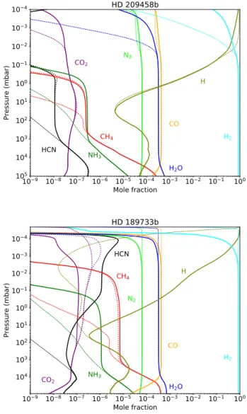
(2011); these profiles were used inVenot et al.(2012) with the original chemical scheme. The stellar and planetary character-istics are the same as in Venot et al. (2012). We used solar elemental abundances (Lodders 2010), but we removed 20% of the oxygen to account for sequestration of oxygen in refractory elements of the deep atmospheric layers. As can be seen in Fig.2, the update of the chemical scheme has a very moderate effect on the chemical composition of these two planets. Whereas quench-ing levels of all species remain the same in HD 209458b, we notice variations in HD 189733b. With V20, CO2 is quenched

about 100 mbar, whereas it was not with V12; the quenching of CH4happens slightly deeper than with V12, indicating that the

chemical lifetime of these species is longer with V20. Although still different, this deeper quenching level of CH4 goes in the

direction of the results found byMoses(2014) for this species. However, important differences are still present for the other species presented in this latter paper (i.e., C2H2, NH3, and HCN).

4.2. Warm Neptunes

We studied the effect of the methanol chemistry update on warm Neptunes, which are more temperate planets than hot Jupiters. We applied our 1D kinetic model alternatively using the two chemical schemes to GJ 436b (see Fig. 3), assuming two dif-ferent metallicities, solar and 100 ˆ solar (100d), as well as to GJ 1214b (see Fig. 4), assuming a metallicity 100d. For both planets, the thermal profiles used are the same as inVenot et al.

(2019), i.e., determined with ATMO (Tremblin et al. 2015) for GJ 436b, and the Generic LMDZ GCM (Charnay et al. 2015) for

10−9 ₁₀−8 ₁₀−7 ₁₀−6 ₁₀−5 ₁₀−4 ₁₀−3 ₁₀−2 ₁₀−1 ₁₀0

Mole frac ion 10−4 10−3 10−2 10−1 100 101 102 103 104 105 Pre ssu re (m ba r) CO2 HCN _NH3CH4 N2 CO H2O H H2

HD 209458b

Mole frac ion 10−4 10−3 10−2 10−1 100 101 102 103 104 Pre ssu re (m ba r) CO2 HCN NH3 CH4 N2 CO H2O H H2

HD 189733b

Fig. 2. Vertical abundances profiles of the main atmospheric con-stituents in two Hot Jupiters: HD 209458b (top) and HD 189733b (bottom). The abundances obtained with the updated chemical scheme (solid lines) are compared to those obtained with the former scheme of

Venot et al.(2012) (dotted lines). Thermochemical equilibrium is shown with thin dash-dotted lines.

GJ 1214b (Fig. 1). For GJ 436b, we assumed a constant eddy diffusion coefficient with altitude, and used two values (108_and

109cm2s´1_{). For GJ 1214b, we used the formula determined by} Charnay et al.(2015), Kzz “ 3 ˆ 107 ˆ P´0.4cm2s´1, with P

in bar. For all the above cases, we observe the same trends: the update of the chemical scheme leads to deeper quenching level, and thus lower abundances for CO, CO2, and HCN. On the

con-trary, but for the same reason, CH4and H2O are found to be more

abundant (Figs.3and 4).

For the model of GJ 436b with a high metallicity, CO and CH4have abundances that are very close in the quenching area.

With a Kzz of 108s cm2s´1, CO is the main C-bearing species

whatever the chemical scheme used, but with a stronger vertical mixing as that presented in Fig.3(i.e., Kzz= 109s cm2s´1), the

main C-bearing species depends on the chemical scheme, i.e., CO with V12 and CH4with V20.

4.3. T Dwarfs: ULAS J1335+11

We modeled a typical T Dwarf ULAS J1335+11 (Leggett et al. 2009) with a thermal profile calculated with ATMO assuming an

10-10 ₁₀-9 ₁₀-8 ₁₀-7 ₁₀-6 ₁₀-5 ₁₀-4 ₁₀-3 ₁₀-2 Mole fraction 10-4 10-3 10-2 10-1 100 101 102 103 104 105 Pre ssu re (m ba r) CO2 HCN NH3 CH4 N2 CO H2O H

GJ 436b nominal - K

= 10

cm

.s

GJ 436b - metallicity 100xsolar - K

= 10

cm

.s

Fig. 3. Same as Fig. 2 for GJ 436b with a solar metallicity and Kzz= 108cm2s´1(top) and with a 100d metallicity and Kzz= 109cm2s´1 (bottom). With the updated chemical scheme, CO sees its abundance decrease.

10

₁₀

₁₀

₁₀

₁₀

₁₀

₁₀

₁₀

₁₀

₁₀

Mole f action

10

10

10

10

10

10

10

10

10

10

P e

ssu

e

(m

ba

)

CO

HCN

NH

CH4

N

CO

H

O

H

H

GJ 1214b - metallicity 100xsolar

Fig. 4. Same as Fig.2for GJ 1214b with a 100d metallicity. As for GJ 436b, with the updated chemical scheme, CO sees its abundance decrease. 10−10 ₁₀−9 ₁₀−8 ₁₀−7 ₁₀−6 ₁₀−5 ₁₀−4 ₁₀−3 ₁₀−2 Mole fraction 10−3 10−2 10−1 100 101 102 103 104 Pre ssu re ( ba r) CO2 HCN NH3 CH4 N2 CO H2O H H2

ULAS J1335+11

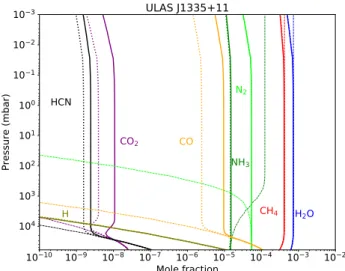
Fig. 5.Same as Fig.2for the brown dwarf ULAS J1335+11.

effective temperature of 500 K and a surface gravity of log (g) = 4 (Fig.1). For the vertical mixing, we assume a constant eddy dif-fusion coefficient of 106 _cm2_s´1_{. Contrary to warm Neptunes,}

we observe that with V20 we obtain more CO and CO2 in the

atmosphere than with the former scheme (see Fig.5) because of the deeper quenching level. The increase in CO abundance is typically of a factor 3 at the effective temperature of late T dwarfs and can impact the CO absorption feature at 4.5 µm (see Sect.6). At higher effective temperatures closer to the L/T transition, we do not observe any important differences between the updated and former scheme, similar to the hot Jupiter cases.

4.4. Uranus and Neptune

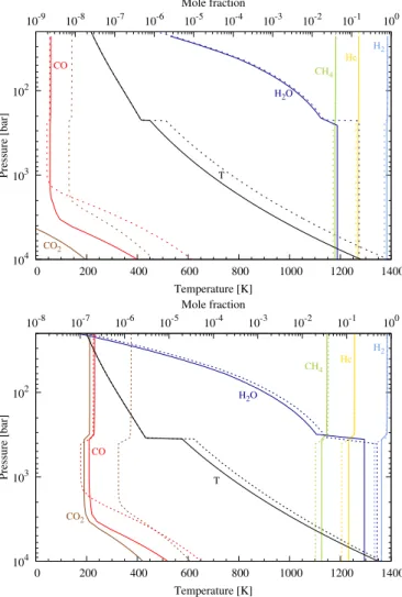
For Uranus and Neptune, the update of the chemical scheme, coupled to the effect of composition on the thermal profile, has a significant effect on the oxygen chemistry. We take the nominal cases ofCavalié et al.(2017) for both planets, i.e., O/H ă 160d (Uranus) and “ 480d (Neptune), a deep Kzz“ 108cm2s´1, an

upper tropospheric CH4mole fraction of 4%, and a “three-layer”

thermal profile. Thus, the model results in upper tropospheric mole fractions of CO of 7.8 ˆ 10´8 _{and 3.8 ˆ 10}´6_{, i.e., 34}

and 19 times, respectively, above model results using the former chemical scheme and above the observed abundances.

This implies that less H2O is required in the layers in which

thermochemical equilibrium prevails to fit the observations of CO. As a consequence the three-layer temperature profiles are colder than in the nominal cases ofCavalié et al.(2017) because the mean molecular weight gradient at the H2O condensation

level is smaller and therefore produces a less sharp temperature increase in this altitude region. The quench level then occurs deeper, enabling more CO to be transported toward the observ-able levels. We find that the upper tropospheric CO can be reproduced in Uranus and Neptune with an O/H of ă45d and 250d. The corresponding model results are shown in Fig.6. The changes induced by the new chemical scheme are slightly more significant for Uranus than for Neptune.

4.5. Summary

The effect of the update depends on the temperature of the quenching level and on the shape of the abundance profiles. On one hand, if quenching happens at a temperature higher than „1500 K and at low pressure (0.1–1 bar, typically what

102 103 104 0 200 400 600 800 1000 1200 1400 10-9 10-8 10-7 10-6 10-5 10-4 10-3 10-2 10-1 100 H₂ He CH₄ H₂O CO₂ CO T Pressure [bar] Temperature [K] Mole fraction 102 103 104 0 200 400 600 800 1000 1200 1400 10-8 10-7 10-6 10-5 10-4 10-3 10-2 10-1 100 H₂ He CH₄ H₂O CO₂ CO T Pressure [bar] Temperature [K] Mole fraction

Fig. 6. Vertical abundances profiles of the main atmospheric con-stituents and oxygen species in Uranus (top) and Neptune (bottom). The abundances obtained with the updated chemical scheme (solid lines), and O/H ă 45 and 250d for Uranus and Neptune (respectively), are compared to those obtained with the former scheme ofVenot et al.

(2012) (dotted lines), with ă160 and 480d for Uranus and Neptune (respectively). The thermal and abundance profiles are thus not obtained with the same boundary conditions (see text for more details).

happens in hot Jupiters atmospheres tested in this work), no sub-stantial changes occur. On another hand, if quenching happens at lower temperature but higher pressure (ą10 bars), then the quenching level is modified, consequently affecting the molec-ular abundances in upper layers. In all the cases we tested, we observe a deeper quenching level with the updated scheme V20. Molecular abundances are affected by the update depending on their slope at the now deeper quench level. If the abundance increases with altitude, the abundance is lowered (e.g., CO and CO2in GJ 436b), and if the abundance decreases with altitude,

the abundance is enhanced (CO in Uranus, Neptune, and ULAS J1335+11).

5. Interpretation of the results

5.1. Zero-dimensional model

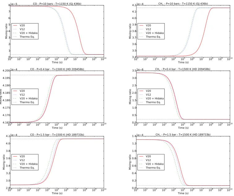
To understand the changes of kinetics and thus of abundances observed in the atmospheres modeled in this paper, we run our 0D model at the pressure and temperature, where CO is quenched in GJ 436b (i.e., 10 bars and 1150 K) and CH4 is

quenched in HD 209458b (i.e., 0.4 bar and 1500 K) and in HD 189733b (i.e., 1.5 bar and 1500 K), with our chemical schemes.

At the level of CO quenching in GJ 436b (Fig.7), we observe that the kinetics of CO and CH4are much slower with V20 than

with V12. The difference is of two orders of magnitude. We iden-tify that this slowdown in the updated scheme is due to the “non-presence” of the reaction CH3OH ` H é CH3` H2O, which is

included in the scheme of V12 with the reaction rate proposed byHidaka et al.(1989). Adding this unique reaction to our new chemical scheme (hereafter V20+Hidaka) accelerates the kinet-ics of CH4and CO (see Fig.7, top) and brings the abundances

of CO (as well as CO2and HCN) in the 1D model very close to

that found with V12 (Fig.8). The difference of CO abundance at 100 mbar is reduced from 7 ppm to 1 ppm (i.e., a factor 2.8 and 1.1 respectively). We note that the change in CO2abundance is

due to the Hidaka reaction for pressures greater than 1 bar, but also to the reaction CO ` OH é CO2` H for lower pressures.

On the other side, at the levels of CH4 quenching in

HD 209458b and in HD 189733b (Fig.7, middle and bottom), there is only a minor difference (less than a factor 2) concern-ing the kinetics of CO and CH4in V12 and V20. This explains

why we obtain (almost) the same chemical composition for these planets with both chemical schemes. Also, adding Hidaka’s reac-tion to V20 slightly accelerates the kinetics of CO and CH4, but

the variation remains small at about a factor „2. We can also note that the kinetics of V20+Hidaka is in reality further away from V12 than V20. This excessive acceleration explains the 1D abundance profiles of methane determined for these plan-ets (Fig. 8). CH4 quenches at (slightly) higher altitude when

Hidaka’s reaction is included than with the original V20, even higher than what is obtained with V12. For HD 209458b, the deviation of CH4abundance at 100 mbar between V12 and V20

is of 4.5 ppb, whereas the gap between V12 and V20+Hidaka is about 20 ppb. These differences are really small, i.e., a factor 1.02 and 1.09, respectively. In the case of CH4 in HD 189733b

(at 10 mbar), the difference between V12 and V20 is a little more important (1 ppm, i.e., a factor 1.2) than the gap between V12 and V20+Hidaka (0.6 ppm, i.e., a factor 1.1). However, com-pared to the factor 2.8 of deviation observed for CO in GJ 436b, all the differences of CH4 abundances in hot Jupiters remain

really minor. In this case of HD 189733b, it is interesting to compare the methane abundances obtained with those found in

Moses(2014). This paper focuses on HD 189733b and compares the atmospheric abundances of several species, including CH4,

obtained using V12 and theMoses et al.(2011) chemical scheme. At 10 mbar, CH4 has an abundance of „10´5 with the Moses et al. (2011) scheme, and „6 ˆ 10´6 _{with V12 (like in this}

study). The update of the scheme we perform in this work leads indeed to an increase of CH4abundance (to 7 ˆ 10´6); thus this

update is toward the result obtained with theMoses et al.(2011) scheme, but the new value we derive remains lower and is still closer to the previous value obtained with V12.

Finally, we can say that the reaction CH3OH ` H é

CH3` H2O with the reaction rate ofHidaka et al.(1989), does

have a role in the chemical composition of hot Jupiters, but the amplitude of variation generated by the addition of this single reaction in the new V20 scheme remains very small and is not crucial for the kinetics of conversion of CO/CH4.

5.2. Chemical pathways

To understand the differences between the different panels of Figs.7and8, and thus why the update of the chemical scheme

100 ₁₀1 ₁₀2 ₁₀3 ₁₀4 ₁₀5 ₁₀6 ₁₀7 ₁₀8 ₁₀9 ₁₀10 Time (s) 0 1 2 3 4 5 6 7 8 Mixing ratio 1e 5 CO - P=10 bars - T=1150 K (GJ 436b) V20 V12 V20 + Hidaka Thermo Eq. 100 ₁₀1 ₁₀2 ₁₀3 ₁₀4 ₁₀5 ₁₀6 ₁₀7 ₁₀8 ₁₀9 ₁₀10 Time (s) 3.4 3.5 3.6 3.7 3.8 3.9 4.0 4.1 4.2 Mixing ratio 1e 4 CH4 - P=10 bars - T=1150 K (GJ 436b) V20 V12 V20 + Hidaka Thermo Eq. 100 ₁₀1 ₁₀2 ₁₀3 ₁₀4 ₁₀5 ₁₀6 ₁₀7 ₁₀8 ₁₀9 ₁₀10 Time (s) 4.165 4.170 4.175 4.180 4.185 4.190 4.195 4.200 Mixing ratio 1e 4 CO - P=0.4 bar - T=1500 K (HD 209458b) V20 V12 V20 + Hidaka Thermo Eq. 100 ₁₀1 ₁₀2 ₁₀3 ₁₀4 ₁₀5 ₁₀6 ₁₀7 ₁₀8 ₁₀9 ₁₀10 Time (s) 0.0 0.5 1.0 1.5 2.0 2.5 3.0 3.5 Mixing ratio 1e 6 CH4 - P=0.4 bar - T=1500 K (HD 209458b) V20 V12 V20 + Hidaka Thermo Eq. 100 ₁₀1 ₁₀2 ₁₀3 ₁₀4 ₁₀5 ₁₀6 ₁₀7 ₁₀8 ₁₀9 ₁₀10 Time (s) 2.8 3.0 3.2 3.4 3.6 3.8 4.0 4.2 Mixing ratio 1e 4 CO - P=1.5 bar - T=1500 K (HD 189733b) V20 V12 V20 + Hidaka Thermo Eq. 100 ₁₀1 ₁₀2 ₁₀3 ₁₀4 ₁₀5 ₁₀6 ₁₀7 ₁₀8 ₁₀9 ₁₀10 Time (s) 0.0 0.2 0.4 0.6 0.8 1.0 1.2 1.4 Mixing ratio 1e 4 CH4 - P=1.5 bar - T=1500 K (HD 189733b) V20 V12 V20 + Hidaka Thermo Eq.

Fig. 7.Temporal evolution of the abundance of CO (left) and CH4(right) at their quenching levels in GJ 436b (top), HD 209458b (middle), and HD 189733b (bottom). The corresponding pressures and temperatures are indicated on each panel. The abundances obtained with the updated chemical scheme (solid red lines) are compared to those obtained with the former scheme ofVenot et al.(2012) (dotted blue lines), to the updated chemical scheme to which has been added Hidaka’s reaction (dot-dashed green lines) and to the thermochemical equilibrium at these conditions of P and T (dotted black lines). The initial conditions are the thermochemical abundances (assuming solar elemental abundances) at 1 bar and 1100 K (for GJ 436b), at 3.5 bars and 1750 K (for HD 209458b), and at 13 bars and 1570 K (for HD 189733b).

significantly modifies the atmospheric composition of warm Neptunes, T dwarfs, giant planets, but not hot Jupiters, we ana-lyzed the chemical pathways occurring in the different P–T conditions. We found that the behavior of the hydrogen radical is the key to explaining the differences.

At 10 bars and 1150 K (i.e., CO quenching level in GJ 436b), whatever the chemical scheme, the net production rate of H is positive. The kinetic analysis of V12 scheme is represented in Fig.9. The hydrogen radical comes mainly from metathesis (H-transfer reactions) between H2 and another radical (R(.));

75% of H reacts with CO to form HCO, which then reacts mainly with H to give formaldehyde (H2CO). Then, by addition

of H again, H2CO forms either the CH2OH or CH3O radical.

These two species, by metathesis, are transformed into methanol; 10% of the hydrogen present in the atmosphere reacts with the formed methanol, through Hidaka’s reaction CH3OH + H ÝÑ

CH3 + H2O, to form the methyl radical. CH3 then reacts with

H or H2 to create CH4. In this P–T condition, with this

chem-ical scheme, 30% of CH3 comes from Hidaka’s reaction. This

reaction is thus very important in this context.

We performed the same analysis with the updated scheme (Fig. 10). The production of methanol from H2 is identical to

that of V12. Then, because Hidaka’s reaction is not included in this scheme, H cannot react with CH3OH to form CH3. In

V20 scheme, only 5% of CH3 comes from methanol, through

the priming reaction CH3OH (+M) ÝÑ CH3 + OH (+M). The

majority of methyl radical comes from the initiation reactions of methane (CH4(+M) ÝÑ CH3+ H) and ethane (C2H6(+M) ÝÑ

CH3 (+M)). Also, CH3 then reacts with H or H2 to create

CH4. We see that the main difference between the two

chemi-cal schemes is due to the chemichemi-cal pathways between CH3OH

and CH3.

We performed the same analysis at 0.4 bar and 1500 K, i.e., CH4 quenching level in HD 209458b. We find that the main

10-7 ₁₀-6 ₁₀-5 ₁₀-4 Mole fraction 10-4 10-3 10-2 10-1 100 101 102 103 104 105 Pressure (mbar) CO GJ 436b nominal - Kzz = 108 cm2.s−1 New Methanol V12

New Methanol + Hidaka Thermo Eq. 10-6 ₁₀-5 ₁₀-4 Mole fraction 10-4 10-3 10-2 10-1 100 101 102 103 104 Pressure (mbar) CH4 HD 189733b New Methanol V12

New Methanol + Hidaka Thermo Eq. 10-8 ₁₀-7 ₁₀-6 ₁₀-5 ₁₀-4 Mole fraction 10-4 10-3 10-2 10-1 100 101 102 103 104 105 Pressure (mbar) CH4 HD 209458b New Methanol V12

New Methanol + Hidaka Thermo Eq.

Fig. 8.Vertical abundances profiles of CO in GJ 436b (top) and of CH4 in HD 189733b (middle) and in HD 209458b (bottom) using different chemical schemes, as labeled.

chemical pathways are the same with the two chemical schemes. Contrary to the previous case, at this lower pressure, the net production rate of H is negative (i.e., positive loss rate). The majority of hydrogen (90%) is equally consumed to give H2,

Chemical pathways in V12

{

Fig. 9. Chemical pathways controlling H Ø CH4 conversion in the chemical scheme ofVenot et al.(2012) at 10 bars and 1150 K.

Chemical pathways in V20 (this study)

R(.) + H2 H(.) + RH CH3OH CH4 (.)CH3 + CO (.)HCO H2CO CH3O(.) (.)CH2OH +H(.) +H(.) 5%

{

Fig. 10. Chemical pathways controlling H Ø CH4 conversion in the updated chemical scheme at 10 bars and 1150 K.

CH3, and CH4. The remaining 10% are involved in the following

loop:

H ` CO ÝÑ HCO HCO ` H ÝÑ CO ` H2.

Our analysis shows that at this pressure and temperature, Hidaka’s reaction does not step into the overall produc-tion/destruction of CH4, CH3, and CO, which leads to identical

results between the two schemes.

The same analysis has been performed for the quenching level in HD 189733b and leads to the same global conclusion than in HD 209458b. However at this pressure and temperature (1.5 bar and 1500 K), Hidaka’s reaction plays a minor role in V12: 0.1% of CH3is produced through this reaction (versus 0%

and 30% in the cases of HD 209458b and GJ 436b, respectively), which explains why there is a larger difference between V12 and V20 for HD 189733b than for HD 209458b.

To summarise, the key to explaining our results is the pro-duction rate of hydrogen. In a P–T domain where the propro-duction rate of H is positive, Hidaka’s reaction plays a major role in V12 and thus there will be differences between the two schemes. In contrast, in a P–T domain where the loss rate of H is positive, then Hidaka’s reaction does not play its rate-accelerating effect and results obtained with the two schemes are very similar.

6. Discussion

6.1. Implications for hot Jupiters

The update of the chemical scheme does not fundamentally impact the predicted atmospheric composition of HD 209458b and HD 189733b, which can be considered as typical hot Jupiters with a solar elemental composition. The main variation of abundance is the decrease of CO2 in the upper atmosphere of

HD 189733b. We calculated the synthetic transmission spec-tra of this planet with the forward model TauRex (Waldmann et al. 2015a,b) and observed only a slight variation in the CO2

absorption band at 4–5 µm (50 ppm). This difference would hardly be distinguishable with future observations performed with James Webb Space Telescope (JWST)/Near-Infrared Spec-trograph (NIRSpec) or Atmospheric Remote-sensing Infrared Exoplanet Large-survey (ARIEL), with at least one single obser-vation. Stacking together several transits data reduces the error bars, eventually making the distinction possible (Mugnai et al. 2019). Because the abundance of CO2 is dependent on the

quenching level in HD 189733b, an accurate estimation of its abundance could help to constrain and better understand the mixing occurring in the atmospheres of hot Jupiters.

We confirm the abundances of NH3, HCN, CH4, and C2H2

obtained in Venot et al. (2012) with the previous chemical scheme. Although in the atmosphere of HD 189733b quench-ing of CH4 happens deeper than with V12 (leading to a very

small increase of the abundance of this species), the other afore-mentioned species are not affected by the update of the scheme. Thus, our global results are not modified in a way that would bring them closer to the results obtained byMoses(2014). As we explained in Sect. 5, in the atmospheres of hot Jupiters, the differences between our results and those of Moses(2014) are thus not only due to the choice of the reaction rate of CH3OH ` H é CH3` H2O. This result comforts us with the

idea that a global validation of a scheme prevails compared to individual reaction calculations.

6.2. Implications for warm Neptunes

The update of the chemical scheme has important consequences on the molecular composition of warm Neptunes, especially for atmospheres with high metallicities. Because the quenching level of CO2, CO, and CH4is modified, the abundances of these

species vary and even a change of the main C-bearing species can occur (Fig.3). The change of chemical composition found for warm Neptunes has observational consequences.

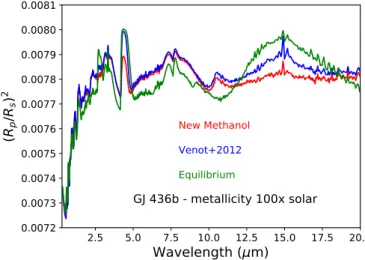
With the forward model TauRex, we computed the synthetic transmission spectra for our models of GJ 436b with a high metallicity. We calculated the spectra corresponding to the com-positions at equilibrium, determined with V12 and the updated scheme (Fig.11). First, we note the important variations between the disequilibrium spectra and those at equilibrium between 1 and 10 µm and in NH3band (11 µm), which are the result of the

high NH3 abundance in disequilibrium models. The important

departures in CO2band (15 µm) result from the high abundance

of CO2at low pressure in the equilibrium model. We can expect

that future high-resolution observations of warm Neptunes such as GJ 436b could be able to detect the possible disequilibrium composition of these planets, even if cloudy (Kawashima et al. 2019), and would certainly help to constrain the vertical mix-ing responsible of quenched abundances. Then, between the two disequilibrium spectra, important variations are visible in CO2absorption bands (4–5 µm, 15 µm). As this species is less

2.5 5.0 7.5 10.0 12.5 15.0 17.5 20.0 Wavelength

(

m)

0.0072

0.0073

0.0074

0.0075

0.0076

0.0077

0.0078

0.0079

0.0080

0.0081

(

/

)

GJ 436b - metallicity 100x solar

New Methanol

Venot+2012

Equilibrium

Fig. 11.Synthetic transmission spectra of GJ 436b’s atmosphere with a metallicity 100d. The different spectra correspond to the compositions at chemical equilibrium (green), and with disequilibrium compositions (Kzz= 109cm2s´1) calculated with theVenot et al.(2012) scheme (blue), and with the updated scheme (red). The spectral resolving power is 300.

abundant with the updated scheme, the absorption is lower in these bands, resulting in a lower pRp{Rsq2. Such a departure (up

to 100 ppm) will be easily observable with future instruments such as JWST/MIRI (Mid-Infrared Instrument). Thus, the choice of the chemical scheme is critical for an accurate constraint on vertical mixing.

6.3. Implications for brown dwarfs

The updated scheme has a significant impact on the abundance of CO in late T dwarfs. This has a direct impact on the planet spectrum in the 4.7 µm window because CO is a strong absorber at these wavelengths. We show in Fig. 12 the emission spec-trum at equilibrium with the former and the updated scheme. The new scheme can lead up to a factor 2 decrease in the flux in this window because of the increase of the CO abundance. Such a difference will be easily constrained by JWST/NIRSpec measurements. The updated scheme combined with JWST mea-surements will therefore allow us to better characterize the strength of vertical mixing that is necessary to reproduce the out-of-equilibrium abundance of CO in cold brown dwarfs. 6.4. Implications for the formation of Uranus and Neptune The results obtained for Uranus and Neptune in this paper with the thermochemical model ofVenot et al.(2012) and the updated chemical scheme for methanol do not waive the difference found more than two decades ago between the two planets in terms of deep oxygen abundance. This difference primarily results from their different tropospheric CO abundances. WhileTeanby et al.

(2019) recently propose from their Herschel-SPIRE data a model without any tropospheric CO in Neptune, i.e., very similar to Uranus, their results probably lack sensitivity in the upper tropo-sphere to make this result robust.Moreno et al.(2011) show in a preliminary combined analysis of Herschel-SPIRE and IRAM-30 m data, including the CO(1–0) line that is most sensitive to the tropospheric CO, that the tropospheric CO in Neptune was 0.20 ˘ 0.05 ppm.

Assuming the CO abundance difference between the two planets is representative of their respective deep oxygen abun-dances, and according to our new results, only Neptune could

1 2 3 4 5 6 Wavelength

(

m)

Sp

ec

tra

l fl

ux

(W

.

−2

.

−1

)

ULAS J1335+11

New Methanol

Venot+2012

Equilibrium

Fig. 12.Emission spectra for ULAS J1335+11 (for R = 0.1 Rdat 10 pc) obtained with the updated chemical scheme (red), compared with those obtained with the former scheme ofVenot et al.(2012) (blue) and with equilibrium chemistry (green).

in principle have formed from ices condensed in clathrates (C/O „ 0.12). On the other hand, the low upper limit on O/H for Uranus is in contradiction with such a process (C/O „ 1). Inter-estingly however, this upper limit is close to the C/H required to fit CH4 (10.383 dex versus 10.331 dex, respectively), which

is one of the conditions under which Uranus planetesimal ices could have formed on the CO snow line and be mainly composed of CO rather than H2O (Ali-Dib et al. 2014). Such a low upper

limit may also be derived from inhibited convection in the deep layers of Uranus precluding any tropospheric abundance mea-surements to be representative of the bulk composition of the planet. We should however not forget that several model param-eters remain uncertain such as the deep Kzz. A lower Kzz than

that assumed in our nominal models would result in higher O/H (Cavalié et al. 2017) and therefore change our interpretation.

7. Conclusions

We present in this paper an update of the chemical scheme of Venot et al. (2012). The analysis of Moses (2014) denotes that discrepancies between her results and Venot et al.(2012) could be due to differences in chemical rates involving methanol. This has motivated us to update the Venot et al.(2012) chem-ical network by replacing their methanol sub-network by that put together byBurke et al.(2016), following a comprehensive study on methanol combustion. We validated this new net-work against experimental measurements. We emphasize that one change, among others, in our new chemical network is that the controversial reaction CH3OH`HéCH3`H2O has been

removed.

The new updated scheme V20 gives very similar results to the former scheme for hot Jupiters. A variation of CO2

abun-dance is observed in HD 189733b atmosphere, but only modifies the synthetic spectra to a lower extent (50 ppm at 4–5 µm). A very small change of CH4quenching level, which slightly

mod-ifies in return the abundance of this species, is also observed in HD 189733b, without any impact on the observable.

For warm Neptunes and T Dwarfs, the update has more significant implications because the reaction CH3OH `

H é CH3` H2 played an important role in the former scheme

of V12. Owing to the quenching of CO, CO2 (and eventually

H2O and CH4in high metallicity atmospheres) happening deeper

with the new scheme, the abundances of these species are modi-fied compared to the results obtained with theVenot et al.(2012) chemical scheme. The change is important enough to affect the synthetic spectra. The differences with the former scheme (up to 100 ppm in transmission for warm Neptune and a factor 2 in emission for the T Dwarf) will certainly be detectable with future instruments such as JWST. Using an accurate and updated chemical scheme is thus paramount for a correct interpretation of future observations and for a better comprehension of mixing processes at play in these atmospheres.

The consequence of the update is also fundamental for our understanding of the formation of Uranus and Neptune. For a given O/H ratio, the abundance of CO is higher with the updated scheme than with the former scheme. Consequently, the O/H ratios necessary to reproduce the tropospheric observations of CO are lower than what had been previously found. The updated scheme indicates O/H of ă45 and 250d for Uranus and Neptune, respectively.

Finally, we derived a reduced chemical scheme from this update, for future 3D kinetic models that are crucial (and the next step) for our understanding of (exo)planetary atmospheres. The next steps on the improvement of our chemical scheme will imply adding new species, such as sulphur species, following the recent detection of H2S in Uranus and Neptune (Irwin et al. 2018, 2019). Phosphorus species could also be of interest to extend the scope of our work, as PH3 can provide additional constraints

on the deep oxygen abundance (Visscher & Fegley 2005). The use of this species as a tracer for O abundance will be possi-ble only if PH3is quenched in the atmospheres of giant planets,

which is an expected behavior of this moleculeFegley & Lodders

(1994);Visscher et al.(2006). However, PH3remains undetected

in Uranus and Neptune (Moreno et al. 2009). Although these species have not been detected yet in exoplanet atmospheres, their presence is expected and it has been shown that they should be observable with JWST (Baudino et al. 2017;Wang et al. 2017). We show with this study that collaborations between astro-physicists and combustion specialists are fruitful in order to accurately study high-temperature atmospheres. The intensive work performed in the field of combustion is paramount to perform reliable atmospheric modeling, leading to a correct interpretation of observations.

Acknowledgements.The author thanks the anonymous referee for his/her care-ful review that helps improving the manuscript. O.V. and T.C. thank the CNRS/INSU Programme National de Planétologie (PNP) and CNES for funding support. P.T. acknowledges support from the European Research Council (grant no. 757858 – ATMO). The authors thank B. Edwards, Q. Changeat, I. Waldmann for useful discussions on JWST and ARIEL observations.

References

Akrich, R., Vovelle, C., & Delbourgo, R. 1978,Combust. Flame, 32, 171 Ali-Dib, M., Mousis, O., Petit, J.-M., & Lunine, J. I. 2014,ApJ, 793, 9 Alzueta, M. U., Bilbao, R., & Finestra, M. 2001,Energy Fuels, 15, 724 Aniolek, K. W., & Wilk, R. D. 1995,Energy Fuels, 9, 395

Aranda, V., Christensen, J. M., Alzueta, M. U., et al. 2013,Int. J. Chem. Kinet., 45, 283

Aronowitz, D., Santoro, R., Dryer, F., & Glassman, I. 1979,Symp. Int. Combust., 17, 633

Arridge, C. S., Agnor, C. B., André, N., et al. 2012,Exp. Astron., 33, 753 Arridge, C. S., Achilleos, N., Agarwal, J., et al. 2014,Planet. Space Sci., 104, 122 Atreya, S. K., Wong, M. H., Owen, T. C., et al. 1999,Planet. Space Sci., 47, 1243 Barbe, P., Battin-Leclerc, F., & Côme, G. M. 1995,J. Chim. Phys., 92, 1666 Baudino, J.-L., Mollière, P., Venot, O., et al. 2017,ApJ, 850, 150

Bowman, C. T. 1975,Combust. Flame, 25, 343

Burke, U., Metcalfe, W. K., Burke, S. M., et al. 2016,Combust. Flame, 165, 125 Cathonnet, M., Boettner, J. C., & James, H. 1982,J. Chim. Phys., 79, 475 Cavalié, T., Billebaud, F., Dobrijevic, M., et al. 2009,Icarus, 203, 531 Cavalié, T., Moreno, R., Lellouch, E., et al. 2014,A&A, 562, A33 Cavalié, T., Venot, O., Selsis, F., et al. 2017,Icarus, 291, 1 Charnay, B., Meadows, V., & Leconte, J. 2015,ApJ, 813, 15 Chen, J.-Y. 1991,Combust. Sci. Technol., 78, 127

Cooke, D. F., Dodson, M. G., & Williams, A. 1971,Combust. Flame, 16, 233 Cribb, P. H., Dove, J. E., & Yamazaki, S. 1984, in20th Symp. Int. Combust.,

6779

Dayma, G., Ali, K. H., & Dagaut, P. 2007,Proc. Combust. Inst., 31, 411 de Pater, I., & Richmond, M. 1989,Icarus, 80, 1

de Pater, I., Romani, P. N., & Atreya, S. K. 1991,Icarus, 91, 220

Egolfopoulos, F. N., Du, D. X., & Law, C. K. 1992,Combust. Sci. Technol., 83, 33

Fegley, B. J., & Lodders, K. 1994,Icarus, 110, 117

Fieweger, K., Blumenthal, R., & Adomeit, G. 1997,Combust. Flame, 109, 599 Gautier, D., & Hersant, F. 2005,Space Sci. Rev., 116, 25

Gilbert, R. G., Luther, K., & Troe, J. 1983,Ber. Bunsenges. Phys. Chem., 87, 169 Griffith, C. 2000,ASP Conf. Ser., 212, 142

Grotheer, H.-H., Kelm, S., Driver, H. S. T., et al. 1992,Phys. Chem. Chem. Phys., 96, 1360

Held, T., & Dryer, F. 1994,Symp. Int. Combust, 25, 901 Held, T. J., & Dryer, F. L. 1998,Int. J. Chem. Kinet., 30, 805

Hidaka, Y., Oki, T., Kawano, H., & Higashihara, T. 1989,J. Phys. Chem., 93, 7134

Ing, W. C., Sheng, C. Y., & Bozzelli, J. W. 2003,Fuel Process. Technol., 83, 111 Irwin, P. G. J., Toledo, D., Garland, R., et al. 2018,Nat. Astron., 2, 420 Irwin, P. G. J., Toledo, D., Garland, R., et al. 2019,Icarus, 321, 550 Kawashima, Y., Hu, R., & Ikoma, M. 2019,ApJ, 876, L5 Kumar, K., & Sung, C.-J. 2011,Int. J. Chem. Kinet., 43, 175

Leggett, S. K., Cushing, M. C., Saumon, D., et al. 2009,ApJ, 695, 1517 Li, J., Zhao, Z., Kazakov, A., et al. 2007,Int. J. Chem. Kinet., 39, 109 Li, C., Oyafuso, F. A., Brown, S. T., et al. 2018,AGU Fall Meeting Abstracts,

2018, P33F

Liao, S. Y., Jiang, D. M., Huang, Z. H., & Zeng, K. 2006,Fuel, 85, 1346 Lindemann, F. A., Arrhenius, S., Langmuir, I., et al. 1922,Trans. Faraday Soc.,

17, 598

Lindstedt, R. P., & Meyer, M. P. 2002,Proc. Combust. Inst., 29, 1395

Lodders, K. 2010, in Principles and Perspectives in Cosmochemistry, eds. A. Goswami, & B. E. Reddy (Berlin, Heidelberg: Springer Berlin Heidel-berg), 379

Lodders, K., & Fegley, Jr. B. 1994,Icarus, 112, 368 Luszcz-Cook, S. H., & de Pater, I. 2013,Icarus, 222, 379

Madhusudhan, N., Agúndez, M., Moses, J. I., & Hu, Y. 2016,Space Sci. Rev., 205, 285

Metghalchi, M., & Keck, J. C. 1982,Combust. Flame, 48, 191

Moreno, R., Marten, A., & Lellouch, E. 2009, AAS/Division for Planetary Sciences Meeting Abstracts, 41, 28.02

Moreno, R., Lellouch, E., Courtin, R., et al. 2011,Geophys. Res. Abstracts, 13, 8299

Moses, J. I. 2014,Phil. Trans. R. Soc. London Ser. A, 372, 20130073 Moses, J. I., Visscher, C., Fortney, J. J., et al. 2011,ApJ, 737, 15

Mousis, O., Fletcher, L. N., Lebreton, J.-P., et al. 2014,Planet. Space Sci., 104, 29

Mousis, O., Atkinson, D. H., Spilker, T., et al. 2016,Planet. Space Sci., 130, 80 Mousis, O., Atkinson, D. H., Cavalié, T., et al. 2018,Planet. Space Sci., 155, 12 Mugnai, L., Edwards, B., Papageorgiou, A., Pascale, E., & Sarkar, S. 2019,Eur.

Planet. Sci. Congress, 2019, 270

Natarajan, K., & Bhaskaran, K. A. 1981,Combust. Flame, 43, 35

Noorani, K. E., Akih-Kumgeh, B., & Bergthorson, J. M. 2010,Energy & Fuels, 24, 5834

Norton, T., & Dryer, F. 1989,Combust. Sci. Technol., 63, 107 Owen, T., Mahaffy, P., Niemann, H. B., et al. 1999,Nature, 402, 269 Pollack, J. B., Hubickyj, O., Bodenheimer, P., et al. 1996,Icarus, 124, 62 Rasmussen, C. L., Wassard, K. H., Dam-Johansen, K., & Glarborg, P. 2008,Int.

J. Chem. Kinet., 40, 423

Ren, W., Dames, E., Hyland, D., Davidson, D., & Hanson, R. 2013,Combust. Flame, 160, 2669

Stewart, P., Larson, C., & Golden, D. 1989,Combust. Flame, 75, 25 Teanby, N. A., Irwin, P. G. J., & Moses, J. I. 2019,Icarus, 319, 86 Tremblin, P., Amundsen, D. S., Mourier, P., et al. 2015,ApJ, 804, L17 Tsuboi, T., & Hashimoto, K. 1981,Combust. Flame, 42, 61

Veloo, P. S., Wang, Y. L., Egolfopoulos, F. N., & Westbrook, C. K. 2010, Combust. Flame, 157, 1989

Venot, O., Hébrard, E., Agúndez, M., et al. 2012,A&A, 546, A43 Venot, O., Bounaceur, R., Dobrijevic, M., et al. 2019,A&A, 624, A58 Visscher, C., & Fegley, Jr. B. 2005,ApJ, 623, 1221

Visscher, C., Lodders, K., & Fegley, B. J. 2006,ApJ, 648, 1181 Visscher, C., Moses, J. I., & Saslow, S. A. 2010,Icarus, 209, 602 Wakelam, V., Herbst, E., Loison, J. C., et al. 2012,ApJS, 199, 21 Waldmann, I. P., Tinetti, G., Rocchetto, M., et al. 2015a,ApJ, 802, 107 Waldmann, I. P., Rocchetto, M., Tinetti, G., et al. 2015b,ApJ, 813, 13 Wang, D., Lunine, J. I., & Mousis, O. 2016,Icarus, 276, 21 Wang, D., Miguel, Y., & Lunine, J. 2017,ApJ, 850, 199

Westbrook, C. K., & Dryer, F. L. 1979,Combust. Sci. Technol., 20, 125 Wong, M. H., Mahaffy, P. R., Atreya, S. K., Niemann, H. B., & Owen, T. C.

2004,Icarus, 171, 153

Appendix A: Short review of methanol combustion experimental studies

Table A.1. Overview of the main studies published over the 50 past year on the pyrolysis of methanol.

Reference Reactor Temperature range (K) Pressure Equivalence ratio

Cooke et al.(1971) A 1570–1879 1 atm 1.00

Bowman(1975) A 1545–2180 0.18–0.46 MPa 0.375–6.0

Akrich et al.(1978) F 298 0.11 atm 0.77–1.53

Aronowitz et al.(1979) B 1070–1225 0.1 MPa 0.03–3.16

Westbrook & Dryer(1979) A-B 1000–2180 0.1–0.5 MPa 0.05–3.0

Tsuboi & Hashimoto(1981) A 1200–1800 0.2–2.0

Natarajan & Bhaskaran(1981) A 1300–1700 0.25–0.45 MPa 0.5–1.5

Cathonnet et al.(1982) D 700–900 0.02–0.05 MPa 0.5–4.0

Metghalchi & Keck(1982) F 300–500 0.1 MPa 0.5–1.4

Yano & Ito(1983) C 700–1000

Cribb et al.(1984) A 2000 0.04 MPa

Hidaka et al.(1989) A 1372–1842

Norton & Dryer(1989) B 1025–1090 0.1 MPa 0.6–1.6

Chen(1991) D

Egolfopoulos et al.(1992) A-B-E-F 820–2180 0.005–0.47 MPa 0.05

Grotheer et al.(1992) C-F

Held & Dryer(1994) B 810–1043 1–10 atm 0.60–1.60

Aniolek & Wilk(1995) D 650–700 0.92 atm 0.50–1.50

Fieweger et al.(1997) A 800–1200 12.83–39.48 atm 1.00

Held & Dryer(1998) A-B-E-F 633–2050 0.026–2 MPa 0.05–2.6

Alzueta et al.(2001) B 700–1500 1 atm 0.07–2.70

Lindstedt & Meyer(2002) A-B-F

Ing et al.(2003) B 873–1073 1–5 atm 0.75–1.00

Ing et al.(2003) B 1073 1–10 atm

Rasmussen et al.(2008) B 650–1350 1.00 atm 0.004–0.08

Liao et al.(2006) D 300-550 0.1 MPa 0.6–1.4

Dayma et al.(2007) D 700–1090 10 atm 0.30–1.00

Li et al.(2007) A-B-F 300–2200 0.1–2 MPa 0.05–6.0

Noorani et al.(2010) A 1068–1776 2–12 atm 0.50–2.00

Veloo et al.(2010) C 343 1 atm 0.70–1.50

Kumar & Sung(2011) C 850–1100 6.91–29.61 atm 0.25–1.00

Aranda et al.(2013) B 600–900 20–100 atm 4.35–0.06

Ren et al.(2013) A 1200–1650 0.1–0.3 MPa

Burke et al.(2016) A-C 820–1650 0.2–5 MPa 0.5–2.0

Notes. Reactor types are as follows: shock tube (A), plug flow reactor (B), rapid compression machine (C), stirred reactor (D), static reactor (E), premixed flame (F).

TableA.1gives an overview of the main studies published over the 50 past years on the pyrolysis of methanol. The CH3OH

sub-network from Burke et al.(2016) that we implemented in our model results from these studies.

Appendix B: New CH3OH sub-scheme and

reactions with a logarithmic dependence in pressure

Under certain conditions, some reaction rate expressions depend on pressure as well as temperature. Generally speaking, the rate for unimolecular/recombination fall-off reactions increases with increasing pressure, while the rate for chemically activated bimolecular reactions decreases with increasing pressure. Sev-eral expressions are available in the literature to express the variation of the kinetic data between high and low pressure limit. The Lindemann approach (Lindemann et al. 1922), the Troe form (Gilbert et al. 1983), or the approach taken at SRI International

by Stewart et al. (1989) are the main expressions commonly used for the pressure-dependent reactions. The sub-mechanism of methanol combustion uses another kind of expression for the pressure dependence using logarithmic interpolation with the key word PLOG. Miller & Lutz (2003, priv. comm.) developed a generalised method for describing the pressure dependence of a reaction rate based on direct interpolation of reaction rates spec-ified at individual pressures. In this formulation, the reaction rate is described in terms of the standard modified Arrhenius rate parameters. Different rate parameters are given for discrete pressures within the pressure range of interest. When the actual reaction rate is computed, the rate parameters are determined through logarithmic interpolation of the specified rate constants at the current pressure from the simulation. This approach pro-vides a very straightforward way for users to include rate data from more than one pressure regime.

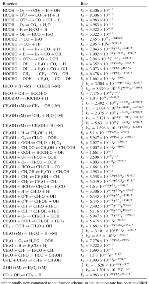
TableB.1lists the reactions of the new methanol sub-scheme we include in our kinetic model. We list in Table B.2 the

Table B.1. Reactions of the new chemical sub-network of CH3OH not involving a logarithmic dependence with pressure, extracted fromBurke et al.(2016). Reaction Rate HCOH ` O2ÝÑ CO2` H ` OH k0“ 8.306 ˆ 10´12 HCOH ` O3_{P ÝÑ CO} 2` H ` H k0“ 8.306 ˆ 10´11 HCOH ` O3<sub>P ÝÑ CO ` OH ` H k</sub> 0“ 4.983 ˆ 10´11 HCOH ` O2é CO2` H2O k0“ 4.983 ˆ 10´11 HCOH ` H é H2CO ` H k0“ 3.322 ˆ 10´10 HCOH ` OH é HCO ` H2O k0“ 3.322 ˆ 10´11 HOCHO é CO ` H2O k0“ 2.45 ˆ 1012e´30400{T HOCHO é CO2` H2 k0“ 2.95 ˆ 109e´24390{T HOCHO ` H ÝÑ H2` CO2` H k0“ 7.043 ˆ 10´18T2.1e´2447{T HOCHO ` H ÝÑ H2` CO ` OH k0“ 1.002 ˆ 10´10T´0.35e´1502{T HOCHO ` O3<sub>P ÝÑ CO ` 2 OH k</sub> 0“ 2.94 ˆ 10´6T´1.9e´1496{T HOCHO ` OH ÝÑ H2O ` CO2` H k0“ 4.352 ˆ 10´18T2.06e´460.5{T HOCHO ` OH ÝÑ H2O ` CO ` OH k0“ 3.073 ˆ 10´17T1.51e483.7{T HOCHO ` CH3ÝÑ CH4` CO ` OH k0“ 6.478 ˆ 10´31T5.8e´1106{T HOCHO ` OOH ÝÑ H2O2` CO ` OH k0“ 1.661 ˆ 10´12e´5993{T H2CO ` H (+M) é CH2OH (+M) " k0“ 3.504 ˆ 10´16T´4.82e´3283{T k8“ 8.970 ˆ 10´13T0.454e´1810{T H2CO ` OH é HOCH2O k0“ 7.475 ˆ 10´9T´1.1 HOCH2O é HOCHO ` H k0“ 1.0 ˆ 1014e´7491{T CH3OH (+M) é CH3` OH (+M) " k0“ 2.492 ˆ 1019T´6.995e´49270{T k8“ 2.084 ˆ 1018T´0.615e´46530{T CH3OH (+M) é3CH2` H2O (+M) " k0“ 2.375 ˆ 1023T´8.227e´49980{T k8“ 3.121 ˆ 1018T´1.017e´46110{T CH3OH (+M) é CH2OH ` H (+M) " k0“ 5.631 ˆ 1018T´7.244e´52910{T k8“ 7.896 ˆ 10´3T5.038e´42470{T CH3OH ` H é CH2OH ` H2 k0“ 5.1 ˆ 10´19T2.55e´2735{T CH3OH ` O2é CH3O ` OOH k0“ 5.947 ˆ 10´20T2.27e´21500{T CH3OH ` OOH é CH3O ` H2O2 k0“ 2.027 ˆ 10´12e´10090{T CH3OH ` CH3OO é CH2OH ` CH3OOH k0“ 3.007 ˆ 10´12e´6893{T CH2OH ` OOH é HOCH2O ` OH k0“ 1.661 ˆ 10´11 CH2OH ` O2é H2CO ` OOH k0“ 2.508 ˆ 10´9T´1 CH2OH ` O2é H2CO ` OOH k0“ 4.003 ˆ 10´10e´2522{T CH2OH ` HCO é CH3OH ` CO k0“ 1.661 ˆ 10´11 CH2OH ` CH2OH é H2CO ` CH3OH k0“ 4.983 ˆ 10´12 CH3OH ` CH3é CH2OH ` CH4 k0“ 3.538 ˆ 10´25T3.953e´3547{T CH3OH ` CH3é CH3O ` CH4 k0“ 5.349 ˆ 10´21T2.425e´4313{T CH3OH ` HCO é CH2OH ` H2CO k0“ 1.6 ˆ 10´20T2.9e´6591{T CH3OH ` H é CH3O ` H2 k0“ 3.306 ˆ 10´19T2.56e´5178{T CH3OH ` O3P é CH3O ` OH k0“ 6.445 ˆ 10´20T2.5e´1549{T CH3OH ` O3P é CH2OH ` OH k0“ 6.445 ˆ 10´19T2.5e´1549{T CH3OH ` OH é CH3O ` H2O k0“ 2.492 ˆ 10´22T3.03e383.6{T CH3OH ` OH é CH2OH ` H2O k0“ 5.116 ˆ 10´20T2.65e405.6{T CH3OH ` O2é CH2OH ` OOH k0“ 5.947 ˆ 10´19T2.27e´21500{T CH3OH ` OOH é CH2OH ` H2O2 k0“ 5.415 ˆ 10´11e´9443{T CH3` OOH é CH3O ` OH k0“ 1.661 ˆ 10´12T0.269e345.7{T CH3O (+M) é H2CO ` H (+M) " k0“ 3.101 ˆ 101T´3e´12220{T k8“ 6.8 ˆ 1013e´13160{T CH3O ` O2é H2CO ` OOH k0“ 7.276 ˆ 10´43T9.5e2766{T CH3O ` H é H2CO ` H2 k0“ 3.322 ˆ 10´11 CH3O ` CH3é H2CO ` CH4 k0“ 1.993 ˆ 10´11 H2CO ` CH3O é HCO ` CH3OH k0“ 1.1 ˆ 10´12e´1153{T C2H4` CH3O é C2H3` CH3OH k0“ 1.993 ˆ 10´13e´3394{T 2 OH (+M) é H2O2(+M) " k0“ 1.526 ˆ 10´28T´0.76 k8“ 1.201 ˆ 10´10T´0.37 CO ` OH é CO2` H k0“ 4.983 ˆ 10´20T1.5e251.4{T

Notes. These reactions are either totally new compared to the former scheme, or the reaction rate has been modified. The corresponding reaction rates are expressed with a modified Arrhenius law kpT q “ A ˆ Tn_exp´Ea_{RT, with T in Kelvin, E}

a{R in Kelvin, and n dimensionless. k0 and k8 are the reaction rates in the low and high pressure regimes, respectively. For k0, unit of A is as follows: s´1K´nfor thermal dissociations, cm3_molecule´1_s´1_K´n_{for bimolecular reactions or decomposition reaction with a second-body M, and cm}6_molecule´2_s´1_K´n_{for combination} reactions with a third-body M. For k8, unit of A is as follows: s´1K´n for decomposition reactions (behavior of a thermal dissociation), and cm3_molecule´1_s´1_{and K}´n_{for combination reactions (behavior of bimolecular reactions).}

Table B.2. Reactions of the new chemical sub-network of CH3OH involving a logarithmic dependence with pressure, extracted fromBurke et al. (2016). Reaction Rate CH3` OH é HCOH ` H2 k0 “ $ ’ ’ ’ ’ & ’ ’ ’ ’ % 1.441 ˆ 10´15_T0.787_e1531{T_{, p “ 0.01 atm} 5.173 ˆ 10´15_T0.630_e1343{T_{, p “ 0.1 atm} 2.585 ˆ 10´13_T0.156_e688{T_{, p “ 1 atm} 2.830 ˆ 10´3_T´2.641_e3227{T_{, p “ 10 atm} 1.204 ˆ 10´3_T´2.402_e4851{T_{, p “ 100 atm} CH3` OH é CH2OH ` H k0“ $ ’ ’ ’ ’ & ’ ’ ’ ’ % 2.692 ˆ 10´14_T0.965_e´1617{T_{, p “ 0.01 atm} 3.001 ˆ 10´14_T0.950_e´1632{T, p “ 0.1 atm 7.781 ˆ 10´14_T0.833_e´1794{T_{, p “ 1 atm} 2.532 ˆ 10´11_T0.134_e´2839{T_{, p “ 10 atm} 5.961 ˆ 10´10_T´0.186_e´4328{T, p “ 100 atm CH3` OH é H ` CH3O k0“ $ ’ ’ ’ ’ & ’ ’ ’ ’ % 1.969 ˆ 10´15_T1.016_e´6008{T, p “ 0.01 atm 1.973 ˆ 10´15_T1.016_e´6008{T_{, p “ 0.1 atm} 2.042 ˆ 10´15_T1.011_e´6013{T_{, p “ 1 atm} 2.986 ˆ 10´15_T0.965_e´6069{T, p “ 10 atm 8.705 ˆ 10´14_T0.551_e´6577{T_{, p “ 100 atm} C2H3` O2é CO ` CH3O k0“ $ ’ ’ ’ ’ ’ ’ ’ ’ ’ ’ & ’ ’ ’ ’ ’ ’ ’ ’ ’ ’ % 1.360 ˆ 10´5_T´2.66_e´1611{T_{, p “ 0.01 atm} 6.742 ˆ 10´10_T´1.32_e´446{T, p “ 0.1 atm 7.207 ˆ 10´10_T´1.33_e´453{T, p “ 0.316 atm 1.710 ˆ 10´13_T´0.33_e376{T_{, p “ 1 atm} 3.138 ˆ 10´12_T´3.00_e4526{T_{, p “ 3.16 atm} 3.205T´5.63_e´1{T, p “ 10 atm 1.827 ˆ 10´6_T´2.22_e´2606{T_{, p “ 31.6 atm} 9.615 ˆ 108_T´6.45_e´8459{T_{, p “ 100 atm} C2H3` O2é CO ` CH3O k0“ $ ’ ’ ’ ’ ’ ’ ’ ’ ’ ’ & ’ ’ ’ ’ ’ ’ ’ ’ ’ ’ % 2.142 ˆ 10´15_T0.18_e864{T_{, p “ 0.01 atm} 9.947 ˆ 10´13_T´2.93_e4813{T_{, p “ 0.1 atm} 4.832 ˆ 10´13_T´2.93_e5093{T_{, p “ 0.316 atm} 9.581 ˆ 10´3_T´3.54_e´2401{T, p “ 1 atm 8.286 ˆ 10´9_T´1.62_e´930{T, p “ 3.16 atm 1.549 ˆ 10´7_T´1.96_e´1673{T_{, p “ 10 atm} 1.694 ˆ 1048_T´20.69_e´7981{T_{, p “ 31.6 atm} 1.827 ˆ 10´15_T0.31_e´515{T, p “ 100 atm C2H5OH é CH3` CH2OH k0“ $ ’ ’ ’ ’ ’ ’ & ’ ’ ’ ’ ’ ’ % 1.20 ˆ 1054T´1.29_e´50330{T_{, p “ 0.001 atm} 5.18 ˆ 1059_T´14.0_e´50280{T_{, p “ 0.01 atm} 1.62 ˆ 1066_T´15.3_e´53040{T, p “ 0.1 atm 5.55 ˆ 1064T´14.5_e´53430{T, p “ 1 atm 1.55 ˆ 1058T´12.3_e´53230{T_{, p “ 10 atm} 1.78 ˆ 1047_T´8.96_e´50860{T_{, p “ 100 atm} Notes. The corresponding reaction rates are expressed with a modified Arrhenius law k0pT q “ A ˆ Tnexp´

Ea

RT, with T in Kelvin, E_a{R in Kelvin, and n dimensionless. The value A is in s´1_K´n_{for the thermal dissociation and cm}3_molecule´1_s´1_K´n_{for bimolecular reactions.}

reactions of the new CH3OH sub-scheme that present an explicit

logarithmic dependence with pressure. The chemical rate of such a reaction is computed by interpolating over pressure at the considered temperature.

Appendix C: Validation of the new chemical scheme

In what follows, we present model comparisons with experi-mental data for the cases in which the new CH3OH sub-scheme

improvement is most noticeable.Burke et al.(2016) studied the combustion of methanol in a shock tube at several pressures and temperatures. Figure C.1 shows, for the chemical scheme

of Venot et al.(2012) and the new scheme of this paper, the variations of the autoignition are delayed times at two different pressures (10 and 50 bar), for temperatures ranging from 1000 to 1500 K and for an equivalence ratio of 1. We also include simulations with the new scheme compared with the data from

Fieweger et al.(1997) at 13 bar.

The study of the pyrolysis of methanol at a very high tem-perature of about 2000 K and low pressure, around 0.4 atm, in a shock tube by Cribb et al. (1984) is shown in Fig. C.2. The variation of mole fraction of different compounds obtained in a batch reactor obtained by Cathonnet et al. (1982) at relatively low temperature, around 800 K, is presented in Fig.C.2.

101

102

103

104

0.7 0.75 0.8 0.85 0.9 0.95 1 1.05

Auto-ignition delay time [

µ s] 1000/T [K-1] 10 bar 13 bar 50 bar

Fig. C.1. Autoignition delay times of methanol in shock tube under high pressure. The points represent experimental data fromBurke et al.

(2016) andFieweger et al.(1997), and the lines show simulations with the chemical scheme of Venot et al. (2012) (dashed) and with the updated chemical scheme of this paper (solid). Composition: 5.7 mol% CH3OH`8.55 mol% O2` N2. 0 0.01 0.02 0.03 0.04 0.05 0.06 0 5 10 15 20 25 Mole fraction Time [s] CH₃OH CO H₂ CO2 HCHO

Fig. C.2. Species profiles for static reactor experiments where sym-bols denote experimental measurements fromCathonnet et al.(1982) and curves modeling results using the chemical scheme ofVenot et al.

(2012) (dashed) and with the updated chemical scheme of this paper (solid). Experimental conditions: 5.89 mol% CH3` 8.84 mol% O2` N2, T “ 823 K, P “ 0.026 MPa. 0 0.002 0.004 0.006 0.008 0.01 0.012 0 0.2 0.4 0.6 0.8 1 1.2 1.4 CH 3 OH mole fraction Time [s] T=1266K T=1368K T=1567K T=1610K 0 0.0005 0.001 0.0015 0.002 0 0.2 0.4 0.6 0.8 1 1.2 1.4 CO mole fraction Time [s] T=1627K T=1507K

Fig. C.3. Mole fraction of methanol (top) and carbon monoxide (bottom) versus time for the combustion of methanol in a shock tube for a pressure around 2.5 atm, and an equivalence ratio of 1. The points represent experimental data fromRen et al.(2013), and the lines show modeling results using the chemical scheme of Venot et al. (2012) (dashed) and with the updated chemical scheme of this paper (solid). P “ 2.2 atm, (right) P “ 1.1 atm.

0 0.001 0.002 0.003 0.004 0.005 0.006 0 0.05 0.1 0.15 0.2 0.25 0.3 0.35 0.4 0.45 900 920 940 960 980 1000 1020 1040 Mole fraction Temperature [K] Time [s] CH₃OH O2 H2O T [K]

Fig. C.4. Reaction profiles of CH3OH/air mixtures in a flow reactor, where symbols represent the experimental data ofHeld & Dryer(1994) and curves modeling results using the chemical scheme ofVenot et al.

(2012) (dashed lines) and with the updated chemical scheme of this paper (solid lines). Experimental conditions: 0.33 mol% CH3OH ` 0.6 mol% O2` N2, T around 1000 K, P “ 0.25 MPa.

0 1000 2000 3000 4000 5000 600 620 640 660 680 700 720 740 760

Mole fraction (in ppm)

Temperature [K] CO CH₃OH CO₂ 0 500 1000 1500 2000 2500 3000 600 620 640 660 680 700 720 740 760

Mole fraction (in ppm)

Temperature [K]

CH₃OH

O₂

CO₂

CO

Fig. C.5. High pressure (100 bar) CH3OH combustion experimen-tal data (dots) of Aranda et al. (2013) in lean (top) and fuel-rich (bottom) conditions compared to our new chemical model simulations (solid lines).

FigureC.3shows the variation of mole fraction of methanol and carbon monoxide versus time obtained in a shock tube dur-ing the pyrolysis of methanol diluted in Argon (1/99) at various temperatures and for a pressure of 2.2 and 1.1 atm byRen et al.

(2013).

In addition, we compared the experimental data ofHeld & Dryer(1994) obtained in a plug flow reactor against simulated results with the updated chemical scheme of this paper, at a pressure of 0.26 MPa and a temperature around 1000 K (see Fig.C.4).

We also checked the high pressure regime to test the PLOG formalism for some kinetic rates (see TableB.2), and we find a good agreement for our new chemical scheme with the data from