HAL Id: hal-02124194
https://hal.archives-ouvertes.fr/hal-02124194v2
Submitted on 26 Sep 2019HAL is a multi-disciplinary open access archive for the deposit and dissemination of sci-entific research documents, whether they are pub-lished or not. The documents may come from teaching and research institutions in France or abroad, or from public or private research centers.
L’archive ouverte pluridisciplinaire HAL, est destinée au dépôt et à la diffusion de documents scientifiques de niveau recherche, publiés ou non, émanant des établissements d’enseignement et de recherche français ou étrangers, des laboratoires publics ou privés.
Harmonic Networks out of Thermal Equilibrium
Mondher Damak, Mayssa Hammami, Claude-Alain Pillet
To cite this version:
Mondher Damak, Mayssa Hammami, Claude-Alain Pillet. A Detailed Fluctuation Theorem for Heat Fluxes in Harmonic Networks out of Thermal Equilibrium. Journal of Statistical Physics, Springer Verlag, 2020, 180 (1-6), pp.263-296. �10.1007/s10955-019-02398-x�. �hal-02124194v2�
in Harmonic Networks out of Thermal Equilibrium
Mondher Damak1 Mayssa Hammami1,2 Claude-Alain Pillet21Departement of Mathematics, Faculty of Sciences of Sfax, University of Sfax, Tunisia. 2Aix Marseille Univ, Université de Toulon, CNRS, CPT, Marseille, France
Abstract. We continue the investigation, started in [JPS], of a network of harmonic oscillators driven out of thermal equilibrium by heat reservoirs. We study the statistics of the fluctuations of the heat fluxes flowing between the network and the reservoirs in the nonequilibrium steady state and in the large time limit. We prove a large deviation principle for these fluctuations and derive the fluctuation relation satisfied by the associated rate function.
Keywords. Large Deviations, Fluctuation Relations, Entropy Production, Heat Fluxes, Nonequilibrium Steady
State.
1 Introduction
Fluctuation Relations (FRs for short) describe universal features of the statistical properties of phys-ical systems. The first instance of such a relation goes back to 1905 and the celebrated work of Einstein on Brownian motion. Despite a few early occurrences in the literature1, it is only after the works [ECM,ES,GC1,GC2] that FRs became a major research direction in nonequilibrium statisti-cal mechanics, see, e.g., [Ja,Cr,LS,Ma,CG] on the theoretical side and [CCZ,CDF] on the experi-mental one. See also [Ga2,Ga3,Ru2] for more mathematically oriented introductions to the subject and the reviews [RM,Se,JPR,JOPP] for more exhaustive references. In this work, we shall adhere to the somewhat restrictive but mathematically precise perspective advocated by Gallavotti and Cohen in [GC1,GC2], and call FR a universal – i.e., model independent – symmetry property of the rate function describing the large deviations of some distinguished observable of a physical system in a steady state in the large time limit. As explained in [ECM,Ga1,LS,JPR], such FRs, sometimes coined detailed FRs in the physics literature, provide extensions of the well-known Green–Kubo and Onsager relations of linear response theory to the nonequilibrium regime.
While FRs in smooth chaotic dynamical systems on compact phase space are now pretty well under-stood, their status is more problematic in the presence of singularities and for general deterministic or stochastic dynamical system with non-compact phase space. As observed through the study of specific models, FRs may only have a limited domain of validity and/or acquire non-universal fea-tures in such circumstances, see [BGGZ,Fa,Vi,RT,RH].
• From the physical point of view, there are issues related to the proper choice of the relevant observable, as discussed in [JPS]. While most studies concern entropy production, work and heat transfer in time-dependent protocols involving a single heat reservoir, there is also some interests in investigating individual heat fluxes in multi-reservoir systems.
1see [BK], and also, in view of the now well understood connection with the thermodynamic formalism, [Ru1,
• From the mathematical point of view, the problems are often related to the failure of stan-dard approaches to the derivation of a large deviation principle (see the series [JNPS1]–[JNPS4] and [Ne]), or due to the technical difficulties met in applying the contraction principle, as in [BL, Section 3.4].
In order to reach a better understanding of FRs we need to further investigate simple models which allow for a clean mathematical treatment. Networks of oscillators [MN,EZ] are among the simplest candidates. While some progresses have been achieved in our understanding of the non-equilibrium dynamics of networks of anharmonic oscillators (see, e.g., the recent works [CE,CEHR]), a complete picture of FRs for these systems seems to be still out of reach of currently available techniques (to the best of our knowledge, the only partial results can be found in [RT] for chains of oscillators). The circumstances are much more favorable to networks of harmonic oscillators [CDF,KSD]. Despite be-ing very special, the latter provide effective models for a wide range of systems and processes, from macroscopic electrical circuits [CCZ,GMR] to the microscopic dynamics of protein [HE,ADJ], in-cluding the motion of mesoscopic colloidal particles [Vi,JPC]. A novel control-theoretic approach to stochastically driven harmonic networks has been developed in [JPS]. There, FRs were obtained for various quantities related to the entropy produced by a general harmonic network driven out of equilibrium by thermal forcing (see Eq. (2.11) below for a typical result). The purpose of the present work is to continue these investigations, following the same control-theoretic strategy, and focusing on the individual energy currents flowing between the network and its environment.
Let us briefly describe the settings of [JPS] which will be used in this work. We focus on a collection, indexed by a finite set I , of one-dimensional harmonic oscillators with position and momentum coordinates q = (qi)i ∈I and p = (pi)i ∈I. The Hamiltonian of this system is the quadratic form
H (q, p) =1 2|p| 2 +1 2|κq| 2,
where | · | denotes the Euclidean norm and κ an automorphism of RI.
Besides the conservative harmonic forces deriving from this Hamiltonian, a subset of the oscillators, indexed by∂I ⊂ I , is acted upon by thermal reservoirs. The latter are described by Langevin forces
fi(p, q) = (2γiϑi)
1
2w˙i− γipi, (i ∈ ∂I ) (1.1)
whereϑi> 0 denotes the temperature of the ith–reservoir,γi> 0 the rate at which energy is dissipated
in this reservoir and ˙wiis a standard white noise. We interpret the work2
Φi(t ) = Z t 0 h (2γiϑi) 1 2pi(s) ˙wi(s) + γi(ϑi− pi(s)2) i ds (1.2)
performed by the Langevin force fi during the time interval [0, t ] as the amount of heat injected in
the network by the ith–reservoir during this period. We denote byΞ = R∂I the vector space where the heat currentsΦ(t) = (Φi(t ))i ∈∂I take their values and write the associated Euclidean inner product as
〈ξ, Φ〉 =P
i ∈∂IξiΦi.
The main results of the present work concern the statistics of theΞ–valued process {Φ(t)}t ≥0induced by the stationary Markov process generated by the system of stochastic differential equations
˙
q = ∇pH (q, p), p = −∇˙ qH (q, p) + f ,
with appropriate initial conditions. More precisely, and under a controllability condition which en-sures the existence and uniqueness of an invariant measure for this Markov process:
• We identify a subspaceL ⊂ Ξ characterized by the fact that for ξ ∈ L one has
〈ξ, Φ(t )〉 = Qξ(q(t ), p(t )) − Qξ(q(0), p(0)) (1.3) 2The integral there is to be taken in Itô’s sense.
whereQξ is a quadratic form which is a first integral of the harmonic network. Applying a general result of [BJP] allows us to describe the asymptotics of (1.3) in the limit t → ∞. Besides a large deviation principle (LDP for short) for the fluctuations of order t of this quantity, we also get the explicit form of its limiting distribution, which has full support. This is in sharp contrast with what would happen if Qξ was a bounded function on the phase space: the right-hand side of (1.3) – often coined a “boundary term” in the physics literature – would have no order t fluctuations and its limiting law would have compact support.
• We then focus on the componentΦ(t)⊥of the heat flux orthogonal toL . We show that it has fluctuations of order t satisfying a local LDP whose rate function I is the (partial) Legendre transform of a real analytic function g for which we provide several explicit representations. In particular, we connect g to the spectral properties of a finite dimensional matrix and the domain of validity of the LDP to some associated algebraic Riccati equation. Both functions g and I satisfy a FR.
• We derive a simple sufficient condition, in terms of the solutions to the above mentioned Ric-cati equation, which ensures that our LDP and the associated FR hold globally. We also provide several examples where our condition is fulfilled. This shows that there is a regime where the components of the heat flux along the subspaceL are responsible for the failure of the global FR for the entropy production observed in [JPS]. Our examples show, however, that our suffi-cient condition does not survive strong thermal forcing.
• In cases where the LDP forΦ(t)⊥holds globally without our sufficient condition being satisfied, we show that the rate function only satisfies the universal FR on a proper subset ofΞ which is again described in terms of the solutions to the Riccati equation.
The remaining parts of the paper are organized as follows. In Section2, we introduce a general class of harmonic networks driven out of thermal equilibrium by heat reservoirs. We describe the stochas-tic processes generated by their nonequilibrium dynamics and, within this probabilisstochas-tic framework, we identify the fluxes of energy flowing between the network and the heat reservoirs. Then, we briefly recall some results of [JPS] on the fluctuations of the entropy produced by the networks in a nonequi-librium steady state: a large deviation principle and the associated FRs. Finally, we sketch a naive argument which will motivate the approach followed in this work.
In Section3, we formulate our main results on the fluctuations of the heat fluxes in a nonequilibrium steady state of the network. Under a natural controllability assumption, we provide an explicit for-mula for the large time asymptotics of the cufor-mulant generating function of these fluxes. Then, we describe the resulting local LDP for the fluctuations of the heat fluxes and the associated FRs. Finally, under an additional assumption on the network, we provide a global LDP with its associated FRs. In Section4, we provide some specific examples to which our results apply. The final Section5collects all the proofs of our results.
Acknowledgements. This research was supported by the Agence Nationale de la Recherche (ANR) through the grant NONSTOPS (ANR-17-CE40-0006) and the CNRS collaboration grant Fluctuation theorems in stochastic systems. The work of C.-A.P. has been carried out in the framework of the Labex Archimède (ANR-11-LABX-0033) and of the A*MIDEX project (ANR-11-IDEX-0001-02), funded by the “Investissements d’Avenir” French Government program managed by the ANR.
Parts of this work were performed during the visits of M.D. and M.H. at the University of Toulon and of C.-A.P. at the University of Sfax. We thank the CPT, the University of Toulon and the Mathematics De-partment of Sfax for their hospitality and support. M.H. and C.-A.P. are also grateful to the Centre de Recherches Mathématiques de l’Université de Montréal for its hospitality and the Simons foundation and CNRS for their support during their stay in Montréal in the fall 2018.
2 The model
2.1 SetupIn order to set up the notation to be used in the sequel, we briefly recall the general framework of [JPS], referring the reader to this paper for more details.
Notations and conventions. Let E and F be real or complex Hilbert spaces. L(E , F ) denotes the set of (continuous) linear operators A : E → F and L(E) = L(E ,E). For A ∈
L(E , F ), A∗∈ L(F, E) denotes the adjoint of A, kAk its operator norm, Ran A ⊂ F its range and Ker A ⊂ E its kernel. We denote the spectrum of A ∈ L(E) by sp(A). A is non-negative (resp. positive), written A ≥ 0 (resp. A > 0), if it is self-adjoint and sp(A) ∈ [0,∞[ (resp. sp(A) ⊂]0,∞[). We write A ≥ B whenever A − B ≥ 0. A pair (A,Q) ∈ L(E) × L(F,E) is said to be controllable if the smallest A-invariant subspace of E containing RanQ is E itself. Denoting byC∓ the open left/right half-plane, A ∈ L(E) is said to be stable/anti-stable whenever sp(A) ⊂ C∓.
We consider the harmonic network described in the Introduction. The configuration spaceRI is en-dowed with its Euclidean structure and the phase spaceΓ = RI⊕ RI is equipped with its canonical symplectic structure. On these spaces, | | and · denote the Euclidean norm and inner product, re-spectively. Recall that the Euclidean inner product of the spaceΞ = R∂I is written 〈ξ,Φ〉 =P
i ∈∂IξiΦi.
Convention. We identifyξ ∈ Ξ with the element of L(Ξ) defined by
ξ : (ui)i ∈∂I 7→ (ξiui)i ∈∂I.
In particular, whenever we write inequalities involving suchξ, they are always to be in-terpreted as operator inequalities.
Introducing the linear mapι ∈ L(R∂I,RI) defined by
ι : (ui)i ∈∂I7→ (p2γiui)i ∈∂I⊕ 0RI \∂I,
we set x =· pκq ¸ , A =·− 1 2ιι∗ −κ∗ κ 0 ¸ , Q = · ι 0 ¸ ϑ12. (2.1)
The internal energy of the network then writes h(x) = 12|x|2, and its dynamics is described by the following system of Itô stochastic differential equations
dx(t ) = Ax(t)dt +Qdw(t), (2.2)
w denoting a standardΞ–valued Wiener process. The solution of the Cauchy problem associated
to (2.2), with initial condition x(0) = x0, can be written explicitly as
x(t ) = et Ax0+ Z t
0
e(t −s)AQdw (s). (2.3)
This relation defines a family ofΓ–valued Markov processes indexed by the initial condition x0∈ Γ. The generator of this degenerate diffusion process is given by
L =1
2∇ · B∇ + Ax · ∇, (2.4)
where B = QQ∗. We shall denotePx
0the probability measure induced on the path space C ([0, ∞[,Γ)
and byEx0 the corresponding expectation functional. Given a probability measureν on Γ, we further
For later references, we note the following structural relations
Ker(A − A∗) = {0}, A + A∗= −Qϑ−1Q∗, Q∗Q > 0, [ϑ,Q∗Q] = 0. (2.5) Moreover, denoting byθ the time-reversal involution (p,q) 7→ (−p,q) of Γ,
θ = θ∗= θ−1, θQ = −Q, θAθ = A∗. (2.6) Setting Ω =1 2(A − A ∗), we also have θBθ = B∗= B, θΩθ = Ω∗= −Ω. (2.7) In the sequel, we shall further assume the Kalman condition
(C) The pair (A,Q) is controllable.
We recall (see [JPS, Theorem 3.2] and references therein) that under this assumption the process (2.3) admits a unique invariant measureµ, the centered Gaussian measure on Γ with covariance
M =
Z ∞ 0
es AB es A∗ds, (2.8)
which is also characterized as the unique solution of the Lyapunov equation AM + M A∗+ B = 0. Remark. If the environment is in thermal equilibrium at temperature T0> 0, i.e., if ϑ = T0IΞ, then
M = T0IΓandµ is the Gibbs measure µ(dx) ∝ e−h(x)/T0dx.
2.2 Heat fluxes and entropy production
Following [JPS], we shall interpret the work (1.2) performed by the Langevin force during the time interval [0, t ] as the amount of heat injected in the network by the ith–reservoir during this period. In [JPS], a LDP and extended fluctuation relations were proven for the total amount of entropy dissi-pated in the reservoirs, i.e., the entropy produced by the network
S(t ) = −〈ϑ−1,Φ(t)〉. (2.9)
Let us briefly recall these results.
Assuming the Kalman condition (C), the family {S(t )}t ≥0satisfies a global LDP with a good rate func-tion I :R → [0,+∞], i.e., for any Borel set S ⊂ R, one has
− inf s∈ ˙SI (s) ≤ liminft →∞ 1 t logPµ[t −1S(t ) ∈ S] ≤ limsup t →∞ 1 tlogPµ[t −1S(t ) ∈ S] ≤ − inf s∈ ¯SI (s)
where ˙S and ¯S denote respectively the interior and the closure of S. The mean entropy production
rate
ep = lim
t →∞
1
tEµ[S(t )] (2.10)
exists and is non-negative. Whenever ep > 0, the rate function satisfies the FR
I (−s) − I (s) = s (2.11) for |s| ≤ ep. However, this universal relation fails for |s| > ep where, instead, a model dependent extended fluctuation relation holds (see [JPS, Section 3.7]).
Our aim here is to derive a LDP and FRs for the individual heat fluxesΦ(t) = (Φi(t ))i ∈∂I. To motivate
The Gärtner-Ellis theorem (see, e.g., [DZ] or [dH]) is a well-known route to the LDP. To follow it, one has to show the existence and some regularity properties of the large time limit
e(ξ) = lim t →∞
1
tgt(ξ) (2.12)
of the cumulant generating function
gt(ξ) = logEµ
h
e〈ξ,Φ(t )〉i. (2.13)
A simple calculation yields the expression 〈ξ, Φ(t )〉 = t 2tr(QξQ ∗) +Z t 0 · x(s) ·Qξdw(s) −1 2x(s) ·Qϑ −1/2ξϑ−1/2Q∗x(s)ds¸. (2.14)
By Itô calculus, one has
d(e〈ξ,Φ(t )〉f (x(t ))) = e〈ξ,Φ(t )〉£(Lξf )(x(t ))dt + 〈ξQ∗x(t ) f (x(t )) +Q∗∇ f (x(t )), dw(t )〉¤ , where Lξ=1 2∇ · B∇ + Aξx · ∇ − 1 2x ·Cξx + 1 2tr(QξQ ∗),
is a deformation of the Markov generator (2.4), the matrices Aξand Cξbeing given by
Aξ= A +QξQ∗, Cξ= Qξ(ϑ−1− ξ)Q∗. (2.15)
A naive application of Girsanov formula yields Ex h e〈ξ,Φ(t )〉f (x(t ))i=¡et Lξf¢ (x), and in particular gt(ξ) = log Z (et Lξ1)(x)µ(dx).
Given the specific form of Lξand the fact that it generates a positivity preserving semigroup, it is nat-ural to seek an eigenvectorΨξto its dominant eigenvalueλξ= max{Re λ | λ ∈ sp(Lξ)} in the Gaussian
form
Ψξ(x) = e−
1 2x·Xξx.
A simple calculation shows that the eigenvalue problem splits into the following algebraic Riccati equation for a symmetric matrix X ,
Rξ(X ) ≡ X B X − X Aξ− A∗ξX −Cξ= 0, (2.16)
and the relation
λξ=1 2tr(QξQ
∗ − B Xξ)
where Xξdenotes the maximal3solution of (2.16). From the structural relations (2.5)–(2.7) and the fact that [ξ,ϑ] = 0 one easily deduces that the formal adjoint L∗ξof Lξis given by
L∗ξ= ΘLϑ−1−ξΘ, (2.17)
where the mapΘ is defined by Θf = f ◦ θ.
Assuming Lξto have a non-vanishing spectral gap, we obtain Z
(et Lξ1)(x)µ(dx) = etλξ¡d
ξ+ o(1)¢ 3X
as t → ∞, and hence
lim
t →∞
1
tgt(ξ) = λξ,
provided the prefactor
dξ= R Ψϑ−1(θx)Ψϑ−1−ξ(θy)Ψξ(x)dxdy R Ψϑ−1(θx)Ψϑ−1−ξ(θy)Ψξ(y)dxdy = det(Xϑ−1)1/2det(Xξ+ θXϑ−1−ξθ)1/2 det(Xξ+ θXϑ−1θ)1/2det(Xϑ−1−ξ)1/2 (2.18)
is finite and positive.4The fluctuation relation
λϑ−1−ξ= λξ (2.19)
then follows from (2.17).
Assuming the limiting cumulant generating functionξ 7→ λξto be everywhere differentiable onΞ, the Gärtner-Ellis theorem yields the LDP
− inf ϕ∈ ˙FI (ϕ) ≤ liminft →∞ 1 tlogPµ[t −1Φ(t) ∈ F ] ≤ limsup t →∞ 1 tlogPµ[t −1Φ(t) ∈ F ] ≤ − inf ϕ∈ ¯FI (ϕ),
where ˙F / ¯F denotes the interior/closure of the Borel set F ⊂ Ξ, the rate function being given by the
Legendre transform
I (ϕ) = sup
ξ∈Ξ(〈ξ,ϕ〉 − λξ).
Relation (2.19) thus translates into the FR
I (−ϕ) − I (ϕ) = −〈ϑ−1,ϕ〉, (2.20) where we recognize, in the right-hand side, the entropy production rate corresponding to the heat fluxϕ.
There are several issues with the above formal derivation. In particular, we can’t expect the fluctuation relation (2.20) (resp. (2.19)) to hold for all values ofϕ ∈ Ξ (resp. for all values of ξ ∈ Ξ). Indeed, by the contraction principle, the validity of (2.20) for allϕ ∈ Ξ would entail the validity of (2.11) for all s ∈ R, in contradiction with the above mentioned result of [JPS]. The main contribution of the present work is to provide a rigorous proof of a large deviation principle for heat fluxes, an explicit formula for the rate function I and a description of the domain of validity of the universal relation (2.20).
3 Main results
3.1 The limiting cumulant generating function
In this paragraph, we first formulate the generalized detailed balance relation (see [EPR, Section 4.3] and [BL, Section 2.2]) which plays a central role in our analysis. Then we state our main result on the large time asymptotics of the cumulant generating function (2.13).
Proposition 3.1. Givenξ ∈ Ξ, we shall writeeξBξ wheneverξ ∈ L(Γ) is self-adjoint and satisfiese e
ξQ = Qξ, θξθ =e ξ.e (3.1)
To such a eξ, we associate the quadratic forms
Qξe(x) = 1 2x · eξx,
4Here, we used the fact that the steady state covariance M satisfies M−1= θX
and
σeξ(x) = 1
2x · Σξex, Σξe= [Ω, eξ],
and the measureµξeonΓ defined by
dµξe dx (x) = e
−Qeξ(x).
Then, the following assertions hold: (1) µeξandσξesatisfy
µeξ◦ θ = µξe, σξe◦ θ = −σξe.
(2) Denote by Leξ
the formal adjoint of the Markov generator (2.4) w.r.t. the inner product of the Hilbert
space L2(Γ,µeξ). Then the generalized detailed balance relation ΘLξe
Θ = L + σξe
holds.
(3) There exists eξ ∈ L(Γ) satisfying (3.1) and such thatΣξe= 0 iff
e−Qξe(x)LηeQeξ(x)= Lη+ξ
holds for allη ∈ Ξ. Moreover, under Condition (C), such aξ, if it exists, is unique and satisfiese sp(eξ) = sp(ξ).
(4) The functional (2.14) can be written as
〈ξ, Φ(t )〉 = Qξe(x(t )) − Qξe(x(0)) + Z t
0 σξe(x(s))ds.
Given the structure of the map Q and the diagonal nature ofξ, the existence ofξ ∈ L(Γ) satisfying (e 3.1) is obvious. Apart from Part (3), the proof of the previous proposition is identical to the elementary proof of Proposition 3.5 in [JPS] and we omit it. The first statement in (3) follows from an explicit calculation. One easily checks thatΣξe= 0 is equivalent to [A, eξ] = 0, which implies thatξAe nQ = AnQξ for any n ≥ 0. Thus, Condition (C) immediately yields the uniqueness of eξ. Similarly, one deduces from the relation (eξ−z)−1AnQ = Q An(ξ−z)−1, obviously valid for z ∈ C\R, that eξ and ξ have the same spectrum.
Proposition 3.2. Assume that Condition (C) holds.
(1) Forξ ∈ Ξ and ω ∈ R, the operator
Eξ(ω) = Q∗(A∗− iω)−1Σeξ(A + i ω)
−1Q (3.2)
is self-adjoint on the complexification of Ξ and does not depend on the choice ofξeBξ. Moreover,
the mapR × Ξ 3 (ω,ξ) 7→ Eξ(ω) is continuous.
(2) The set
D = \
ω∈R{ξ ∈ Ξ| I − Eξ(ω) > 0}
is open, convex, centrally symmetric around the point (2ϑ)−1and contains
Its lineality space5is given by
L = \
ω∈R{ξ ∈ Ξ|Eξ(ω) = 0} = {ξ ∈ Ξ|Σξe= 0 for some eξBξ}, (3.3)
and in particular 1 = (1,1,...,1) ∈ L . (3) The function g (ξ) = − Z +∞ −∞ log det(I − Eξ (ω))dω 4π,
is convex and real analytic onD. It is centrally symmetric w.r.t. the point (2ϑ)−1 and translation invariant in the directionL , i.e.,
g (ϑ−1− ξ) = g (ξ) = g (ξ + η) (3.4)
for allξ ∈ D and η ∈ L . In particular, g(0) = g(ϑ−1) = 0.
(4) One has
L = ∇g(D)⊥,
and the following alternative holds: EitherD = L = Ξ and g vanishes identically, or L⊥6= {0} and
g is strictly convex on the sectionS = D ∩ L⊥, the closure ofS being a compact convex subset of L⊥. (5) Forξ ∈ Ξ, define Kξ= " −Aξ QQ∗ Cξ A∗ξ # , (3.5)
where Aξand Cξare given by (2.15). ThenD is the connected component of the point ξ = 0 in the
set
{ξ ∈ Ξ| sp(Kξ) ∩ iR = ;}.
Moreover, for any (ω,ξ) ∈ R × D one has
det(Kξ− iω) = | det(A + iω)|2det(I − Eξ(ω)).
(6) The function g has a bounded continuous extension to the closed setD which is given by g (ξ) =1 4tr(Qϑ −1Q∗) −1 4 X λ∈sp(Kξ) | Re λ|mλ, (3.6)
where mλdenotes the algebraic multiplicity ofλ ∈ sp(Kξ).
(7) For any finiteξ0∈ ∂D one has
lim D3ξ→ξ0
|∇g (ξ)| = ∞.
Thus, setting g (ξ) = +∞ for ξ ∈ Ξ\D yields an essentially smooth, essentially strictly convex, closed, proper convex function g :Ξ →] − ∞,+∞].
(8) For allξ ∈ D the Riccati equation (2.16) has a maximal self-adjoint solution Xξ. The mapξ 7→ Xξis continuous and concave onD, and
g (ξ) = −1
2tr(Q ∗(X
ξ− eξ)Q). (3.7)
Moreover, setting Dξ= Aξ− B Xξ, the pair (Dξ,Q) is controllable and sp(Dξ) = sp(Kξ) ∩ C−.
5The lineality space of a convex setC ⊂ Rnis the set of vectors y ∈ Rn such that x + λy ∈ C for all x ∈ C and all λ ∈ R,
The lineality subspaceL is related to conservation laws of the harmonic network. Indeed, under its Hamiltonian dynamics, the network evolves according to xt= etΩx0and hence
d
dtQeξ(xt) = σξe(xt) = 0
forξ ∈ L . It follows that, for any ξ ∈ L , the quadratic form Qξeis a first integral of the Hamiltonian flow. In particular the direction 1 ∈ L and the invariance g (ξ + λ1) = g (ξ) is related to the conserva-tion of the total energy of the network, h = QI. This symmetry of the cumulant generating function
of currents was already described, in the quantum setting, in [AGMT], see also [BPP] for a detailed discussion.
It follows from [JPS, Theorem 3.13] that the entropy production rate of the network (2.10) is related to the function g by
ep = −〈ϑ−1, ∇g (0)〉.
Thus, ep = 0 whenever the alternative L = Ξ in Part (4) of Proposition3.2holds. In the following we shall avoid trivialities assuming, without further notice, that ep > 0 and hence L⊥6= {0} and
D = S ⊕ L withS = D ∩ L⊥. By Proposition3.2(8) the functions
Λ−(ξ) = −minsp(Xξ+ θXϑ−1θ), Λ+(ξ) = minsp(Xϑ−1−ξ),
are continuous and respectively convex/concave onD. The function g of the preceding proposition is related to the limiting cumulant generating function (2.12) by the following
Proposition 3.3. Under Assumption (C) one has
e(ξ) = lim t →∞ 1 tgt(ξ) = g (ξ) for ξ ∈ D∞ +∞ forξ ∈ Ξ \ D∞, (3.8)
where (compare this with the right-hand side of (2.18))
D∞= {ξ ∈ D | Λ−(ξ) < 0 < Λ+(ξ)}
is a bounded, open, convex subset of D such that
D0\ {ϑ−1} ⊂ D∞.
In particular,D∞contains a neighborhood of 0.
3.2 Fluctuations of conserved quantities
As mentioned above, eachξ ∈ L is associated to a first integral Qξeof the harmonic network. In this section, we briefly focus on these conserved quantities. Sinceξλ= ξ + λ1 ∈ L and eξλ= eξ + λI > 0 for λ ∈ R large enough, there is no loss of generality in assuming that Qeξ≥ 0. It follows from Proposi-tion3.1(4) and [BJP, Proposition 2.2] that the law of
〈ξ, Φ(t )〉 = Qξe(x(t )) − Qξe(x(0)) underPµconverges towards a variance-gamma distribution
lim
t →∞Pµ[〈ξ,Φ(t)〉 ∈ S] =
Z
S
with density fvg(q) = |q|(m−1)/2 Z Sm−1K(m−1)/2 µ |q| |N k| ¶ dσ(k) (2π|Nk|)(m+1)/2,
where6 m = 2|I |, N = eξ1/2M eξ1/2,σ is the Lebesgue measure on the unit sphere Sm−1 ofΓ, and K denotes a modified Bessel function [W]. As mentioned in the Introduction, the variance-gamma dis-tribution as full support onR. Moreover, the above convergence is accompanied by a LDP: for any open set O ⊂ R, lim t →∞ 1 t logPµ[t −1〈ξ, Φ(t )〉 ∈ O] = − inf q∈OI (q)
with the rate function
I (q) = |q|
max sp(N ).
This applies, in particular, to the fluctuations of the total energy which was the primary concern in [BJP].
3.3 A local Fluctuation Theorem
While the results of the previous section quantify departures from the conservation laws, the main results of this paper deal with the component of the heat currents fluctuations which do not violate these conservation laws.
Recall thatS = D ∩L⊥is the (precompact, convex) base of the cylinderD ⊂ Ξ. Denoting by Π ∈ L(Ξ) the orthogonal projection onL⊥, settingS∞= ΠD∞and defining the function I :L⊥→ [0, +∞[ by
I (ϕ) = sup ξ∈S∞
¡〈ξ,ϕ〉 − g (ξ)¢, (3.9)
a direct application of the Gärtner-Ellis theorem yields the following
Theorem 3.4. Assume that Condition (C) holds. Then, under the lawPµ, the family {ΠΦ(t)}t ≥0satisfies a local LDP with the good rate function I given by (3.9), i.e., for any Borel set F ⊂ L⊥, one has
− inf ϕ∈ ˙F∩FI (ϕ) ≤ liminft →∞ 1 t logPµ[t −1ΠΦ(t) ∈ F ] ≤ limsup t →∞ 1 t logPµ[t −1ΠΦ(t) ∈ F ] ≤ − inf ϕ∈ ¯FI (ϕ), (3.10) where ˙F and ¯F denote respectively the interior and the closure of F and
F = ∇g(S∞).
Moreover, forϕ ∈ F0= {∇g (ξ) | ξ ∈ S∞andϑ−1− ξ ∈ S∞} ⊃ ∇g (D0), the fluctuation relation
I (−ϕ) = I (ϕ) − 〈ϑ−1,ϕ〉,
holds.
3.4 A global Fluctuation Theorem
To improve on Theorem3.4and obtain a global LDP onL⊥, we impose a further condition on the network:
(R) min
ξ∈∂S(Λ+(ξ) − Λ−(ξ)) > 0.
SinceΛ+− Λ−is a concave function ofξ on S , Condition (R) ensures that it is positive on S .
Theorem 3.5. Assume that Conditions (C) and (R) hold. Then, under the lawPµ, the family {ΠW (t)}t ≥0 satisfies a global LDP with the good rate function I given by (3.9), i.e., for any Borel set F ⊂ L⊥, one has
− inf ϕ∈ ˙FI (ϕ) ≤ liminft →∞ 1 t logPµ[t −1ΠW (t) ∈ F ] ≤ limsup t →∞ 1 tlogPµ[t −1ΠW (t) ∈ F ] ≤ − inf ϕ∈ ¯FI (ϕ), (3.11) where ˙F and ¯F denote respectively the interior and the closure of F . Moreover, the fluctuation relation
I (−ϕ) = I (ϕ) − 〈ϑ−1,ϕ〉, (3.12)
holds for allϕ ∈ L⊥.
Remark. We stress that Theorem3.5only gives sufficient conditions for the global validity of the LDP. We conjecture that Condition (C) alone is sufficient for (3.11) to hold for all Borel sets F ⊂ L⊥(with the rate function I given by (3.9)). However, we were not able to prove this claim, and in particular we are not aware of any general result in the theory of large deviations which would imply it. We leave this conjecture as an interesting open problem.
Discussion. 1. The quantity −〈ϑ−1,ϕ〉 is the entropy production rate associated with a given heat currentϕ ∈ L⊥ (compare with (2.9)). Thus, the FR (3.12) implies that current fluctuationsϕ with negative entropy production rate are exponentially suppressed, as t → ∞, relative to the opposite fluctuation −ϕ (which has positive entropy production rate).
2. We note that, according to the results of [JPS], the entropy production (2.9) never satisfies the FR (2.11) globally (i.e., for all s ∈ R). This is in sharp contrast with the component of the heat flux alongL⊥. Indeed, we will see in the next section that a global FR is possible in this case.
3. Suppose that, in view of the above conjecture, Condition (R) being violated, the LDP (3.11) holds for all Borel sets F ⊂ L⊥. It follows that the FR (3.12) does not hold for allϕ ∈ L⊥but is replaced by an extended – i.e., non-universal – FR on the unbounded set
{ϕ ∈ L⊥| either ϕ 6∈ ∇g (S∞) or − ϕ 6∈ ∇g (S∞)},
as illustrated in Figure3, below. The graph of the rate function in the regionL⊥\ ∇g (S∞) has the pe-culiar form of a ruled surface. More precisely, forξ ∈ ∂S∞letϕ0= ∇g (ξ) and denote by η the exterior normal toS∞atξ. Then, one has I(ϕ0+ λη) = I (ϕ0) + λη · ξ for all λ > 0. This behavior generalizes to the multivariate case the affine character of the rate function of scalar observables (heat, entropy pro-duction,. . . ) found in [CZ,BJTM,Fa,RH,Vi,JPS]. In these circumstances, the rate function is convex onL⊥but fails to be strictly convex on the complement of ∇g (S∞). As in the scalar cases mentioned above, the somewhat striking consequence of these extended FRs is an increase of the probability ratio for current fluctuations with negative to positive entropy production rate.
4. From a mathematical perspective, deviations from the FR (3.12) are due to the lack of essential smoothness of the limiting cumulant generating function (3.8). In the setting of the present work, this can be traced back to the divergence of a pre-exponential factor in the asymptotic expansion of the cumulant generating function (the term dtin (5.13) below). The analysis of [EN,RH] suggests that
this phenomenon may remain relevant beyond the harmonic/Gaussian setting, however we are not aware of any rigorous result in this direction.
5. From the physical point of view, the circumstances leading to the failure of the global FR (3.12) are still not well understood. However, the examples below tend to indicate that the strength of the thermal drive (and hence large currents) is one determinant factor.
4 Examples
Observe that Eq. (3.2) implies that the matrix Eξ(ω) and thence the function g(ξ) are invariant under the simultaneous rescaling
withλ > 0. Furthermore, one easily checks that, under the same rescaling, the maximal solution to the Riccati equation (2.16) obeys Xξ7→ λXξ, so thatΛ±(ξ) 7→ λΛ±(ξ). Consequently, without losing in generality, we shall fix the average temperature according to
1 |∂I | X i ∈∂I ϑ−1 i = 1
in all our examples, denoting temperature ratios by [ϑ1:ϑ2: ···]. For systems out of thermal equilib-rium, we shall also use a special system of cartesian coordinates on the spaceL⊥: we set its origin at the orthogonal projection of the symmetry center¡(2ϑi)−1¢i ∈∂I onL⊥, and chose the first basis
vector along the same direction. Finally, we note that in all the examples below, it is straightforward to check that Condition (C) is satisfied and thatL = R1. We shall therefore concentrate our discussions on the validity of Condition (R).
4.1 A lozenge network
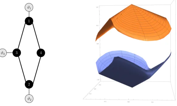
As a first example of numerical exploitation of our scheme, we investigate some properties of the Lozenge network of Figure1. With |I | = 4 and |∂I | = 3, the parameters of the model are given by
κ2 = 1 0 ε ε 0 1 ε ε ε ε 1 0 ε ε 0 1 , ε = 1 2p2, γ1= γ2= γ3= 1.
Consider first the case of thermal equilibrium: [1 : 1 : 1]. The mean heat fluxes vanish, ¯ϕ = 0. From the right pane of figure1, which shows the functionsS 3 ξ → Λ±(ξ), one infers that Condition (R) is verified so that, by Theorem3.5, the global LDP (3.11) holds with a rate function I satisfying the FR (2.20) onL⊥. 1 2 3 4 ϑ1 ϑ3 ϑ2
Figure 1: The lozenge network (left) and a plot (right) of the functions S 3 ξ 7→ Λ±(ξ) in thermal equilibrium (for the purpose of this representation, the setS has been mapped to the open unit disk).
By continuity, Condition (R) persists sufficiently near thermal equilibrium so that the same conclu-sions hold there. Figure2shows the “spectral gap”Λ+− Λ− on the boundary of the setS for dif-ferent temperature ratios. It appears that this gap eventually closes (i.e., takes non-positive values)
when the temperature differences become large. We conclude that the FR (2.20) breaks down in this regime. This is illustrated on Figure3where the rate function I and the anomalous fluctuation func-tion∆(ϕ) = I(ϕ) − I(−ϕ) − ϑ−1· ϕ are plotted for the temperature ratios [1 : 2 : 64].
Figure 2: Plot of the spectral gap∂S 3 ξ 7→ Λ+(ξ)−Λ−(ξ) of the lozenge network for different temper-ature ratios (here, the set∂S has been mapped to a circle and the polar angle 0 corresponds to the directionϑ−1).
Figure 3: The rate function I (left, the vertical line denotes the position of the average current ¯ϕ) and the anomalous fluctuation function∆ (right) for the lozenge network (see the main text for details).
4.2 A triangular network
Our second example is the triangular network already considered in [JPS] and illustrated on the left pane of Figure4. Here we have |I | = 6, |∂I | = 3 and the parameters are
κ2 = 1/2 a 0 0 0 a a 1/2 a b 0 b 0 a 1/2 a 0 0 0 b a 1/2 a b 0 0 0 a 1/2 a a b 0 b a 1/2 , a = 1 2p2, b = 1 4, γ1= γ3= γ5= 1.
In thermal equilibrium one finds thatS is the disk of radiusp3/2 centered at 0 onL⊥. The spectral gapΛ+−Λ−is open, as seen on the right pane of Figure4. Hence, here again, Theorem3.5applies: the
global LDP (3.11) and the FR (2.20) hold onL⊥near equilibrium. The spectral gap on the boundary 2 6 4 1 3 5 ϑ1 ϑ3 ϑ5
Figure 4: A triangular network (left ) and a plot (right) of the functionsS 3 ξ 7→ Λ+± (ξ) in thermal equilibrium.
Figure 5: The spectral gapΛ+− Λ−of the triangular network on the boundary∂S for different tem-perature ratios.
∂S is plotted in Figure5for various temperature ratios [ϑ1:ϑ2:ϑ3]. One observes a similar behavior as in our first example.
3 5 6 ϑ1 ϑ3 1 ϑ2 2 4 ϑ4
Figure 6: The heat pump network (left) and a plot of the functions∂S 3 ξ 7→ Λ±(ξ) for the temperature ratios [10 : 3.6 : 7 : 6.8].
Figure 7: Density plots of the spectral gapΛ+− Λ−as a function ofξ ∈ ∂S for the temperature ratios [10 : 3.6 : 7 : 6.8], [20 : 3.6 : 7 : 6.8] and [40 : 3.6 : 7 : 6.8].
4.3 A heat pump network
Our last example is the heat pump network of [EZ], see Figure6. With |I | = 6 and |∂I | = 4, the parameters: κ2 = 1 − a 0 0 0 a 0 0 1 − b 0 0 b 0 0 0 1 − a 0 0 a 0 0 0 1 − b 0 b a b 0 0 1 − 2a − b b 0 0 a b a 1 − 2a − b a = −40, b = −20, γ1= γ2= γ3= γ4= 1, ϑ1= 10, ϑ2= 3.6, ϑ3= 7, ϑ4= 6.8, were chosen in [EZ] in such a way that the mean steady heat current between the vertices 5 and 6 vanishes while the heat flows from the hot reservoir to the cold one on the left side, and from the cold to the hot one on the right side. Thus, the right side of the device acts as a heat pump. On the right
pane of Figure6we plot the two functionsΛ±on the boundary∂S .7Condition (R) is satisfied, so that the global large deviation principle (3.11) and the FR (2.20) hold onL⊥near this non-equilibrium heat pump regime.
As shown in Figure7, here again the spectral gap closes as the temperatures differences increase.
5 Proofs
5.1 Proof of Proposition3.2
In order to prove the proposition, we shall need the following two Lemmas.
Lemma 5.1. Let A and B be linear operators on a finite dimensional Hilbert space andC = V−∪ ` ∪V+
a partition of the plane into two open half-planes V±and a separating line`. Assume that (sp(A) ∪
sp(B )) ∩ ` = ; and that A and B have the same number of repeated eigenvalues in V+. Denote by A±
and B±the parts of A and B corresponding to their spectra in V±. Let K be a compact set such that (sp(A) ∪ sp(B)) ∩ V+⊂ K ⊂ V+. Then the following holds:
(1) The function f (z) = logdet¡(z − A)−1(z − B)¢ is analytic in V +\ K .
(2) For any Jordan curveγ in V+\ K “enclosing” K I γf (z) dz 2πi= − I γz f 0(z)d z 2πi= tr(A+− B+). (5.1)
Proof. (1) By assumption we can enumerate the repeated eigenvalues of A and B in such a way that sp(A) = {λ+j| j ∈ J} ∪ {λ−i | i ∈ I }, sp(B ) = {µ+j| j ∈ J } ∪ {µ−i | i ∈ I }
with
λ+
j,µ+j ∈ K ⊂ V+, λ−j,µ−j ∈ V−. In terms of these eigenvalues, we have
det¡(z − A)−1(z − B)¢ = Ã Y j ∈J z − µ+j z − λ+j ! Ã Y i ∈I z − µ−i z − λ−i ! .
The Möbius transformation z 7→z−bz−a maps the interior of the complement of any open neighborhood of the line segment joining a to b to a simply connected open subset ofC \ {0}. It follows that the function logz−bz−a is analytic on the complement of any neighborhood of the segment joining a to b. Thus, the functions z 7→ logz−µ
+ j z−λ+ j and z 7→ log z−µ− i z−λ−
i are analytic in V+\ K and so is f (z).
(2) The first identity in (5.1) now follows from integration by parts. Finally, noticing that
f0(z) =X j ∈J Ã 1 z − µ+ j − 1 z − λ+ j ! +X i ∈I Ã 1 z − µ− i − 1 z − λ− i ! = tr(z − B)−1− tr(z − A)−1, the second identity follows from the Riesz formula
− I γz f 0(z)dz 2πi= −tr µI γz(z − B) −1dz 2πi ¶ + tr µI γz(z − A) −1dz 2πi ¶ = tr(A+) − tr(B+). ä
7In Figures6and7the set∂S is mapped to the closed unit disk by first mapping ∂S to the unit sphere and then
Lemma 5.2. Let A and B be as in the previous Lemma, where` is the imaginary axis and V+the right half-plane. Then
Z +∞ −∞
log det¡(iω − A)−1(iω − B)¢dω 4π=
1
4(tr(B+− B−) − tr(A+− A−)) .
In particular, if the spectra of A and B are symmetric w.r.t.`, then tr(A−) = −tr(A+) and similarly for B ,
so
Z +∞ −∞
log det¡(iω − A)−1(iω − B)¢dω 4π = 1 2Re(tr(B+− A+)) = 1 4 X λ∈sp(B)| Re(λ)|mλ− 1 4 X λ∈sp(A)| Re(λ)|mλ ,
where mλdenotes the algebraic multiplicity of the eigenvalueλ.
Proof. Denote byγRthe positively oriented boundary of the intersection of the disk of radius R
cen-tered at 0 with the right half-plane. Applying the previous Lemma and observing that f is analytic in a neighborhood of` we get, for R large enough,
tr(A+) − tr(B+) = I γR f (z)dz 2πi= − Z R −R f (iω)dω 2π+ Z π 2 −π2 f (Reiϕ)Reiϕdϕ 2π. To evaluate the second integral on the right-hand side we note that, as R → ∞,
Reiϕ− b
Reiϕ− a= (1 − bR−1e−iϕ)(1 + aR−1e−iϕ+ O(R−2)) = 1 + (a − b)R−1e−iϕ+ O(R−2)
so logRe iϕ− a Reiϕ− b = (a − b)R −1e−iϕ + O(R−2), and
f (Reiϕ) = R−1e−i ϕtr(A − B) + O(R−2). It follows that lim R→∞ Z π 2 −π2 f (Reiϕ)Reiϕdϕ 2π = 1 2tr(A − B), and we conclude that
Z +∞ −∞ log det¡(iω − A)−1(iω − B)¢dω 4π = 1 4tr(A − B) − 1 2(tr(A+) − tr(B+)) = −1 4tr(A+) + 1 4tr(A−) + 1 4tr(B+) − 1 4tr(B−).
The last two statements follow from elementary calculations. ä
We now turn to the proof of Proposition3.2
(1) Set R(ω) = ϑ−1Q∗(A + iω)−1Q. Assumption (C) implies that A is stable (see (2.5)) so that the map R 3 ω 7→ R(ω) ∈ L(Ξ) is continuous. Using the identities
Ω = A +1 2Qϑ
−1Q∗= −A∗−1 2Qϑ
−1Q∗
a simple calculation yields that for any eξBξ ∈ Ξ one has
Eξ(ω) = Q∗(A∗− iω)−1[Ω,ξ](A + iω)e −1Q = −ζR(ω) − R(ω)∗ζ − R(ω)∗ζR(ω), (5.2) withζ = ϑ1/2ξϑ1/2. All the stated properties immediately follow.
(2) It will be convenient to introduce U (ω) = I + R(ω) and to rescale ξ by setting ζ = (ξiϑi)i ∈∂I. With
this change of variable
I − Eξ(ω) = I − Fζ(ω) = I − ζ +U(ω)∗ζU(ω),
and
D = \
ω∈R{ζ ∈ Ξ| I − Fζ(ω) > 0}, D0= {ζ ∈ Ξ | 0 < ζi< 1, i ∈ ∂I }.
It immediately follows thatD0⊂ D. Moreover, since I − Fζ(ω) is an affine function of ζ, D is convex.
Using (2.5), elementary calculations (see [JPS, Section 5.5]) show that, for anyω ∈ R, U(ω)−1= U (−ω) and |det(U (ω))| = 1. The first relation allows us to derive
I − Fζ(ω) = U(ω)∗(U (−ω)∗(I − ζ)U (−ω) − (I − ζ) + I )U (ω) = U (ω)∗(I − FI −ζ(−ω))U (ω), (5.3)
and the second one yields thatζ ∈ D ⇐⇒ I −ζ ∈ D, which shows that D is centrally symmetric around the point I /2. To show that it is open, we now argue that its complementDcis closed. Indeed,ξ ∈ Dc iff there existsω ∈ R such that Eξ(ω) has an eigenvalue λ ≥ 1. Thus, if ξnis a sequence inDcwhich
converges toξ, there exist ωn∈ R, λn≥ 1 and unit vectors unsuch that Eξn(ωn)un= λnun. Given the
fact that
1 ≤ λn≤ kEξn(ωn)k ≤ C (1 + |ωn|)
−2≤ C < ∞
one concludes that |ωn| ≤ C1/2− 1 and λn∈ [1,C ]. Thus the sequence (ξn,ωn,λn, un) has a
conver-gent subsequence with limit (ξ,ω,λ,u) satisfying Eξ(ω)u = λu, λ ≥ 1 and u 6= 0. Hence, ξ ∈ Dcand consequentlyDcis closed.
If the mapω 7→ Eη(ω) vanishes identically on R, then it follows from the identity I−Eξ+λη(ω) = I−Eξ(ω) thatD + λη ⊂ D for all λ ∈ R. Reciprocally, if the later condition holds, then for all ξ ∈ D and all λ > 0, one has
−1
λ(I − Eξ(ω)) < Eη(ω) <
1
λ(I − Eξ(ω)).
Lettingλ → ∞ we deduce that Eη(ω) vanishes identically. Note that the later condition is satisfied for anyη such that there existseηBη with Σeη= 0. This is in particular the case for η = 1 andeη = IΓ. Reciprocally, since it follows from Condition (C) that the set {(A + iω)−1Qu |ω ∈ R,u ∈ C∂I} is total in CI, one concludes that Eξ(ω) = 0 for all ω ∈ R implies Σ
e
ξ= 0 for any eξBξ.
(3) Consider first the mapD 3 η 7→ −logdet(I −Fη(ω)) for fixed ω ∈ R. The previous discussion clearly implies that it is real analytic. Its convexity follows from an elementary calculation which yields that
− X i , j ∈∂I ¯ zi ∂2 log det(I − Fη(ω)) ∂ηi∂ηj zj= tr¡(I − Fη(ω))−1/2Fz(ω)∗(I − Fη(ω))−1Fz(ω)(I − Fη(ω))−1/2¢ ≥ 0
forη ∈ D and z ∈ C∂I. From (5.2) one further deduces that Fη(ω) = O(ω−2) as |ω| → ∞, locally uni-formly inη ∈ D. It follows that
f (η) = −
Z ∞
−∞log det(I − Fη (ω))dω
4π= g (ξ) is convex and real analytic onD. The identity (5.3) leads to
det(I − Fη(ω)) = det(I − F1−η(−ω)),
and in particular det(I − F1(ω)) = 1. This proves the first equality in (3.4). The second one follows from (3.3) and the linearity of the mapη 7→ Fη.
(4) The second equality in (3.4) implies thatη · ∇g(ξ) = 0 for all ξ ∈ D and all η ∈ L . To establish the reciprocal property, note that sinceD is open, for any ξ ∈ D and any η ∈ ∇g(D)⊥there exists² > 0 such thatξ+αη ∈ D for |α| < ². It follows that the function α 7→ g(ξ+αη) is constant in a real neighborhood
of 0 and hence extends by analyticity to the constant function on the lineξ + Rη. Since, by Part (7), g is singular on∂D, it follows that ξ + Rη ⊂ D, i.e., η ∈ L .
Consequently, g vanishes identically wheneverL = Ξ. In the opposite case, the calculation in Part (3) gives that the Hessian of g satisfies
η · g00(ξ)η =Z ∞ −∞
tr³£(I − Eξ(ω))−1/2Eη(ω)(I − Eξ(ω))−1/2¤2
´dω 4π > 0
for non-zeroη 6∈ L . It follows that the restriction of g00(ξ) to L⊥is positive definite which implies that the restriction of g toS is strictly convex. To show that the closure of S is compact, let us assume thatS is unbounded. Since S is convex and centrally symmetric w.r.t. the orthogonal projection ξ0 of (2ϑ)−1ontoL⊥, it follows that for some non-vanishingξ ∈ L⊥one hasξ0+ λξ ∈ S for all λ ∈ R, i.e.,
− 1
|λ|(I − Eξ0(ω)) ≤ Eξ(ω) ≤ 1
|λ|(I − Eξ0(ω))
for allω ∈ R. Letting |λ| → ∞ yields that ξ ∈ L which contradicts the fact that 0 6= ξ ∈ L⊥.
(5) We start with some simple consequences of Condition (C). For a short introduction to the neces-sary elementary material, we refer the reader to [LR, Section 4]. Since Aξ= A +QξQ∗, the pair (Aξ,Q) is controllable for allξ. The relation A∗
ξ = −Aϑ−1−ξshows that the same is true for the pair (A∗ξ,Q).
Thus, one has
\
n≥0
Ker(Q∗Anξ) = \
n≥0
Ker(Q∗A∗nξ ) = {0}
for allξ. This implies that if Q∗u = 0 and (Aξ− z)u = 0 or (A∗ξ− z)u = 0, then u = 0, i.e., no eigenvector
of Aξor A∗ξ can live in KerQ∗. Assume now z ∈ sp(Aξ) and let u 6= 0 be a corresponding eigenvector.
Since
Aξ+ A∗ξ= 2Q(ξ − (2ϑ)−1)Q∗, taking the real part of 〈u,(Aξ− z)u〉 = 0 we infer
〈Q∗u, (ξ − (2ϑ)−1)Q∗u〉 = Re(z)|u|2.
Thus, controllability of (Aξ,Q) implies that for ±(ξ − (2ϑ)−1) > 0 one has sp(Aξ) ⊂ C±and in particular sp(Aξ) ∩ iR = ;. Hence, for ξ > (2ϑ)−1andω ∈ R, Schur’s complement formula yields
det(Kξ− iω) = | det(Aξ+ iω)|2det¡I + rξ(ω)∗ξ(ϑ−1− ξ)rξ(ω)¢ (5.4)
where we have set
rξ(ω) = Q∗(Aξ+ iω)−1Q.
One easily checks that rξ(ω) = r0(ω)(I + ξr0(ω))−1from which a simple calculation gives
I + rξ(ω)∗ξ(ϑ−1− ξ)rξ(ω) = (I + r0(ω)∗ξ)−1(I − Eξ(ω))(I + ξr0(ω))−1. Inserting the last identity into the right-hand side of (5.4) and using the fact that
det(Aξ+ iω) = det(A + iω) det(I + ξr0(ω)), we obtain
det(Kξ− iω) = | det(A + iω)|2det(I − Eξ(ω)). (5.5)
Both sides of this identity being polynomials inξ, it extends to all ξ ∈ Ξ. It follows that \
ω∈R{ξ ∈ Ξ|1 6∈ sp(Eξ(ω))} = {ξ ∈ Ξ| sp(Kξ) ∩ iR = ;}.
By continuity of the functionξ 7→ min
ω∈Rdet(I −Eξ(ω)), D is the connected component of the point ξ = 0
(6) Forξ ∈ Ξ, KξisR-linear on the real vector spaceΓ ⊕ Γ. Thus, its spectrum is symmetric w.r.t. the real axis. Observing that J Kξ+ Kξ∗J = 0, where J is the unitary operator
J =· 0 I
−I 0 ¸
,
we conclude that the spectrum of Kξ is also symmetric w.r.t. the imaginary axis. Assume now that
ξ ∈ D. Since the eigenvalues of Kξare continuous functions ofξ, Kξand K0have the same number of repeated eigenvalues in the left/right half-plane. From (5.5) we deduce
g (ξ) =
Z +∞ −∞
log det¡(iω − Kξ)−1(iω − K0) ¢ dω
4π, and Lemma5.2allows us to conclude that
g (ξ) =1 4 X λ∈sp(K0) | Re(λ)|mλ−1 4 X λ∈sp(Kξ) | Re(λ)|mλ.
Since sp(K0) = sp(A) ∪ sp(−A) and A is stable, we have X
λ∈sp(K0)
| Re(λ)|mλ= −2 X λ∈sp(A)
Re(λ)mλ= −2 Re tr(A) = tr(Qϑ−1Q∗),
and (3.6) follows forξ ∈ D. Since the eigenvalues of Kξare continuous functions ofξ ∈ Ξ, this relation extends toξ ∈ D. The boundedness of this extension follows from the translation invariance along L and the precompactness ofS .
(7) The idea of the proof is thatξ0∈ ∂D iff at least one eigenvalue of Eξ0(ω) reaches its global maximum
1 at someω0∈ R. Since Eξ0(ω) is a real analytic function of ω, the function tr¡(1 − Eξ0(ω))−1¢ has a pôle
atω = ω0, and since this function is non-negative the order of this pôle must be even. Consequently, Z ω0+²
ω0−²
tr¡(1 − Eξ0(ω))
−1¢ dω = +∞.
Forξ ∈ D, a simple calculation and Cauchy–Schwarz inequality yield |∇g (ξ)| ≥ ξ |ξ|· ∇g (ξ) = 1 |ξ| Z +∞ −∞ tr¡(I − Eξ(ω))−1Eξ(ω)¢dω 4π.
Since 0 6∈ ∂D, it suffices to show that the integral on the right-hand side diverges to +∞ as ξ → ξ0∈ ∂D. Let us fixξ0∈ ∂D and set Vδ= {ξ ∈ D | |ξ−ξ0| < δ}. Elementary considerations show that for sufficiently smallδ > 0 and sufficiently large M > 0 there exists a constant C such that
Z +∞ −∞ tr¡(I − Eξ(ω))−1Eξ(ω)¢dω 4π ≥ C µ −1 + Z M −M tr¡(I − Eξ(ω))−1¢ dω 
for anyξ ∈ Vδ. Makingδ smaller and M larger if necessary, we can assume that Jξ(ω) = (I−Eξ−ξ0(ω))−1/2 satisfies 1/p2 ≤ Jξ(ω) ≤p2 for (ω,ξ) ∈ [−M,M] ×Vδ. Writing
(I − Eξ(ω))−1= Jξ(ω)(I − Jξ(ω)Eξ0(ω)Jξ(ω))
−1J
ξ(ω)
and observing that this implies, in particular, that I − Jξ(ω)Eξ0(ω)Jξ(ω) > 0, we derive
tr¡(I − Eξ(ω))−1¢ ≥1 2tr¡(I − Jξ(ω)Eξ0(ω)Jξ(ω)) −1¢ > 0. By Fatou’s lemma lim inf D3ξ→ξ0 Z M −M tr¡(I − Eξ(ω))−1¢ dω ≥12 Z M −M tr¡(I − Eξ0(ω)) −1¢ dω
and by the above argument, the last integral is +∞.
(8) The existence and uniqueness of the maximal solutions of Eq. (2.16) as well as the stated properties of Dξfollow from [LR, Theorems 7.3.7 and 7.5.1], Part (5), and the relation Dξ= A +Q(ξQ∗−Q∗Xξ). It further follows from (3.6) and the symmetries of sp(Kξ) discussed in the proof of Part (5) that
g (ξ) =1 4tr(Qϑ −1Q∗) +1 2tr(Dξ) = 1 2tr(Dξ− D0) = − 1 2tr(Q ∗(X ξ− eξ)Q).
The proof of Proposition3.2is complete.
5.2 Proof of Proposition3.3
5.2.1 Some properties of the algebraic Riccati equations (2.16)
In order to prove Proposition3.3we shall need some properties of the algebraic Riccati equation Rξ(X ) ≡ X B X − X Aξ− A∗ξX −Cξ= 0. (5.6)
This is the purpose of the following proposition which provides a generalization of [JPS, Proposi-tion 5.5]. In the sequel, whenever we menProposi-tion a soluProposi-tion of (5.6), we always mean a self-adjoint
X ∈ L(Γ) such that Rξ(X ) = 0. We say that such a solution X is maximal (resp. minimal) if any other
solution X0∈ L(Γ) satisfies X0≤ X (resp. X0≥ X ). Proposition 5.3. Assume that Condition (C) holds.
(1) Forξ ∈ D the Riccati equation (5.6) has a unique maximal solution Xξ and a unique minimal solution −θXϑ−1−ξθ. Moreover, the matrix
Dξ= Aξ− B Xξ is stable and satisfies
Yξ= Xξ+ θXϑ−1−ξθ > 0.
(2) Ifξ0∈ ∂D is finite, then the non-tangential limit
Xξ0= lim D3ξ→ξ0
Xξ
exists and is the maximal solution of the corresponding limiting Riccati equationRξ0(X ) = 0.
(3) The functionD 3 ξ 7→ Xξ∈ L(Γ) is real analytic and concave. Moreover, Xξ< 0 for ξ < 0, Xξ> 0 for ξ in the convex hull of the setD0∪ {ξ ∈ D | ξ > ϑ−1}, X0= 0 and Xϑ−1= θM−1θ.
(4) For anyξ ∈ D and η ∈ L one has
Xξ+η= Xξ+eη. (5) For t > 0, set Mξ,t= Z t 0 esDξB esD∗ξds > 0.
Then, for allξ ∈ D one has
lim
t →∞M
−1
ξ,t= inft >0Mξ,t−1= Yξ≥ 0,
(6) Set∆ξ,t= Mξ,t−1− Yξ. For allξ ∈ D, one has et D∗ξM−1 ξ,tet Dξ= θ∆ϑ−1−ξ,tθ, (5.7) and lim t →∞ 1 tlog det(∆ξ,t) = 4g (ξ) − tr(Qϑ −1Q∗).
In particular, forξ ∈ D, ∆ξ,t→ 0 exponentially fast as t → ∞.
(7) LetDeξ= θDϑ−1−ξθ. Then
YξetDe∗ξ
= et D∗ξYξ
for allξ ∈ D and t ∈ R. (8) Forξ ∈ D and η ∈ Ξ η · ∇g(ξ) =1 2tr ³ ΣηeY −1 ξ ´
Proof. We refer to [LR] for a detailed introduction to algebraic Riccati equations (see also the Ap-pendix in [JPS] for a summary of the necessary basic facts). Our proof is similar to that of [JPS, Propo-sition 5.5]. The Hamiltonian matrix Kξassociated to the Riccati equation (5.6) is given by Eq. (3.5). LetH be the complex Hilbert space CΞ ⊕ CΞ on which Kξacts. The operator
Θ = ·
0 θ
θ 0
¸
acts unitarily onH . We have already observed in the proof of Proposition3.2(6) that forξ ∈ Ξ, the spectrum of Kξis symmetric w.r.t. the real axis and the imaginary axis. The time-reversal covariance relations
θAξθ = A∗ξ= −Aϑ−1−ξ, θBθ = B∗= B, θCξθ = Cξ∗= Cξ= Cϑ−1−ξ, (5.8)
which follow easily from the definitions of the operators Aξ, B , Cξ, further yieldΘKξ− Kϑ−1−ξΘ = 0
which implies
sp(Kξ) = sp(Kϑ−1−ξ). (5.9)
LetH−(Kξ) be the spectral subspace of Kξfor the part of its spectrum in the open left half-planeC−. (1) By Proposition3.2(5), sp(Kξ) ∩ iR = ; for ξ ∈ D and the existence and uniqueness of the maximal and minimal solutions of the Riccati equation (5.6) follow from [LR, Theorems 7.3.7 and 7.5.1]. The relation between minimal and maximal solutions is a consequence of the Relations (5.8) which imply that
Rξ(θX θ) = θRϑ−1−ξ(−X )θ.
By [LR, Theorems 7.5.1], the maximal solution Xξis related to the spectral subspaceH−(Kξ) by
H−(Kξ) = Ran · I Xξ ¸ , moreover, sp(Dξ) = sp(Kξ) ∩ C−.
Yξ= Xξ+ θXϑ−1−ξθ is called the gap of Eq. (5.6). As the difference between its maximal and minimal
solutions, it is obviously non-negative. It further has the remarkable property that for any solution X , ker(Yξ) is the spectral subspace of Aξ−B X for the part of its spectrum in iR [LR, Theorem 7.5.3]. Since sp(Dξ) ⊂ C−, we must have Yξ> 0.
(2) Letξ0∈ ∂D be finite and η 6= 0 be non-tangential to ∂D at ξ0. Setξt = ξ0− t η. W.l.o.g. we may assume thatξ1∈ D. The function
]0, 1] 3 t 7→ Zt= Xξt+ t X
0
is concave and its first derivative vanishes at t = 1. Hence, it is monotone non-decreasing. We claim that the set {Xξ| ξ ∈ D, |ξ| < r } is bounded in L(Γ) for any finite r . It thus follows that
X = lim
t ↓0Xξt= limt ↓0Zt= inft ∈]0,1]Zt
exists. By continuity, one has Rξ0(X ) = 0 and sp(Aξ0− B X ) ⊂ C−, and it follows from [LR,
Theo-rem 7.5.1] that X is the maximal solution of the limiting Riccati equation. In particular, the non-tangential limit exists (i.e., does not depend on the direction).
To prove our claim, we first derive a bound on ˆXξ= Q∗XξQ. Using (Q∗X
ξQ)2≤ kQk2Q∗Xξ2Q, one
easily deduces from (5.6) and Cauchy-Schwarz inequality
tr( ˆXξ2) ≤ kQk2tr(Q∗Xξ2Q) = kQk2¡tr(Cξ) + 2tr( ˆXξ(ξ − (2ϑ)−1))¢ ≤ bξ+ aξtr( ˆXξ2)1/2,
where aξand bξare locally bounded functions ofξ. Solving the resulting quadratic inequality yields that tr( ˆXξ2), and hence tr(Q∗Xξ2Q) are locally bounded as functions ofξ. Rewriting (5.6) as the Lya-punov equation
XξA + A∗Xξ= Fξ≡ XξB Xξ− XξQξQ∗−QξQ∗Xξ−Cξ,
and using the fact that A is stable, we get
Xξ= − Z ∞
0
et A∗Fξet Adt . It follows that for any T ∈ L(Γ)
| tr(T Xξ)| ≤ Z ∞ 0 ¯ ¯ ¯tr ³ et AT et A∗Fξ´¯¯ ¯ dt ,
from which one easily concludes that kXξk is locally bounded.
(3) The spectral projection of Kξfor the part of its spectrum inC+can be written as
Pξ= · I Xξ ¸ Yξ−1£ θXϑ−1−ξθ I ¤ = " I − Yξ−1Xξ Yξ−1 Xξ(I − Yξ−1Xξ) XξY−1 ξ # .
SinceD 3 ξ 7→ Pξ is real analytic by regular perturbation theory, Yξ−1 and XξYξ−1 are real analytic function ofξ ∈ D. The same holds for Yξand Xξ= XξYξ−1Yξ.
Invoking the implicit function theorem and using the stability of Dξ, one easily computes derivatives of the mapD 3 ξ 7→ Xξ. The first derivative is the linear map
Ξ 3 η 7→ X0 ξ[η] =eη − Z ∞ 0 et D∗ξΣ e ηet Dξdt , (5.10)
where, as usual, we identifyη ∈ Ξ with the corresponding diagonal matrix in L(Ξ) andeηBη. The second derivative is the quadratic form
Ξ 3 η 7→ X00 ξ[η] = −2 Z ∞ 0 et D∗ξ(X0 ξ[η] −eη)B(X 0 ξ[η] −eη)e t Dξdt ,
and concavity follows from the obvious fact that X00
ξ[η] ≤ 0.
To prove the inequalities let us rewrite the Riccati equation (5.6) as a Lyapunov equation
XξAξ+ A∗ξXξ= XξB Xξ−Cξ,
and recall that, as established in the proof of Proposition3.2(5), ∓Aξis stable for ±(ξ − (2ϑ)−1) > 0.
Thus, we have ∓Xξ= − Z ∞ 0 e∓t A∗ξ(XξB Xξ−Cξ)e∓t Aξdt ≤ Z ∞ 0 e∓t A∗ξCξe∓t Aξdt ,


![Figure 7: Density plots of the spectral gap Λ + − Λ − as a function of ξ ∈ ∂S for the temperature ratios [10 : 3.6 : 7 : 6.8], [20 : 3.6 : 7 : 6.8] and [40 : 3.6 : 7 : 6.8].](https://thumb-eu.123doks.com/thumbv2/123doknet/14664984.740527/17.892.119.781.580.763/figure-density-plots-spectral-gap-function-temperature-ratios.webp)
