Multidimensional Riemann Problem with Self-Similar Internal Structure – Part III– A Multidimensional Analogue of the HLLI Riemann Solver for Conservative Hyperbolic Systems

HAL Id: hal-01426759

https://hal.inria.fr/hal-01426759

Preprint submitted on 4 Jan 2017

HAL is a multi-disciplinary open access archive for the deposit and dissemination of sci-entific research documents, whether they are pub-lished or not. The documents may come from teaching and research institutions in France or abroad, or from public or private research centers.

L’archive ouverte pluridisciplinaire HAL, est destinée au dépôt et à la diffusion de documents scientifiques de niveau recherche, publiés ou non, émanant des établissements d’enseignement et de recherche français ou étrangers, des laboratoires publics ou privés.

Multidimensional Riemann Problem with Self-Similar

Internal Structure – Part III– A Multidimensional

Analogue of the HLLI Riemann Solver for Conservative

Hyperbolic Systems

Dinshaw Balsara, Boniface Nkonga

To cite this version:

Dinshaw Balsara, Boniface Nkonga. Multidimensional Riemann Problem with Self-Similar Internal Structure – Part III– A Multidimensional Analogue of the HLLI Riemann Solver for Conservative Hyperbolic Systems. 2017. �hal-01426759�

1

Multidimensional Riemann Problem with Self-Similar Internal Structure –

Part III– A Multidimensional Analogue of the HLLI Riemann Solver for

Conservative Hyperbolic Systems

By

Dinshaw S. Balsara1 and Boniface Nkonga2

1_{Physics Department, University of Notre Dame, USA (dbalsara@nd.edu)} 2_{Universiteé de Nice-Sophia Antipolis, UMR CNRS & Inria Sophia Antipolis, France}

(boniface.nkonga@unice.fr)

Abstract

Just as the quality of a one-dimensional approximate Riemann solver is improved by the inclusion of internal sub-structure, the quality of a multidimensional Riemann solver is also similarly improved. Such multidimensional Riemann problems arise when multiple states come together at the vertex of a mesh. The interaction of the resulting one-dimensional Riemann problems gives rise to a strongly-interacting state. We wish to endow this strongly-interacting state with physically-motivated sub-structure. The fastest way of endowing such sub-structure consists of making a multidimensional extension of the HLLI Riemann solver for hyperbolic conservation laws. Presenting such a multidimensional analogue of the HLLI Riemann solver with linear sub-structure for use on structured meshes is the goal of this work. The multidimensional MuSIC Riemann solver documented here is universal in the sense that it can be applied to any hyperbolic conservation law.

The multidimensional Riemann solver is made to be consistent with constraints that emerge naturally from the Galerkin projection of the self-similar states within the wave model. When the full eigenstructure in both directions is used in the present Riemann solver, it becomes a complete Riemann solver in a multidimensional sense. I.e., all the intermediate waves are represented in the multidimensional wave model. The work also presents, for the very first time, an important analysis of the dissipation characteristics of multidimensional Riemann solvers. The present Riemann solver results in the most efficient implementation of a multidimensional Riemann solver with sub-structure. Because it preserves stationary linearly degenerate waves, it might also help with well-balancing. Implementation-related details are presented in pointwise fashion for the one-dimensional HLLI Riemann solver as well as the multidimensional MuSIC Riemann solver.

Several stringent test problems drawn from hydrodynamics, MHD and relativistic MHD are presented to show that the method works very well on structured meshes. Our results demonstrate the versatility of our method. The reader is also invited to watch a video

2

introduction to multidimensional Riemann solvers on

3 I) Introduction

One-dimensional Riemann solvers are routinely used in the numerical solution of hyperbolic systems of conservation laws. The one-dimensional Riemann problem is a self-similar solution that results from a discontinuity between two constant states. In their numerical study of the multidimensional Riemann problem, Schulz-Rinne, Collins & Glaz [61] initialized four states around the center of a two-dimensional Cartesian mesh. While one-dimensional Riemann problems arise between each pair of states, those authors showed that the one-dimensional Riemann problems interact amongst themselves to form a self-similarly evolving strongly-interacting state. This strongly-interacting state arises at the point where the four states come together. The study of the multidimensional Riemann problem is, therefore, the study of the strongly-interacting state. This strongly-interacting state emerges by propagating into the one-dimensional Riemann problems along its boundary. Consequently, the strongly interacting state, as well as the one-dimensional Riemann problems that form its boundary, evolve in a self-similar fashion. We refer to this boundary as the boundary of the multidimensional wave model because it contains the strongly-interacting state. The wave models in all the multidimensional Riemann solvers incorporate this concept of self-similarity. Schulz-Rinne, Collins & Glaz [61] only presented a computational study of the multidimensional Riemann problem. However, Abgrall [1], [2] was the first to formulate multidimensional Riemann solvers that were usable. The self-similarly evolving strongly-interacting state is an inevitable consequence of having a multidimensional wave model that propagates into the one-dimensional Riemann problems. Seizing on this insight, Balsara [15] presented a self-similar formulation of the multidimensional Riemann problem. Incorporating the physics of the strongly-interacting state has shown to be very advantageous in second order calculations (Balsara [4]) and higher order accurate calculations (Balsara [15]). This is the true motivation for our study of the multidimensional Riemann solver reported here.

Following Abgrall [1], [2], further advances were also reported (Fey [40], [41], Gilquin, Laurens & Rosier [44], Brio, Zakharian & Webb [26]). However, these early formulations were cumbersome and did not see much use. Multidimensional Riemann solvers that are very efficient have also been designed and we focus on a certain class of multidimensional Riemann solvers here (Wendroff [70], Balsara [3], [4], [15], [18], Balsara, Dumbser & Abgrall [14], Vides, Nkonga & Audit[70], Balsara & Dumbser [16], Balsara et al. [19]). A video introduction to multidimensional Riemann solvers is available on the following website:

http://www.nd.edu/~dbalsara/Numerical-PDE-Course . Such Riemann solvers are applied at the

vertices of a two-dimensional or three-dimensional mesh. Many states come together at a vertex from different directions, making it possible to communicate the multidimensionality of the flow to the multidimensional Riemann solver. At the vertex, the job of the multidimensional Riemann solver is to approximate the self-similar multidimensional structure that emanates from the vertex.

4

By this point in time, there has been substantial progress in one-dimensional and multidimensional Riemann solvers. In this paragraph we list the one-dimensional Riemann solvers and juxtapose them with their multidimensional counterparts. Such a juxtaposition can be very useful in building perspective. Several excellent one-dimensional Riemann solvers have been designed. There are exact Riemann solvers from Godunov [45],[46] and van Leer [68] and two-shock approximations thereof (Colella [32], Colella & Woodward [33]). See also the work of Chorin [30]. The linearized Riemann solver by Roe [59] has also proved useful. The multidimensional Riemann solver by Abgrall [1], [2] can be viewed as Roe-type Riemann solver that has been extended to multiple dimensions. One-dimensional HLL Riemann solvers (Harten, Lax & van Leer [48]) have now been extended to two-dimensions (Balsara [3], [4]) and three-dimensions (Balsara [18]). The papers by Balsara offer simple closed form expressions for the multidimensional HLL fluxes that are easy to implement. One-dimensional HLLC Riemann solvers (Toro, Spruce and Speares [65] [66], [67], Chakraborty & Toro [29] and Batten et al. [24]) seek to restore the physics of the contact discontinuity. Multidimensional extensions of the HLLC Riemann solver to structured and unstructured meshes have also become available in recent papers (Balsara [4], Balsara, Dumbser & Abgrall [14]). While HLLC Riemann solvers seek to restore an isolated contact discontinuity in the HLL Riemann solver, it is always interesting to ask if there are other ways to introduce an intermediate wave into the HLL Riemann solver? The one-dimensional HLLE/HLLEM Riemann solver (Einfeldt [38], Einfeldt et

al. [39]) tried to do that by introducing a linear profile in the Riemann fan. However, because of

an error in the formulation, it did not achieve its intended goal. Dumbser & Balsara [37] rectified the prior deficiencies and also introduced another very important advance. Using the self-similar formulation of Balsara [15], they were able to introduce multiple intermediate waves into the HLL Riemann solver, thus giving rise to the HLLI Riemann solver. Here “I” stands for intermediate waves and acknowledges the fact that the HLLI Riemann solver can accommodate any intermediate wave as long as its eigenstructure is known. The result is a one-dimensional HLLI Riemann solver that benefits from all the good properties of the one-dimensional HLL Riemann solver and simultaneously functions as a Riemann solver that retains sub-structure. When all the intermediate waves are included, the one-dimensional HLLI Riemann solver of Dumbser & Balsara [37] becomes a complete Riemann solver. It is also a fully capable replacement for costlier Riemann solvers by Osher and Solomon [58] and Dumbser and Toro [36]. It is, therefore, very attractive to present a two-dimensional analogue of the HLLI Riemann solver for hyperbolic conservation laws and that is indeed the first goal of this paper. Such a multidimensional Riemann solver can be made complete in a multidimensional sense if all the intermediate waves in all directions are included. This is a very attractive property and we explore it further in this paper.

Self-similarity has not been used much in the design of one-dimensional Riemann solvers; the only real exception being the HLLI Riemann solver of Dumbser & Balsara [37]. However, it is crucially important in the development of multidimensional Riemann solvers (Balsara [15], Balsara & Dumbser [16]). This has prompted the name of MuSIC Riemann

5

solvers, where MuSIC stands for “Multidimensional, Self-similar, strongly-Interacting, Consistent”. Such Riemann solvers are multidimensional; they draw on the self-similarity of the problem; they focus on the strongly-interacting state that results when multiple one-dimensional Riemann solvers interact; and the design relies on establishing consistency with the conservation law. MuSIC Riemann solvers that rely on a Petrov-Galerkin projection to obtain the self-similar variation in the strongly interacting state have been presented (Balsara [15], Balsara & Dumbser [16]). An alternative projection method consists of satisfying the one-dimensional shock jumps at the boundary of the multidimensional wave model. Vides, Nkonga & Audit[70] and Balsara et

al. [19] developed a multidimensional Riemann solver without and with sub-structure

respectively that uses least squares minimization methods. A study of the dissipation characteristics of MuSIC Riemann solvers has never been presented. The second goal of this paper is to present a thorough study of the dissipation characteristics of the MuSIC Riemann solvers. We first present an analysis of the dissipation characteristics of the one-dimensional HLLI Riemann solver. We then show that when the one-dimensional HLLI Riemann solver is used as a building block for the MuSIC Riemann solver, its dissipation characteristics mirror those of the HLLI Riemann solver for flows that are mesh-aligned.

It is also worth recalling that the one-dimensional HLLI Riemann solver of Dumbser & Balsara [37] is a universal Riemann solver; i.e. it is applicable to any hyperbolic conservation law. It would be very desirable to have a multidimensional Riemann solver that is also applicable to any conservation law. The third goal of this paper is to show that when the one-dimensional HLLI Riemann solver is used as a building block for the MuSIC Riemann solver we indeed get a universal multidimensional Riemann solver that works for any hyperbolic conservation law. This generality implies that multidimensional Riemann solvers with sub-structure can be built and incorporated into any code for any hyperbolic conservation law. Moreover, the same coding strategy can be used for all hyperbolic conservation laws.

Magnetohydrodynamics (MHD) is an interesting example of a hyperbolic system with a more complex wave foliation. One-dimensional linearized Riemann solvers for numerical MHD have been designed (Roe & Balsara [60], Cargo and Gallice [27], Balsara [5]). HLLC Riemann solvers, capable of capturing mesh-aligned contact discontinuities, have been presented by Gurski [47] and Li [53]. Miyoshi and Kusano [56] drew on Gurski’s work to design an HLLD Riemann solver for MHD. It is, therefore, interesting to show that MHD can also be accommodated within our formulation. MHD is a system with an involution constraint, where the divergence of the magnetic field is always zero. Balsara & Spicer [6] showed that this is assured within the context of a higher order Godunov scheme by using the upwinded fluxes at the edges of the mesh to update the magnetic fields that are collocated at the faces of a mesh. Gardiner & Stone [42], [43] have claimed that the dissipation in those upwinded fluxes needs to be doubled all the time in order to stabilize the method. A substantial body of work now exists to show that the suggestion of Gardiner & Stone is completely unnecessary when multidimensional Riemann solvers are used to provide a properly upwinded electric field at the edges of the mesh

6

(Balsara [4], Vides, Nkonga & Audit[69], Balsara & Dumbser [17]). Indiscriminate doubling of the dissipation, as per Gardiner & Stone’s suggestion, can indeed lead to excessive dissipation of the magnetic field in the direction that is transverse to the upwind direction. The present paper reinforces that finding.

As with classical MHD, progress has also been made in relativistic MHD (RMHD). Balsara [22] and Komissarov [52] have designed Roe-type Riemann solvers for RMHD. HLLC and HLLD type Riemann solvers for RMHD have also been designed by Mignone & Bodo [54], Honkkila & Janhunen [49], Mignone, Ugliano and Bodo [55] and Kim & Balsara [51]. Balsara and Kim [20] have also shown the value of multidimensional Riemann solvers for RMHD calculations. The present paper reinforces the utility of MuSIC Riemann solvers for accurate RMHD simulations.

Section II describes a one-dimensional HLLI Riemann solver for conservation laws that is indeed novel and has some rather nice properties. Section III provides details associated with the construction of the multidimensional Riemann problem on Cartesian meshes. Section IV shows that schemes that use the multidimensional Riemann solver meet their design accuracy. Section V shows the results of several stringent test problems drawn from Euler, MHD and relativistic MHD flow. Section VI presents conclusions.

II) Quick Derivation of the One-Dimensional HLLI Riemann Solver

In any multidimensional Riemann problem, the strongly-interacting state propagates into a sequence of one-dimensional Riemann problems that lie on its boundary. One dimensional Riemann solvers are, therefore, used as building blocks for the multidimensional Riemann problem. Because we wish to show that the dissipation characteristics of the MuSIC Riemann solver strongly mirror those of the one-dimensional HLLI Riemann solver, we first present a quick derivation of the one-dimensional HLLI Riemann solver in Sub-section II.a and study its dissipation characteristics in Sub-section II.b. This study is somewhat different from the one presented in Dumbser & Balsara [37] because the prior work did not use one of the Galerkin constraints that results from the imposition of self-similarity. A compare-and-contrast is presented in Sub-section II.c. Sub-section II.d presents implementation-related details. In Section III we present a multidimensional Riemann solver in two-dimensions that is a close analogue of the one-dimensional HLLI Riemann solver presented here when Cartesian meshes are used.

II.a) Galerkin Formulation in Similarity Variables

In this section we consider an N-component hyperbolic conservation law,

0

t x

∂ ∂ + ∂ ∂ =U F , which is restricted to one dimension. For this conservation law, consider the Riemann fan between two states, U_L to the left and U_Rto the right. The Riemann problem evolves self-similarly with bounding speeds, S to the left and _L S to the right. Consider _R

7

(

)

(

)

with 2 ; c c SR SL SR SL ξ ξ ξ ξ ξ ξ  −  ≡_{ } ≡ + ∆ ≡ − ∆    (2.1)

Since the solution evolves self-similarly within the Riemann fan, the solution within the Riemann fan can be written in terms of similarity variables. Written in these shifted similarity variables, the conservation law becomes

(

)

1 0 c ξ ξ ξ ξ ξ   ∂_ − + ∆ _{ + =} ∆ ∂ F U U    (2.2)

The tilde on the top of U is intended to signify a self-similarly evolving solution. The same is true for F . Because of self-similarity, U and F are functions of only one similarity variable ξ . Eqn. (2.2) is then the governing equation written in terms of the similarity variable. We expand our state and flux as

( )

ξ = + ξξ U U U (2.3) and

( )

( ) with ξ ξ = + ξ =∂ ∂ F U F F A U A U  (2.4)

Please note that we have evaluated the characteristic matrix A by using the mean state U ; but there is some flexibility in the evaluation of the characteristic matrix. For example, it can be evaluated using Roe-averages or arithmetic averages, as was done in Dumbser and Balsara [37]. Please also note that U_ξ ≠ ∆ ∆U ξ where ∆ ≡U

(

U_R −U_L

)

. Realize that ∆ ∆U

ξ

is indeed an estimate of the full gradient and, therefore, includes contributions from the extremal waves that make up the Riemann fan. In a numerical Riemann problem, we only want to pick out contributions from waves that are internal to the Riemann fan. We will soon show that U will _ξ

be obtained by a projection of ∆U onto the subset of waves that are interior to the Riemann fan. Multiplying the conservation law from eqn. (2.2) with the test function φ ξ

( )

gives

( )

(

)

{

}

₍

₎

( )

_{( )}

1 1 0 c c φ ξ ξ ξ ξ _{φ ξ} ξ ξ ξ φ ξ ξ ξ ξ ξ   ∂ _ − + ∆ _{ ∂}   − _ − + ∆ _ + = ∆ ∂ ∆ ∂ F U F U U      (2.5)

Now we are ready to make Galerkin projections with different test functions.

Using φ ξ

( )

= and integrating over 1 ξ∈ −

[

1/ 2,1/ 2

]

gives the usual HLL state

(

)

(

)

1 1 HLL ξ R SR R ξ L SL L = = − − + − ∆ ∆ U U F U F U (2.6)

8

In practice, one always evaluates U_HLLat the start of the calculation because it plays an important role in the rest of the calculation. This could include the construction of the characteristic matrix

A . Realize, therefore, that U_HLL from the equation above will always be a positivity-preserving state. Using φ ξ

( )

= and making a Galerkin projection gives ξ

(

)

(

)

1 1 1 1 6 2 2 6 c HLL R SR R L SL L HLL ξ ξ ξ ξ ξ ξ ξ ξ ∆ − = − − − − − ⇔ = + ∆ ∆ ∆ ∆ U F U F U F U F F U (2.7)

Here F_HLL is the classical HLL flux. With U_ξ =0 we indeed retrieve the HLL flux from the above equation, which is a good thing. But the above equation also shows that the choice of U _ξ

and F are indeed related. If we set one, we have to reset the other. In other words, endowing sub-structure to the Riemann problem by setting U_ξ ≠0 will, in general, cause a shift in the mean flux F so that it becomes different from F_HLL.

Let

{

r i_i: =1,...,N

}

and

{

l i_i: =1,...,N

}

be the full set of eigenvectors with eigenvalues

{

λ_i:i=1,...,N

}

. In other words, the previous sentence just catalogues the eigenvectors and eigenvalues of the characteristic matrix A which we have documented above. Let I_int be the set of intermediate waves that we want to represent in the Riemann fan. (We could, of course, choose I_int =N in which case all the waves in the hyperbolic system are considered. Consequently, the Riemann solver becomes a complete Riemann solver.) The best characteristic projection we can do gives us

(

)

( ) (

)

int 2 _{i i R L i} 2 _{R L} i I l r ξ δ ∈ =

∑

_ − _ = − U  U U R δ L U U (2.8)

Here R is a matrix of right eigenvectors with dimension N×

(

#I_int

)

and contains only the right eigenvectors being considered; L is a corresponding matrix of left eigenvectors with dimension

(

# Iint

)

× and N δ is a diagonal matrix of dimension

(

#Iint

) (

× #Iint

)

. Here “

(

# Iint

)

” denotes the

number of elements in the set “I_int”. We will specify the diagonal elements of δ shortly and we will see that each diagonal term

δ

_i in the diagonal matrix δ depend on the structure of the wave model as well as the wave speed

λ

_i. Therefore, in order to be consistent with the Galerkin projection, we should substitute the value of U from eqn. (2.8) in eqn. (2.7) to get the flux F . _ξ

Also please notice that when the state is endowed with sub-structure F , which is obtained from eqn. (2.7), is not the classical HLL flux. The final numerical flux at the zone boundary, i.e. at

0 ξ= , is given by

(

)

c numerical c ξ ξ ξ ξ ξ ξ = = − ∆ = − ∆ F F F A U (2.9a)

9 or

(

)

(

)

int int = 2 2 6 c c numerical i i R L i i HLL i i R L i i i I i I l r _ξ l r ξ _{δ λ} ξ ξ _{δ λ} ξ ∈ ξ ∈   _{∆  }      − _{ } − _ _= + + −_{ } _ − _{ } ∆ _

∑

_{ } ∆ _

∑

_ F F  U U F U  U U (2.9b) or

( )

2

( )

(

)

1 = 2 2 2 3 c numerical HLL R L ξ ξ ξ  ∆  − _− + _ − ∆   F F R δ Λ δ L U U (2.9c)

To clarify further, F in eqn. (2.9b) is not the HLL flux. The square bracket term in eqn. (2.9c) clearly shows that the final numerical flux is made up of an HLL flux plus an anti-diffusive contribution from the HLLI Riemann solver. Notice that the final numerical flux in eqn. (2.9c) only requires us to know the intermediate eigenvectors and eigenvalues that we want to represent in our wave model. Therefore, the original advantage of the HLLI Riemann solver is preserved. What is new here is the incorporation of the Galerkin constraint stemming from eqn. (2.7).

Let us now obtain

δ

_i by paying careful attention to the numerical viscosity of the proposed HLLI Riemann solver. Using expressions from Appendix B of Dumbser & Balsara [37] we write the last line of eqn. (2.9) as

(

)

(

)

(

)

(

)

(

) ( ) (

(

)

) ( )

(

)

1 2 2 1 2 2 2 3 numerical R L R L R L R L R L R L R L R L R L S S S S S S S S S S S S S S = +  + − +  − _ − − + _ − − − −   F F F R Λ I δ Λ δ L U U (2.10) The second term in the above equation helps us to identify the viscosity of our Riemann solver. The square bracket in the above equation gives us the eigenvalues of the viscosity matrix and we want these to be bounded by the eigenvalues of the Roe-matrix viscosity (at the lower end) and the eigenvalues of the HLL viscosity (at the upper end). Using the dissipation properties of the underlying HLL Riemann solver we get the condition for

δ

_i as follows

(

)

(

)

(

)

(

)

(

)

2 2 2 when 3 0 min , otherwise 3 3 where = i R L i R L i R i L i R L i R L i R L R L i R L S S S S S S S S S S S S S S S S φ λ δ _{λ λ} φ λ φ − +   _{− − +} _≤     _{ } =  _{ + − }  _{ }    _ − − + _ _  − − (2.11)

10

This condition ensures that our dissipation minimally matches or exceeds the dissipation of the Roe matrix for the sake of stability. Here λ_i− ≡min

(

λ_i, 0

)

and λ_i+ ≡max

(

λ_i, 0

)

. In fact, the choice of

φ

_i in eqn. (2.11) is not mandated by mathematics but rather by our desire to capture stationary linearly degenerate waves, like contact discontinuities, exactly on the mesh. In other words, when _

(

S_R−S_L

)

2 3−λ_i

(

S_R +S_L

)

_≤0 we have the option to set

φ

_i to a value that may even be greater than half. To capture stationary contact discontinuities exactly, we set

φ

_i in such a way that the dissipation terms in the square bracket in eqn. (2.10) tend to zero as

λ

_i →0 . Notice too that

φ

_i is always positive for the sub-sonic case so that the gradient that is provided in eqn. (2.8) is always physical. In the subsonic case, i.e. when SL< <0 SR, the maximum positive value that can be assumed by

φ

_i is 3 4 which occurs when S_R = −S_L. Entropy is naturally enforced in this Riemann solver because the Riemann fan automatically provides a linear variation in the sub-structure.

Notice that when “I_int” is a complete set of intermediate waves, i.e. when I_int =N, the one-dimensional HLLI Riemann solver is indeed complete. Positivity is also very easily addressed in the context of this formulation. Notice that eqns. (2.8) and (2.11), along with the eigenstructure of the intermediate waves, fully specify U . One has only to ensure that _ξ U

( )

ξ

with our present choice of sub-structure remains positive for ξ∈ −

[

1/ 2,1/ 2

]

. In practice, this positivity-enforcement is best done by checking for positivity at the ends of the interval; i.e., for the states U_HLL+U_ξ 2 and U_HLL−U_ξ 2 . If positivity is not met, one is free to reduce U . In _ξ

the limit of U_ξ =0, the present Riemann solver reduces exactly to an HLL Riemann solver thereby guaranteeing positivity; see eqn. (2.9c).

Also notice that when S_R  S_L or when S_L  S_R , we have

δ

_i →0 so that

numerical → HLL

F F . Now recall the very nice design feature of the HLL Riemann solver which says that the subsonic flux retrieves the supersonic fluxes when the Riemann fan is opened up ever so slightly so as to always force it to be minimally subsonic. From the property stated at the beginning of this paragraph we see that our HLLI Riemann solver also retains that very nice design feature.

II.b) Dissipation Properties of the present HLLI Riemann solver

Recall that the Roe-type Riemann solver provides the theoretical minimum dissipation that any Riemann solver should provide to a scheme in order to ensure stability of the numerical method. However, the Roe-type Riemann solver has problems with positivity enforcement, while the HLLI Riemann solver discussed in this Section is free of this problem. The entropy fix is also naturally built into the HLLI Riemann solver. It is, therefore, worth asking the question, “How much excess dissipation is produced by the present HLLI Riemann solver compared to the Roe-type Riemann solver?”. We answer that question in this paragraph and the next one. To normalize the search space, we can always require S_R−S_L = . We also require 1 S_L ≤ ≤0 S_R, i.e.

11

we focus on the subsonic case. We assume that there is only one intermediate wave with wave speed λ such that _i S_L ≤λ_i ≤S_R. (Since the dissipation is independently determined for each wave family, the number of wave families that we use does not affect our present analysis.) For such a wave, we can use eqn. (2.11) to evaluate δ . The square bracket in eqn. (2.10) then gives _i us the dissipation matrix. The diagonal term in the dissipation matrix for the intermediate wave being considered should be greater than or equal to λ_i because this is the theoretically minimum amount of dissipation required by the Roe-type Riemann solver. For various subsonic choices of S and _L S , and with the normalizing restriction _R S_R−S_L = , we can indeed step 1 through all possible values of λ . We can then plot the dissipation produced by the present _i HLLI-style Riemann solver versus λ . We can also plot _i λ_i , the dissipation from the Roe-type Riemann solver, versus λ . Such an exercise is undertaken in the next paragraph and it enables i

us to get an interesting perspective on the dissipation characteristics of the present HLLI Riemann solver vis a vis the Roe-type Riemann solver.

The previous paragraph outlined a strategy for quantifying the dissipation properties of the HLLI Riemann solver and comparing it to the Roe-type Riemann solver. The results of this exercise are shown in Fig. 1. The dashed lines in Fig. 1 show the dissipation from our HLLI Riemann solver whereas the solid lines show the dissipation from the Roe-type Riemann solver. Fig. 1a shows us the dissipation from the HLLI Riemann solver and also the theoretically minimum dissipation, λ_i , on the vertical axis as a function of wave speed, λ , on the horizontal _i axis when S_L = −0.9 and S_R =0.1. We see from Fig. 1a that our HLLI-style Riemann solver always produces dissipation that is within 23.2% of the Roe-type Riemann solver. (Please also note that the analogous plot for SL = −0.1 and SR =0.9 would look identical to Fig. 1a after it is

flipped about the vertical axis given by λ = . This trend extends to all the other panels in Fig. i 0 1.) Fig. 1b shows similar information when SL = −0.7 and SR =0.3. From Fig. 1b we see that

the dissipation of the HLLI-style Riemann solver coincides with the dissipation of the Roe-type Riemann solver when S_L = −0.7 and S_R =0.3. Fig. 1c shows similar information when

0.5

L

S = − and S_R =0.5; again showing us that the two Riemann solvers produce identical dissipation. Fig. 1d shows similar information when S_L = −0.2 and S_R =0.8; again showing us that our HLLI Riemann solver always produces dissipation that is within 17.6% of the Roe-type Riemann solver. Fig. 1e shows analogous information when S_L = −0.01 and S_R =0.99; we see that the dissipation of the two Riemann solvers is almost identical. Based on such an analysis, we conclude that our present HLLI Riemann solver always produces dissipation that is within ten to twenty percent of the Roe-type Riemann solver under all circumstances. In many of the situations shown in Fig. 1, the two Riemann solvers have identical dissipation. This is a very interesting demonstration in light of the versatility, robustness and favorable positivity properties of our HLLI Riemann solver and the lack thereof for the Roe-type Riemann solver. For all the panels in Fig. 1 we see that our HLLI Riemann solver has zero dissipation when λ_i = which 0 shows that it can also capture stationary linearly degenerate waves exactly. Consequently, we see that it offers all the good attributes of the Roe-type Riemann solver while avoiding all its pitfalls. Fig. 1 of this paper can also be compared to Fig. 3.1 of Castro-Díaz and Fernández-Nieto [28] if

12

one wants to analyze the dissipation properties of the HLLI Riemann solver through the perspective of polynomial viscosity methods (PVM).

II.c) Comparison with the HLLI-type Riemann solver of Dumbser and Balsara [37]

In this section we have designed an HLLI-type Riemann solver based on endowing sub-structure to the HLL Riemann solver. The one-dimensional HLLI Riemann solver described here is very useful because it extends more naturally to multidimensions. In Dumbser and Balsara [37] a slightly different HLLI-type Riemann solver had been presented. The difference is primarily in the fact that the Galerkin projection in eqn. (2.7) is not used in the design of the Riemann solver in Dumbser & Balsara [37]. As a result, eqns. (2.9) and (2.11) are also substantially different. It is interesting to compare and contrast the two variants of HLLI Riemann solvers. To that end, it is valuable to write the explicit expressions for U 

( )

ξ and F 

( )

ξ

for the present HLLI Riemann solver for any value of the similarity variable ξ=x t . The formulae in this paragraph are valid as long as ξ lies in the range S_L< <ξ S_R, i.e. within the Riemann fan. Using δ from eqn. (2.11), we get _i

( )

(

)

( )

(

)

(

)

int int int 2 2 2 6 c HLL i i R L i i I c HLL i i R L i i i R L i i i I i I l r l r l r ξ ξ ξ δ ξ ξ ξ ξ ξ δ δ λ ξ ∈ ∈ ∈    −   = +_{ } _ − _{ } ∆ _{ }        −   ∆     = + _{ } − _{ }+_{ } _ − _{ } ∆         

∑

∑

∑

U U U U F F U U U U    _    _{ } (2.12)

The two curly brackets in the above two equations only need to be evaluated once. Appendix A provides the corresponding formulation of this Riemann solver for moving meshes, i.e., ALE-type meshes. Notice that the Galerkin formulation from eqn. (2.7) dictates that the inclusion of sub-structure should cause a change in the mean flux in eqn. (2.12). It is also helpful to be able to compare and contrast this Riemann solver with the HLLI Riemann solver from Dumbser and Balsara [37]. That Riemann solver does not use the first moment of the conservation law, i.e. eqn. (2.7), because it is meant to be generally applicable to hyperbolic systems in conservation and non-conservative forms. As a result, the definition of δ changes to _i

1 i i i L R S S λ λ δ = − − − + (2.13)

For the Riemann solver from Dumbser and Balsara [37] we then have

( )

(

)

( )

(

)

int int 2 2 2 2 c HLL i i R L i i I R L HLL i i R L i i I l r S S l r ξ ξ ξ δ ξ ξ ξ δ ξ ∈ ∈    −   = +_{ } _ − _{ } ∆ _{ }        −   = +_{ } _ − _{ } ∆ _{ }    

∑

∑

U U U U F F U U    _    _ (2.14)

13

Only one curly bracket needs to be evaluated in the above equation, therefore, the HLLI Riemann solver from Dumbser and Balsara [37] has slightly lower computational complexity. However, both flavors of HLLI Riemann solvers require the evaluation of the intermediate eigenvectors. This eigenvector evaluation often constitutes the bulk of the additional computational cost that is added on top of the cost of the HLL Riemann solver. For that reason, both flavors of HLLI Riemann solver have almost the same overall computational complexity. Notice that δ can assume larger values in eqn. (2.13) compared to eqn. (2.11). However, the _i mean HLL flux in eqn. (2.14) is left unchanged by the inclusion of sub-structure in the Riemann fan. The flux in eqn. (2.14) is based on considering fluctuations. Comparing the fluxes in eqns. (2.12) and (2.14) we see that the flux in the former equation varies linearly with ξ whereas the flux in the latter equation varies quadratically with ξ . This is a consequence of the different philosophies that were used in deriving the two variants of the HLLI Riemann solver. In practice, both work equally well. Both can preserve stationary intermediate waves on a mesh without additional dissipation.

II.d) Implementation-Related Details for one-dimensional HLLI Riemann solver:-

The present HLLI Riemann solver can be easily retrofitted to any HLL Riemann solver and usually provides a very palpable improvement in the simulation quality. The steps in the implementation of this one-dimensional HLLI Riemann solver are as follows:

1) Obtain U_HLL from eqn. (2.6). (If the density in U_HLL is substantially lower than the minimum density in the states U_L and U_Rwe do not provide linear sub-structure. Similarly, if the density in U_HLL is substantially greater than the maximum density in the states U_L and U_Rwe also do not provide linear sub-structure. Similar considerations are made for the pressure. I.e., this is just a reasonable and physical criterion for deciding whether it is justified to include sub-structure in the Riemann solver.)

2) Using U_HLL, obtain the eigensystem given by

{

λ_i:i∈I_int

}

,

{

r i_i: ∈I_int

}

and

{

l i_i: ∈I_int

}

. Note that only the intermediate waves of interest are needed; and these waves are usually easier to evaluate than the entire eigenstructure.

3) Using

δ

_i from eqn. (2.11), now obtain U from eqn. (2.8). _ξ

4) Check U_HLL +U_ξ 2 and U_HLL −U_ξ 2 for positivity. Reduce U as needed to enforce _ξ

positivity.

5) Using U_HLL and U in eqn. (2.7), obtain F from eqn. (2.7). _ξ

6) Now obtain the numerical flux F_numerical from eqn. (2.9a) or (2.9b). Alternatively, we can build

HLL

F in the usual way and use it to build the numerical flux Fnumerical using eqns. (2.9b) or (2.9c). 7) The supersonic cases are obvious.

14

In this section we have provided details for the one-dimensional HLLI Riemann solver on a fixed mesh. But we also realize that some people might want to apply this Riemann solver to an arbitrary Lagrangian-Eulerian (ALE) mesh. Appendix A gives the formulation of the present one-dimensional HLLI Riemann solver on a moving mesh.

III) MuSIC Riemann Solver that is closest to an HLLI Formulation – Focus on Cartesian Meshes

Sub-section III.a presents the formulation of the MuSIC Riemann solver, including a description of the inclusion of sub-structure. Section III.b presents implementation-related details.

III.a) Formulation of the MuSIC Riemann Solver

Consider the N-component hyperbolic conservation law in two-dimensions, given by

0

t x y

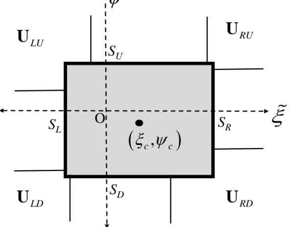
∂ ∂ + ∂ ∂ + ∂ ∂ =U F G . It can give rise to one-dimensional Riemann problems, but it can also give rise to a multidimensional Riemann problem. The multidimensional Riemann problem is most easily understood on a Cartesian mesh, and we focus on that in this paper because it is possible to get exact answers for the multidimensional Riemann solver in Cartesian geometry. We will defer the inclusion of sub-structure in the multidimensional Riemann solver on unstructured meshes for a subsequent paper. As shown schematically in Fig. 2 a multidimensional Riemann problem arises when four states U_RU , U_LU , U_LD and U_RD come together at a zone vertex; the vertex is shown as a gray dot in that figure. The four pairs of mutually contiguous states set up four dimensional Riemann problems. However, the one-dimensional Riemann problems interact in a strongly-interacting state, as shown in Fig. 2a of Balsara [15]. The strongly interacting state is bounded by a multidimensional wave model. In fig. 2a the thick solid line denotes the boundary of the multidimensional wave model; the interior of the wave model is shaded. The four initial states that come together at a vertex “O” of the mesh are also shown. The thin solid lines in Fig. 2a show the extremal speeds of the one-dimensional Riemann problems in the boundary of the multidimensional wave model. The dashed lines in Fig. 2a show the coordinate axes, measured as speeds. The bounding speeds of the multidimensional wave model are also shown. On such a mesh, the extent of the multidimensional wave model,

[

S S_L, _R

] [

× S_D,S_U

]

, is approximated beforehand. See Balsara [3] and [4] for advice on how to pick out the extent of the multidimensional wave model on a Cartesian mesh. The strongly-interacting state is bounded by the multidimensional wave model and evolves self-similarly, just like the one-dimensional Riemann problems at its boundary.

We want to predict the self-similar evolution of the multidimensional, strongly-interacting state, U . The tilde on the top of U is intended to signify a self-similarly evolving solution. Let us, therefore, pick similarity variables in two-dimensions and express the strongly-interacting state in terms of those two variables. The similarity variables are

15 ; =

x y

t t

ξ= ψ (3.1)

Notice that

( )

ξ ψ  correspond most naturally to ,

( )

x y . We make a scaled and shifted coordinate , transformation in the similarity variables with

(

)

2 ;

(

)

;

(

)

2 ;

(

)

; c R L R L c U D U D c c S S S S S S S S ξ ξ ψ ψ ξ ξ ψ ψ ξ ψ ξ ψ ≡ + ∆ ≡ − ≡ + ∆ ≡ −  −   −  ≡_{ } ≡_{ } ∆ _ ∆ _    _ (3.2)

Observe that ξ and ψ are still self-similar variables with the main difference that they now range over

[

−1/ 2,1/ 2

] [

× −1/ 2,1/ 2

]

. This makes it easier to achieve concordance with the one-dimensional case described in the previous sub-section. With the change of variables in eqn. (3.2), the N-component conservation law in two-dimensions becomes

(

)

(

)

1 1 2 0 c c ψ ψ ψ ξ ξ ξ ξ ξ ψ ψ     ∂ − + ∆ ∂_ − + ∆ _{  } + + = ∆ ∂ ∆ ∂ G U F U U      (3.3)

Here the strongly-interacting state U =U

(

ξ ψ,

)

is a function of the two similarity variables. The same is true for the fluxes F and G .

We can now expand the strongly-interacting state in the similarity variables as

(

ξ ψ,

)

= + _ξξ+ _ψψ

U U U U (3.4)

Because

(

ξ ψ,

) ( )

= 0, 0 corresponds to the centroid of our wave model, U is indeed the mean

value associated with our wave model. The x-flux is written in similarity variables as

(

)

(

)

( ) , _{ξ ψ} with ξ ψ = + ξ+ ψ =∂ ∂ F U F F A U U A U  (3.5)

It may also prove convenient to integrate eqn. (3.5) in the ψ -direction to write the numerical x-flux as

(

)

1/ 2 1/ 2 , c numerical c d ξ ξ ξ ξ ξ ψ ψ ξ −   = = − ∆ _{= −  } ∆  

∫

F F F A U (3.6)

16

(

)

(

)

( ) , _{ξ ψ} with = ξ ψ = + ξ+ ψ ∂ ∂ G U G G B U U B U  (3.7)

It also proves convenient to integrate eqn. (3.7) in the ξ -direction to write the numerical y-flux as

(

)

1/ 2 1/ 2 , c numerical c d ψ ψ ξ ψ ψ ψ ξ ψ −   = = − ∆ _{= −  } ∆  

∫

G G G B U (3.8)

For eqns. (3.6) and (3.8) recall that the time axis corresponds to

( )

ξ ψ = ,

( )

0, 0 (or alternatively,

(

ξ ψ,

) (

= −ξ_c ∆ −ξ ψ, _c ∆ψ

)

). We want to make sure that eqns. (3.6) and (3.8) meet two important goals. First, for problems with strong discontinuities in arbitrary directions the expressions for F_numerical and G_numerical generate sufficient entropy to stabilize the problem. When strong discontinuities are present, the substructure, represented by U and _ξ U is irrelevant and _ψ

can be zeroed out. This can be accomplished with the help of a sensor function that detects the presence of a strong discontinuity. We therefore require F_numerical and G_numerical to reduce to the multidimensional HLL values from Balsara [4] when U_ξ =U_ψ =0 . Second, when the flow is mesh-aligned, we want the expressions to become analogous to the one-dimensional forms from Section II. In other words, when the flow is aligned with the x-axis, we want the expression from eqn. (3.6) to have dissipation characteristics that are similar to the one-dimensional HLLI Riemann solver from Section II. As in Section II, this will enable us to put bounds on the slope

ξ

U . A similar consideration for flow that is aligned with the y-axis will enable us to put bounds

on the slope U . _ψ

By multiplying eqn. (3.3) by a test function φ ξ ψ

(

,

)

, we can make it more ready for the Galerkin projection in similarity variables. Consequently, we get

(

)

(

)

{

}

{

(

)

(

)

}

(

)

(

)

(

)

(

)

(

)

, , 1 1 , , 1 1 2 , 0 c c c c φ ξ ψ ψ ψ ψ φ ξ ψ ξ ξ ξ ξ ξ ψ ψ φ ξ ψ φ ξ ψ ξ ξ ξ ψ ψ ψ φ ξ ψ ξ ξ ψ ψ     ∂ − + ∆ ∂ _ − + ∆ _{  } + ∆ ∂ ∆ ∂ ∂ ∂     − _ − + ∆ _ − _ − + ∆ _ + = ∆ ∂ ∆ ∂ G U F U F U G U U          (3.9) The test functions are chosen from the same set of functions as the trial functions in eqn. (3.4). From eqn. (3.4) it is easy to see that our trial functions are φ ξ ψ

(

,

)

= , 1 φ ξ ψ

(

,

)

= and ξ

(

,

)

17

Using the test function φ ξ ψ

(

,

)

= and integrating over the entire wave model gives 1

(

)

(

)

(

)

(

(

)

(

)

)

(

)

(

)

(

)

(

(

)

(

)

)

1/ 2 1/ 2 1/ 2 1/ 2 1/ 2 1/ 2 1/ 2 1/ 2 1 1 1 / 2, 1 / 2, 1 / 2, 1 / 2, 1 2 _{1 1} ,1 / 2 ,1 / 2 , 1 / 2 , 1 / 2 R L U D S d S d S d S d ψ ψ ψ ψ ψ ψ ξ ξ ξ ξ ξ ξ ξ ξ ψ ψ − − − −   − − − − − _{∆ ∆}    = −   + − − − − −  ∆ ∆    

∫

∫

∫

∫

F U F U U G U G U (3.10) In practice, one always obtains U (the mean value of the strongly interacting state) as early as

possible in the calculation, because its value plays an important role in subsequent equations. This value of U is used in eqn. (3.4) for the mean value and also in eqns. (3.5) and (3.7) to

construct the characteristic matrices. It is also easy to show that when the flow is aligned with the x-axis we have S_D = − , S_U G

(

ξ,1/ 2

)

=G

(

ξ, 1/ 2−

)

and

(

)

(

)

1/ 2 1/ 2 1/ 2 1/ 2 ,1 / 2 d , 1 / 2 d _HLL ξ ξ ξ ξ − − = − =

∫

U

∫

U U . The upshot is that for mesh-aligned flow,

HLL

=

U U . In other words, when the flow is mesh-aligned, the mean value of the strongly-interacting state in the multidimensional Riemann solver matches with the corresponding state from the one-dimensional HLL Riemann solver, see eqn. (2.6). Having obtained Uwith the help of zeroth moments, let us now consider the first moments of the governing equation. For the first moment in the x-direction we use the test function φ ξ ψ

(

,

)

= and integrate over the entire ξ wave model to get

(

)

(

)

(

)

(

(

)

(

)

)

(

)

(

)

(

)

(

(

)

(

)

)

1/ 2 1/ 2 1/ 2 1/ 2 1/ 2 1/ 2 1/ 2 1/ 2 1 1 1 / 2, 1 / 2, 1 / 2, 1 / 2, 2 2 1 1 ,1 / 2 ,1 / 2 , 1 / 2 , 1 / 2 4 R L c U D S d S d S d S d ξ ψ ψ ψ ψ ψ ψ ξ ξ ξ ξ ξ ξ ξ ξ ξ ξ ξ ξ ψ ψ ξ − − − −   − + − − −  _{∆ ∆}    = _{+ ∆  } + − − − − −  ∆ ∆     ∆ +

∫

∫

∫

∫

F U F U F U G U G U U (3.11)

For the first moment in the y-direction we use the test function φ ξ ψ

(

,

)

= and integrate over ψ the entire wave model to get

18

(

)

(

)

(

)

(

(

)

(

)

)

(

)

(

)

(

)

(

(

)

(

)

)

1/ 2 1/ 2 1/ 2 1/ 2 1/ 2 1/ 2 1/ 2 1/ 2 1 1 1 / 2, 1 / 2, 1 / 2, 1 / 2, + 1 1 ,1 / 2 ,1 / 2 , 1 / 2 , 1 / 2 2 2 4 R L c U D S d S d S d S d ψ ψ ψ ψ ψ ψ ψ ψ ψ ξ ξ ψ ψ ξ ξ ξ ξ ξ ξ ψ ψ ψ − − − −   − − − − − _{∆ ∆}    = _{∆  } + − + − − −  ∆ ∆     ∆ +

∫

∫

∫

∫

F U F U G U G U G U U (3.12) This completes our description of the moments that are taken over the entire wave model,

[

−1/ 2,1/ 2

] [

× −1/ 2,1/ 2

]

. The above three equations were already derived in Balsara [15]. They are, however, used very differently in this paper to derive a MuSIC Riemann solver that is a close analogue of the one-dimensional HLLI Riemann solver. In principle, any one-dimensional Riemann solver can be used as a building block for the multidimensional Riemann solver, as shown in Balsara [15]. However, to make the connection with the HLLI Riemann solver as tight as possible, we want the present multidimensional Riemann solver to be based on the same philosophy that was used for the one-dimensional HLLI Riemann solver in the limit where the flow is mesh-aligned.

Let us first establish a notational similarity between the multidimensional eigenstructure in this section and the one-dimensional eigenstructure from the previous section. We would like to obtain the best possible representation of the linear profile within the strongly interacting region. Let

(

∆ U and _ξ

)

(

∆ U denote undivided differences. Let us denote the linear profile in _ψ

)

multiple dimensions as follows:

(

,

)

( ) (

)

unprojected ξ ψ = + ∆ξ ξ+ ∆ψ ψ

U U U U (3.13)

Typically, we wish to identify these undivided differences from the multidimensional wave model by looking at the solutions from the one-dimensional Riemann problems in the boundary of the multidimensional wave model. Thus we can write

(

)

1/ 2

(

)

1/ 2

(

)

1/ 2 1/ 2 1 / 2, d 1 / 2, d ξ ψ ψ ψ ψ − − ∆ U =

_∫

U −

_∫

U − (3.14) and

(

)

1/ 2

(

)

1/ 2

(

)

1/ 2 1/ 2 ,1 / 2 d , 1 / 2 d ψ ξ ξ ξ ξ − − ∆ U =

_∫

U −

_∫

U − (3.15)

19

As in Section II,

(

∆ U and _ξ

)

(

∆ U can be thought of as the unprojected slopes. They are _ψ

)

related to U and _ξ U respectively by appropriate projections that can be made with the left and _ψ

right eigenvectors. The weights that are assigned to those projections are designed to bring out certain favorable properties in the multidimensional Riemann solver. To that end, we identify the interior waves in both directions for the state U . Let

{

λ_ix:i∈I_int

}

,

{

r_ix:i∈I_int

}

and

{

l_ix:i∈I_int

}

be the eigenvalues and right- and left-eigenvectors in the x-direction associated with the state U .

Likewise, let

{

λ_iy:i∈I_int

}

,

{

r_iy:i∈I_int

}

and

{

l_iy:i∈I_int

}

be the eigenvalues and right- and left-eigenvectors in the y-direction associated with the state U . We assume that the eigenstates are

so ordered that the same set I_int labels the intermediate waves in either direction; this is usually possible for most hyperbolic systems. (For example, in MHD we could use the set I to label a _int

left-going Alfven wave, an entropy wave in the x-direction and a right-going Alfven wave. We can use the same set to label a downward-going Alfven wave, an entropy wave in the y-direction and an upward-going Alfven wave.) It is worth pointing out that since the x- and y-directional eigenvectors are built from the same state U , waves of a given wave family that are moving in

any arbitrary direction can be projected in the linear space of the two sets of eigenvectors. We can now relate U to _ξ

(

∆ U in a fashion that is closely analogous to eqn. (2.8) as follows _ξ

)

( )

( ) ( )

int 2 _ix _ix _ix x 2 x x i I l r ξ δ ξ ξ ∈   =

∑

_ ∆ _ = ∆ U  U R δ L U (3.16)

We can also relate U to _ψ

(

∆ U as _ψ

)

(

)

( ) (

)

int 2 y y y y 2 y y i i i i I l r ψ δ ψ ψ ∈   =

∑

_ ∆ _ = ∆ U  U R δ L U (3.17)

Notice that we have evaluated the eigenstructure in both the x- and y-directions. As a result, R x

and R are matrices of right eigenvectors with dimension y N×

(

#I_int

)

in the x- and y-directions; and please note that the two matrices are not the same. Similar considerations hold for matrices of left eigenvectors, L and x L , with dimension y

(

# I_int

)

×N. The diagonal matrices with dimension

(

#I_int

) (

× #I_int

)

that contain the eigenvalues in the x- and y-directions are denoted by

x

Λ and Λ respectively. The elements of the two diagonal matrices y δ and x δ with dimension y

(

#Iint

) (

× #Iint

)

have also to be independently specified. Please also note that

x i

δ and δ_iy are the factors by which we change the eigenvector projection in eqns. (3.16) and (3.17). These factors can be greater than unity or they can even become less than unity. The amount of additional weight imparted by these factors is designed to ensure that the multidimensional Riemann solver retains favorable properties, as discussed in an ensuing paragraph.

20

We now ask the important question, which fluxes and states should we use in the integrals in eqns. (3.10), (3.11) and (3.12)? Our first instinct would be to use the linear profiles from eqn. (2.12). In fact, it can be shown that with that linear profile, and the definition for δ _i given in eqn. (2.11), the x-flux in eqn. (3.6) will indeed reduce to the x-flux from the one-dimensional HLLI Riemann solver when the flow is aligned with the x-axis. While this is proved in Appendix B, the proof steers us false! The fallacy is not in the math in Appendix B; in fact the mathematics is correct. The source of the fallacy is this:- If the logic of that mathematics is followed, it will lead us to a multidimensional Riemann solver that has some very poor entropy generation properties, especially in the vicinity of strong shocks! The source of the fallacy resides in the fact that we wanted the profiles U

(

ξ,1/ 2

)

and U

(

ξ, 1/ 2−

)

to match the linear profiles from eqn. (2.12). However, realize that the one-dimensional HLLI Riemann solver produces overly steepened linear profiles. Such an over-steepened linear profile will produce lower than desired entropy in the transverse fluxes. In other words, the Lagrangian fluxes

(

ξ,1/ 2

)

−S_U

(

ξ,1/ 2

)

G U and G

(

ξ, 1/ 2−

)

−S_DU

(

ξ, 1/ 2−

)

will produce less entropy than desired. When strong non-linearities are present in the flow, the resulting multidimensional Riemann solver will be unstable.

Having gained that insight, we draw upon our first goal. The goal is that for problems with strong discontinuities the expressions for F_numerical and G_numerical generate sufficient entropy to stabilize the problem. In the limit of strong discontinuities, the substructure, represented by

ξ

U and U is irrelevant and can even be suppressed with the help of a switch that detects the _ψ

presence of strong shocks. We therefore require Fnumerical and Gnumerical to reduce to the

multidimensional HLL values from Balsara [4] when U_ξ =U_ψ =0 . To some extent, the fluxes and states that we put into the integrals in eqns. (3.10), (3.11) and (3.12) are a matter of choice. We choose to use the piecewise-constant fluxes and states that come from the one-dimensional HLL Riemann solver. With that choice, Fnumerical and Gnumerical will indeed reduce to the

multidimensional HLL values from Balsara [4] when U_ξ =U_ψ =0 .

We now draw upon our second goal. When the flow is mesh-aligned, we want the expressions to reduce to their one-dimensional forms from Section II. In other words, when the flow is aligned with the x-axis, we want the expression from eqn. (3.6) to have dissipation characteristics that are similar to the one-dimensional HLLI Riemann solver from Section II. As in Section II, this will enable us to put bounds on the slope U . For x-directional flow, we have _ξ

RU = RD = R

U U U and ULU =ULD =U . Eqn. (3.11) then give us L

(

) (

)

1 2 4 4 c HLL R SR R L SL L ξ HLL ξ ξ ξ ξ ∆ ∆ = + _ − + − _+ = + F U F U F U U F U (3.18)

21

Compare eqn. (3.18) to eqn. (2.7) to notice that the two equations differ in detail. Consequently, putting eqn. (3.18) into eqn. (3.6) and simplifying gives us

(

)

(

)

(

)

(

)

(

)

( )

(

(

)

)

( )

(

)

1 2 2 1 2 2 2 2 numerical R L R L R L R L x x R L x x x x R L R L R L R L S S S S S S S S S S S S S S = +  + − +  − _ − − + _ − − − −   F F F R Λ I δ Λ δ L U U (3.19)

Again, comparing eqn. (3.19) to eqn. (2.10) shows that the two equations differ in detail. As we did with eqn. (2.10), we demand that the dissipation from eqn. (3.19) matches or exceeds the Roe-matrix viscosity. This is achieved when

(

)

(

)

(

)

(

)

(

)

2 2 2 when 2 0 min , otherwise 2 2 where = x x i R L i R L x x x i x R i L i R L i x R L i R L x R L i R L S S S S S S S S S S S S S S S S φ λ δ _{λ λ} φ λ φ − +   _{− − +} _≤     _{ } =  _{ + − }  _{ }    _ − − + _ _  − − (3.20)

An analogous exercise for the y-flux, which is not repeated here for the sake of brevity, gives us

(

)

(

)

(

)

(

)

(

)

2 2 2 when 2 0 min , otherwise 2 2 where = y y i U D i U D y y y i y U i D i U D i y U D i U D y U D i U D S S S S S S S S S S S S S S S S φ λ δ _{λ λ} φ λ φ − +   _{− − +} _≤     _{ } =  _{ + − }  _{ }    _ − − + _ _  − − (3.21)

With δ_ix and δ_iy fully specified by the above equations, we realize that eqns. (3.14) and (3.16) give us U . Likewise, eqns. (3.15) and (3.17) give us _ξ U . The integrals over the side panels of _ψ

the multidimensional wave model in eqns. (3.10), (3.11) and (3.12) are fully specified by the one-dimensional HLL Riemann solvers in those side panels. From eqns. (3.10), (3.11) and (3.12), U , F and G are also fully specified. Eqns. (3.6) and (3.8) can, therefore, be used to obtain the numerical fluxes from the multidimensional Riemann solver. Also notice that we have already evaluated all or part of the eigenstructure so that we make the simplification

and

x x x y y y

= =