Search for evidence of trend slow-down in the long-term TOMS/SBUV total ozone data record: the importance of instrument drift uncertainty and fingerprint detection

HAL Id: hal-00301303

https://hal.archives-ouvertes.fr/hal-00301303

HAL is a multi-disciplinary open access

archive for the deposit and dissemination of sci-entific research documents, whether they are pub-lished or not. The documents may come from teaching and research institutions in France or abroad, or from public or private research centers.

L’archive ouverte pluridisciplinaire HAL, est destinée au dépôt et à la diffusion de documents scientifiques de niveau recherche, publiés ou non, émanant des établissements d’enseignement et de recherche français ou étrangers, des laboratoires publics ou privés.

Search for evidence of trend slow-down in the long-term

TOMS/SBUV total ozone data record: the importance

of instrument drift uncertainty and fingerprint detection

R. S. Stolarski, S. Frith

To cite this version:

R. S. Stolarski, S. Frith. Search for evidence of trend slow-down in the long-term TOMS/SBUV total ozone data record: the importance of instrument drift uncertainty and fingerprint detection. Atmospheric Chemistry and Physics Discussions, European Geosciences Union, 2006, 6 (3), pp.3883-3912. �hal-00301303�

ACPD

Printer-friendly Version Interactive Discussion Atmos. Chem. Phys. Discuss., 6, 3883–3912, 2006

www.atmos-chem-phys-discuss.net/6/3883/2006/ © Author(s) 2006. This work is licensed

under a Creative Commons License.

Atmospheric Chemistry and Physics Discussions

Search for evidence of trend slow-down in

the long-term TOMS/SBUV total ozone

data record: the importance of instrument

drift uncertainty and fingerprint detection

R. S. Stolarski1and S. Frith2

1

NASA Goddard Space Flight Center, Greenbelt, MD 20771, USA

2

Science Systems and Applications, Inc., Lanham, MD 20706, USA

Received: 23 January 2006 – Accepted: 28 February 2006 – Published: 16 May 2006 Correspondence to: R. S. Stolarski (stolar@polska.gsfc.nasa.gov)

ACPD

Printer-friendly Version Interactive Discussion

Abstract

We have developed a merged ozone data (MOD) data set for the period October 1978 through October 2005 combining total ozone measurements (version 8 retrieval) from the TOMS (Nimbus 7, Meteor 3, and Earth Probe) and SBUV/SBUV2 (Nimbus 7, NOAA 9/11/16) series of satellite instruments. We use MOD to search for evidence of ozone

5

recovery in response to the observed leveling off of chlorine compounds in the strato-sphere. A crucial step in any time series analysis is the evaluation of uncertainties. In addition to the standard statistical time-series uncertainties, we evaluate the possible instrumental drift uncertainty for the MOD data set. We combine these two sources of uncertainty and apply them to a cumulative sum of residuals (CUSUM) analysis for

10

trend slow-down. For the quasi-global mean between 60◦S and 60◦N, the apparent slow-down in trend is found to be clearly significant if instrument uncertainties are ig-nored. When instrument uncertainties are added, the slow-down becomes marginally significant at the 2σ level. For the mid-latitudes of the northern hemisphere (30◦ to 60◦N) the trend slow-down is significant. For the mid-latitudes of the southern

hemi-15

sphere (30◦ to 60◦S) it is not significant. The fingerprint of ozone recovery expected from model calculations suggests both northern and southern mid-latitude total ozone levels should recover together. Our result fails this fingerprint test and is therefore not a demonstration of the response of total ozone to the leveling off of chlorine.

1 Introduction

20

The release of a host of ozone-depleting substances by human industrial activity led to a decrease in the total ozone abundance that has been well documented by satel-lite and ground-based measurement systems (e.g. WMO, 1999, 2003). The pattern of decline is consistent with theoretical predictions of the impact of chlorine and bromine compounds from chlorofluorocarbons (CFCs), halons, and methyl bromide on ozone

25

ob-ACPD

Printer-friendly Version Interactive Discussion served ozone loss, countries around the world adopted the Montreal Protocol and

sub-sequent amendments calling for limitations on production and use of ozone-depleting substances. In the last five years, reductions of chlorine and bromine compounds have been observed. Measurements show that the overall chemical source for stratospheric depletion has peaked and begun to decrease slowly (Montzka et al., 1999; WMO,

5

2003). The concentration of hydrogen chloride (HCl) in the upper stratosphere – an in-dicator of CFCs – has also peaked and begun its slow decline (Anderson et al., 2000, Rinsland et al., 2003).

Many advances have been made in the study of stratospheric ozone and ozone depletion since the inception of the Montreal Protocol, but the most basic questions

10

remain:

1. When will a slowdown in the negative ozone trend be detected? 2. When will a statistically significant upward trend in ozone be detected? 3. Will the ozone return to levels similar to those before depletion began?

Long-term, well-calibrated data sets are required to address these questions. The

15

Total Ozone Mapping Spectrometer (TOMS) and Solar Backscatter Ultraviolet (SBUV and SBUV2) series of instruments use the backscatter ultraviolet technique to infer total column ozone abundance. These instruments have provided nearly continuous data at high spatial resolution since the launch of the Nimbus 7 satellite in 1978. Long-term calibration of each instrument data set is maintained using a series of hard and

20

soft calibration techniques (Taylor et al., 2003). We have combined data from the individual instruments to construct a single merged ozone (MOD) data set. We use instrument intercomparisons to estimate and account for calibration differences among the instruments and then average the data during instrument overlap periods. In this study, we use the MOD data set to address the first of the questions above, namely,

25

ACPD

Printer-friendly Version Interactive Discussion Despite the best efforts to calibrate each instrument data set, measurement noise

and potential residual calibration drift remain. In addition, characteristic biases be-tween TOMS and SBUV-type measurements are present. These uncertainties carry over into the MOD data set, and must be properly characterized. We use a Monte-Carlo approach to obtain an overall estimate of uncertainty in the MOD data set, including

5

terms for systematic and random differences between instruments, and potential instru-ment drift. These uncertainties, when combined with statistical uncertainty, impact the significance of the long-term trend estimates, as well as the estimates of subsequent changes in the trend.

2 The instrument record and the Merged Ozone Data (MOD) set

10

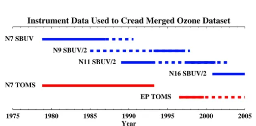
The current MOD total ozone data set includes measurements from 6 satellites: Nim-bus 7 TOMS, NimNim-bus 7 SBUV, NOAA 9, 11, and 16 SBUV/2s, and Earth Probe TOMS. We use the data released by the individual instrument teams, and then apply addi-tional adjustments to each record such that the merged data set is calibrated relative to a reference standard. We use the EP TOMS data from 1996 through mid-1999

15

as the calibration standard, but note that the absolute calibration of the time series is not critical for trend analysis studies. The temporal coverage of the MOD data sets is shown in Fig. 1.

We use the periods denoted by the solid lines to construct the MOD data set. The dashed lines in Fig. 1 represent periods when, though measurements are made, there

20

are calibration or stability issues associated with a given instrument. We compare data in periods of instrument overlap, and use the mean of the differences averaged from 50◦S–50◦N over the available overlap period to determine the adjustment needed to match the standard calibration.

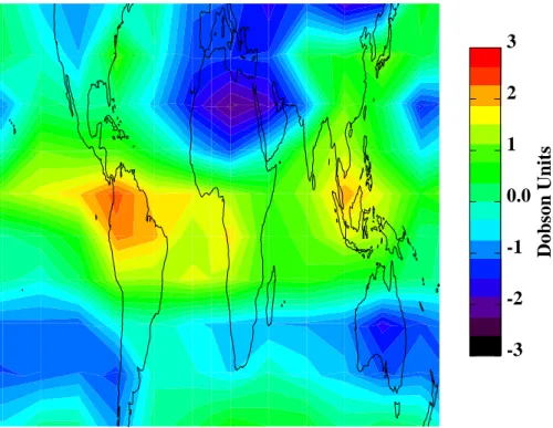
The difference in ozone between two satellites typically shows a characteristic

spa-25

tial distribution, in addition to a simple offset. Figure 2 shows the difference between Nimbus 7 TOMS and Nimbus 7 SBUV grid averages over their 8+ year overlap period.

ACPD

Printer-friendly Version Interactive Discussion Individual instrument gridded-mean maps are created first, and then differenced. Some

of the differences are due to better quality aerosol corrections by the TOMS scanning instrument, as compared to the nadir-only SBUV. Other instrument differences, such as the field of view and orbit precession, can also affect the ozone retrieval and poten-tially lead to systematic differences between the instruments. The interactions within

5

the algorithm are complex, and many of the resulting variations between satellite mea-surements are not understood. To best characterize the overall difference between the data sets, we use the mean of the differences at all longitudes and latitudes between 50◦S and 50◦N. We chose this approach over a latitude-dependent adjustment or an adjustment based on comparisons in a particular region because the differences are

10

not zonal in nature, and we do not understand the distribution well enough to determine which area gives the “correct” bias.

Our first MOD data set was put together in 2000. Fioletov et al. (2002) compared this data to several other satellite and ground-based total ozone data sets and found agreement within 2%. There have since been several modifications, the latest being

15

to include the Version 8 data from TOMS and SBUV (Bhartia et al., 2004). Figure 3 shows the mean comparisons of total ozone as a function of month between different satellites from the Version 7 data and Version 8 data. To compute these differences, 5◦zonal mean monthly time series are constructed for each satellite using all available data. Then in satellite overlap periods, the zonal mean time series are compared (i.e.,

20

space-time match-ups are not required). For each month, the differences in the 5◦zonal means are area weighted and averaged between the latitudes of 50◦S and 50◦N. The external adjustments applied to each record are the average of these differences, as denoted by the thin solid lines. In version 7, a special time-dependent adjustment was made for N7 TOMS, to account for an error that was later corrected in version 8.

25

Note that the V7-based MOD data set included data from the NOAA 14 SBUV/2 instrument, and from NOAA 9 during its overlap period with Nimbus 7 TOMS. These data were deemed by the instrument teams to be of inferior quality, and are not in-cluded in the V8-based data set. The current MOD data set also includes NOAA 16

ACPD

Printer-friendly Version Interactive Discussion data through October 2005. The 2004/2005 NOAA-16 data are provisional, meaning

the complete validation process needed to verify trend-quality data has not been com-pleted. As such, these data are less robust than the data through 2003. Nevertheless, there is nothing in the analysis to date to suggest any shift in calibration that would alter the values of the 2004/2005 data relative to the 2003 data (Matt Deland, personal

5

communication).

The mean differences among the instruments are significantly reduced in the version 8 data set. This is because the development of version 8 algorithm includes a reanaly-sis of the calibration to put all of the satellites on a common reference standard (relative to SSBUV shuttle flight data), reducing the need for additional adjustments (Deland et

10

al., 2004). Although mean adjustments, such as those applied to the V7-based MOD data set, inter-calibrate the data on average, variations due to an instrument calibration error can have a latitude and seasonal dependence (Bhartia et al., 1996). In version 8, the calibration corrections are made to radiance measurements and then propagated through the algorithm, giving a more realistic ozone correction.

15

3 Evaluating instrument uncertainties

When combining multiple satellite records into a long-term data set, we have two sources of error: the long-term drift in each data record, and the spatial pattern of differences between the data sets, which limits our ability to perfectly determine the off-set of one record relative to the other. As seen previously in Fig. 2, differences between

20

satellite measurements often have a characteristic pattern. These differences repre-sent the systematic bias between the two instruments. The standard deviation of the 8-year mean difference pattern between the Nimbus 7 TOMS and SBUV instruments (Fig. 2) was 1 DU.

Figure 4 shows the mean differences between Nimbus 7 TOMS and Nimbus 7 SBUV

25

for the individual years, 1979 and 1986. The difference pattern is similar between the two years (and other years not shown), but there is clearly a year-to-year variability

ACPD

Printer-friendly Version Interactive Discussion about the mean bias. The variability about the bias is also illustrated in Fig. 3 for each

pair of TOMS-SBUV instrument overlaps. This variability and the length of the overlap period give a statistical measure of how precisely we can determine the systematic bias between two instruments. A longer overlap period and/or reduced variability lead to more confidence in the calculated bias, and a reduced offset uncertainty. Therefore

5

the offset uncertainty at any given location is based on the spatial variability of the systematic bias, and our ability to precisely estimate that spatial pattern (the time-dependent variability).

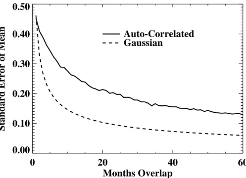
The year-to-year variability about the mean bias is correlated in time, which also affects the uncertainty in the bias estimate. As an example, consider the version 8

10

Nimbus 7 TOMS – Nimbus 7 SBUV monthly difference time series in Fig. 3 (purple curve in right panel). The standard deviation of this difference time series is 0.45 DU. If the data were uncorrelated, the standard error of the mean would decrease rapidly as the square root of the number of months of overlap as shown by the dashed line in Fig. 5. The actual decrease in the uncertainty with additional months of overlap

15

proceeds more slowly because of the auto-correlation of the data, as shown by the solid line in Fig. 5. We fit the overlap difference time series with an auto-regressive lag-1 (ARlag-1) model to derive an estimate of how the uncertainty decreases with increasing overlap. This AR1 model was then used to generate a large number (1000) of time series of a given length. The probability distribution of means for these series was

20

Gaussian and its standard deviation gave the estimate for the non-systematic part of the overlap uncertainty (upper curve in Fig. 5).

The result is an uncertainty of about 0.35 DU for a 5-month overlap, decreasing to about 0.15 DU for a 5-year overlap. For each overlap between satellites, the uncertainty in establishing that relative calibration was estimated as the root sum of squares of two

25

numbers: the statistical uncertainty from Fig. 5 for the number of months of overlap, and the 1.0 DU systematic uncertainty (1.75 DU for the overlap between NOAA 11 and NOAA 16).

ACPD

Printer-friendly Version Interactive Discussion two overlapping instruments, we now consider the possible drift of a single instrument

during its lifetime. We will then combine estimates of the uncertainty in establishing instrument offset and of instrument drift uncertainty to obtain an estimate of overall instrument system drift uncertainty. The instrument drift uncertainty is difficult to as-sess. Herman et al. (1991) did a thorough evaluation of drift uncertainty for the Nimbus

5

7 TOMS during its first decade of measurements. The authors estimated drift uncer-tainty in each component of the calibration for the Nimbus 7 TOMS instrument and propagated these through the entire algorithm process. They estimated a 2σ uncer-tainty of 1.3%/decade or ∼4 DU/decade. In this study, we assume that the Nimbus 7 TOMS drift uncertainty estimate applies to each of the other instruments.

10

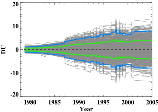
We combine the drift and offset uncertainties by constructing 1000 Monte-Carlo real-izations for the sequence of instruments shown in Fig. 1. The individual realreal-izations are plotted in Fig. 6. The thick green line denotes the standard deviation of the realizations calculated from the distribution at each time step. The blue line indicates two standard deviations.

15

The 2σ instrument uncertainty in the year 2005, according to Fig. 6 is about 8 DU. For the global average ozone amount of about 300 DU, this is 2.7% over 26 years or just slightly more than 1%/decade (∼3 DU/decade). We note that the estimated drift uncertainty is less than that assumed for each individual instrument. Each time a new instrument is added to the time series, the drift from the previous instrument ends, and

20

a new drift begins. Thus the long-term drift is “reset” and the new drift may be in the op-posite direction and partially compensate for the drift in the previous instrument. While these short-term drifts will manifest as correlated noise in the regression analysis, they are not as likely to alias into the long-term trend signal.

4 Trend slow-down detection (CUSUM method)

25

We apply the MOD data set, with uncertainties, to the question of the early detec-tion of column ozone recovery. We use the cumulative sum of residuals (CUSUM),

ACPD

Printer-friendly Version Interactive Discussion in which the cumulative sum of the differences in time between the data and an

as-sumed model is used to characterize the data relative to the model. Reinsel (2002) first used this approach to evaluate changes in ozone trend. He described the method as a “useful graphical device to depict a relatively small change in pattern over time”. Newchurch et al. (2003) expanded on the qualitative approach of Reinsel (2002), using

5

the CUSUM method to quantify and assign significance to an apparent slow-down in the upper stratospheric ozone trend derived from SAGE measurements. They reported a statistically significant reduction in the ozone loss rate globally at 35–45 km altitude. They caution however that evidence of recovery at these altitudes cannot alone be in-terpreted as a recovery of the entire ozone column (Newchurch et al., 2003; WMO,

10

1999). We follow the general approach of Newchurch et al., but we use a different method for assigning significance to the CUSUM results, as detailed below.

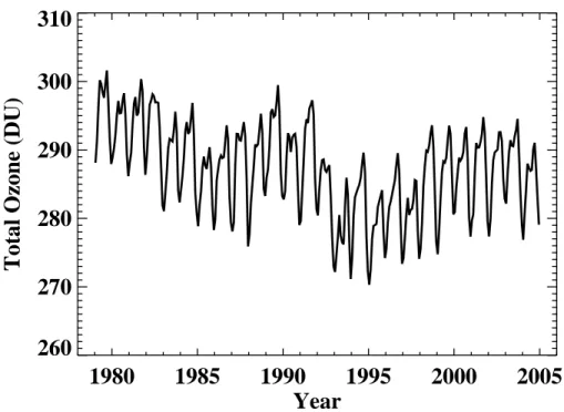
We first apply the technique to a quasi-global average (60◦S–60◦N) MOD time se-ries, shown in Fig. 7. The data generally appear to be increasing since the minimum reached a few years after the Pinatubo volcanic eruption. These data demonstrate the

15

difficulty in separating a possible change in the chemically induced-trend from other natural variations, such as the recovery of ozone after Pinatubo and the upward phase of the solar cycle.

We use our standard statistical time series regression model (Stolarski et al., 2005) to fit the data from 1979 through the end of 1996. We include terms for seasonal

20

cycle, chlorine/bromine, QBO, and solar activity. Here we are fitting the time series only through the end of 1996, so we have replaced the chlorine/bromine term in Sto-larski et al. (2005) with a linear trend. We also add terms to fit the volcanic impacts of Mt. Pinatubo and El Chichon. The volcanic proxies are from the GSFC two-dimensional chemistry and transport mode (2DCTM) approximations of the ozone response to

vol-25

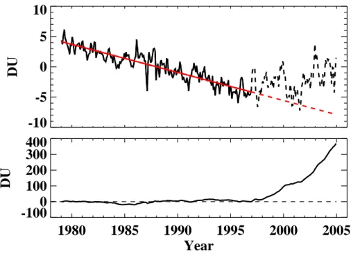
canic aerosols (Stolarski et al., 2006). We then extrapolate the statistical time-series parameters through the end of 2004. The residuals from the fit and its extrapolation are shown in Fig. 8 with the linear trend term added back into the time series for clarity. The red line indicates the linear trend term. The dashed line shows the residuals after

ACPD

Printer-friendly Version Interactive Discussion 1996, the period over which the model fit is extrapolated.

The cumulative sum of residuals is then calculated as the running total of the di ffer-ence between the data anomalies of Fig. 8 and the red line. The bottom panel of Fig. 8 shows the accumulated residuals that rapidly become positive as most of the data is above the extended trend line. Graphically, these results suggest convincing evidence

5

of a trend slowdown, but to assign significance, we must also account for the uncer-tainty of our assumed model. An error in the extrapolated trend due to autocorrelation (statistical error) or drift in the data (instrumental error) would cause an error in the CUSUM that increases with time.

To evaluate the significance of the CUSUM we first determine the statistical

uncer-10

tainty in the trend extrapolation. This uncertainty results from variability not explained by the statistical fit potentially aliasing into the trend term. The residuals are well de-scribed by an auto-regressive time series with lag of one month (AR(1)). The lag one autocorrelation coefficient for the quasi-global time series residuals is 0.53 and the residual white noise is 0.96 DU. The Reinsel (2002) and Newchurch et al. (2003)

stud-15

ies included an AR(1) autocorrelation term in the assumed model, and computed the CUSUM from the white-noise residual. A trend derived from autocorrelated data has a greater uncertainty. Newchurch et al. (2003) scaled the white noise variance by factors designed to account for the greater uncertainty in the model mean value and trend, effectively increasing the value of CUSUM required for statistical significance. In this

20

study, we use a Monte Carlo approach to determine the requirement for significance. We create 1000 random realizations of the residual time series with the same auto-correlation and noise. We then fit a linear trend through the end of 1996, and extrap-olate that trend as our assumed model. The time series realizations have no explicit trend, but may have a non-zero trend through 1996 because of the correlated nature of

25

the noise. The CUSUMs of each of these series are plotted as the gray lines in Fig. 9. By including the autocorrelation in the realizations, we can directly estimate potential errors from statistical model uncertainties in the range of resulting CUSUMS. At each time, the distribution is Gaussian with the 1σ and 2σ variability indicated by the green

ACPD

Printer-friendly Version Interactive Discussion and blue lines respectively. The CUSUM for the data is shown in Fig. 9 as the red line.

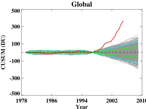
Figure 9 shows a significant trend slow down in the quasi-global time series when only statistical (including autocorrelation) errors are considered. The next step is to include the instrument drift uncertainty for the time series. We again create 1000 artifi-cial time series, each with its own realization of the instrument offset and drift plus the

5

AR(1) autocorrelation and white noise estimated from the data.

Figure 10 shows the CUSUMs for the 1000 artificial time series plotted in gray. Again the green and blue lines indicate the 1σ and 2σ variability in the distributions. When instrument uncertainty is added to the quasi-global data, the overall uncertainty of the resulting CUSUM is significantly increased. The CUSUM of the data shown in red is

10

now only marginally significant at the 2σ level.

The relative impact of instrument uncertainty is less for time series with greater sta-tistical variability, such as zonal average data over smaller latitude ranges. For a time series at a particular location, the instrument drift uncertainty is swamped by the statis-tical uncertainty. Table 1 shows the estimated statisstatis-tical and instrumental uncertainties

15

for four regions of the globe along with the combined uncertainties determined by a root sum of squares. For the quasi-global region (60◦S–60◦N), the total uncertainty is dominated by instrument drift uncertainty. For the mid-latitude regions (30◦N–60◦N and 60◦S–30◦S), the statistical and instrumental uncertainties are comparable.

Figure 11 shows the CUSUM plots for the northern and southern mid-latitudes. The

20

analysis indicates a significant slow down in the trend at northern mid-latitudes, and suggests a slow down in the southern mid-latitudes, but at only the 1.5σ significance level.

We expect that ozone recovery will occur in a predictable spatial pattern in latitude and altitude. Observing recovery that fits this pattern, or fingerprint, gives more

con-25

fidence that we are seeing a true recovery, and not just coincidental results at a few locations. In altitude, initial recovery is expected, and has been reported, in the upper stratosphere (Newchurch et al., 2003).

ACPD

Printer-friendly Version Interactive Discussion a 50-year model simulation (1975–2025) computed using the Goddard 3-D

chemi-cal transport model (Douglass et al., 1997, 2003). The simulation included imposed time-dependent boundary conditions for chlorine- and bromine containing compounds, methane, and nitrous oxide. Solar cycle and volcanic aerosol variations were also in-cluded. Winds and Temperatures used for transport and kinetic reaction calculations

5

were specified using output from a 50-year integration of the Finite-Volume General Circulation Model (FVGCM). Evaluation of model simulations using a prior version of the FVGCM illustrate the credible climatic and transport properties of the model (Stra-han and Douglass, 2004; Considine et al., 2004; Olsen et al., 2004). Further model details can be found in Stolarski et al. (2005).

10

In this study, we apply the CUSUM methodology in the same fashion described above to identify the pattern of ozone recovery in the model. Stolarski et al. (2005) recently completed a statistical time series analysis of this simulation from 1975–2003, and compared the results to the Merged TOMS and SBUV (MOD) data set. On average over the full time period, the model simulation was within 1% of the MOD data, with an

15

offset of less than 3 DU. A larger latitude-dependent average bias was noted, but the mean offset was within 10 DU at all but middle to high southern latitudes. The model simulation was more sensitive to the chlorine/bromine term than was the data. The difference was nearly latitude-independent, with a 1% per decade more negative trend in the model simulations at all latitudes. The difference was slightly larger at high

20

southern latitudes. The CUSUM analysis involves the relative difference between data before and after 1996, and small differences in the absolute sensitivity may also lead to a faster detection of a trend slow-down. We do not believe that it will affect the latitude signature of the expected slow-down as long as the uncertainty in the trend is properly characterized.

25

The uncertainties based on model output for the four regions are shown in Table 2. For consistency we use the same estimate of instrument uncertainty. Stolarski et al. (2005) noted a greater variability in the model simulation at northern mid-latitudes as compared to the MOD data. This increased variability is reflected in the larger

sta-ACPD

Printer-friendly Version Interactive Discussion tistical uncertainties shown in Table 2 for northern mid-latitudes.

The calculated CUSUMs from model data with imposed instrument uncertainties are shown in Fig. 12. The model total ozone indicates a statistically significant trend slow down by 2002 in the mid-latitudes of both hemispheres. The fact that the model has a statistically significant detection of trend slow-down earlier than seen in the data

5

may be a result of the model’s overestimate of sensitivity to chlorine/bromine, or it may suggest that other factors, such as interannual variability, are not fully represented in our statistical model and may be masking the signal of trend slow down in the data. Despite potential differences in timing, we have confidence in the overall spatial pattern of recovery predicted by the model. Therefore, while the data are suggestive, the

10

observations do not yet indicate a statistically significant slow-down in the trend.

5 Summary and conclusions

We have described our method for constructing a merged data set of total column ozone amount. This data set has been available in previous versions on our website athttp://code916.gsfc.nasa.gov/Data services/merged for several years. It has been

15

used in a significant number of papers and has been compared to global data sets put together by others in Fioletov et al. (2002). The newest version extends through 2005 and uses the version 8 TOMS and SBUV data.

In this study we present our first uncertainty analysis of the MOD data set. We account for individual instrument drift uncertainties, and the uncertainty associated

20

with properly combining and adjusting the individual records to a common calibration. We then investigate the impact of the MOD data set uncertainty in trend analyses. We emphasize that individual and merged data sets have uncertainties associated with them. Inclusion of estimates of instrumental uncertainty is crucial to determination of the significance of trends or recovery.

25

We apply our data set with uncertainty estimates to the question of detecting a slow-down of the observed trend in total ozone. We used the cumulative sum (CUSUM)

ACPD

Printer-friendly Version Interactive Discussion method previously employed by Newchurch et al. (2003) with one notable difference.

They included an auto-regressive AR(1) term in their statistical model, and used the white noise residual to compute the CUSUM. To account for possible statistical errors in the extrapolated trend, Newchurch et al. (2003) included additional factors in their significance estimates. In this study, we use a Monte Carlo approach to model the

5

potential impact of statistical errors in the derived trend directly. We include both the autoregressive and white-noise characteristics of the data in many new realizations, and calculate the CUSUM from a trend fit over the period through 1996, then extrap-olated through 2004. The range of resulting CUSUM values give a direct measure of significance requirements.

10

Our results indicate that the slow-down in trend for the quasi-global average (60◦S to 60◦N) has just reached the 2σ significance level. When the data are separated into northern and southern mid-latitude regions, both time series indicate a slowdown in the negative trend. The northern mid-latitude result is significant at the 2σ level, but currently the southern mid-latitude result is only significant at the 1.5σ level. To

15

establish an expected pattern, or “fingerprint” of recovery, we compute the spatial sig-nature of chlorine recovery from a 50-year (1975–2025) simulation using the Goddard 3-D chemical transport model. The model indicates recovery at a similar rate in both hemispheres. At this time, we must conclude that while suggestive, our result fails the fingerprint test for trend slow-down and is therefore not a statistically significant

20

demonstration of the response of total ozone to the leveling off of chlorine.

References

Anderson, J., Russell, J. M., Solomon, S., and Deaver, L. E.: Halogen occultation experiment confirmation of stratospheric chlorine decreases in accordance with the Montreal Protocol, J. Geophys. Res., 105, 4483–4490, 2000.

25

ACPD

Printer-friendly Version Interactive Discussion

for the estimation of vertical ozone profiles from the backscattered ultraviolet technique, J. Geophys. Res., 101, 18 793–18 806, 1996.

Bhartia, P. K., McPeters, R. D., Stolarski, R. S., Flynn, L. E., and Wellemeyer, C. G.: A quarter century of ozone observations by SBUV and TOMS, Proceedings of the XX Quadrennial Ozone Symposium, Kos, 1–8 June, Greece, 2004.

5

Considine, D. B., Douglass, A. R., Connell, P. S., Kinnison, D. E., and Rotman, D. A.: A po-lar stratospheric cloud parameterization for the global modeling initiative three-dimensional model and its response to stratospheric aircraft, J. Geophys. Res., 105, 3955–3973, 2000. Deland, M. T., Huang, L.-K., Taylor, S. L., McKay, C. A., Cebula, R. P., Bhartia, P. K., and

McPeters, R. D.: Long-term SBUV and SBUV/2 instrument calibration for Version 8 data, 10

Proceedings of the XX Quadrennial Ozone Symposium, Kos, 1–8 June, Greece, 2004. Douglass, A. R., Rood, R. B., Kawa, S. R., and Allen, D. J.: A three-dimensional simulation

of the evolution of the middle latitude winter ozone in the middle stratosphere, J. Geophys. Res., 102, 19 217–19 232, 1997.

Douglass, A. R., Schoeberl, M. R., Rood, R. B., and Pawson, S.: Evaluation of transport in 15

the lower tropical stratosphere in a global chemistry and transport model, J. Geophys. Res., 108, 4259, doi:10.1029/2002JD002696, 2003.

Fioletov, V. E., Bodeker, G. E., Miller, A. J., McPeters, R. D., and Stolarski, R.: Global and zonal total ozone variations estimated from ground-based and satellite measurements: 1964– 2000, J. Geophys. Res., 107, 4647, doi:10.1029/2001JD001350, 2002.

20

Herman, J. R., Hudson, R., McPeters, R., Stolarski, R., Ahmad, Z., Gu, X. Y., Taylor, S., and Wellemeyer, C.: A new self-calibration method applied to TOMS and SBUV backscattered ultraviolet data to determine long-term global ozone change, J. Geophys. Res., 96, 7531– 7545, 1991.

Montzka, S. A., Butler, J. H., Elkins, J. W., Thompson, T. M., Clarke, A. D., and Lock, L. T.: 25

Present and future trends in the atmospheric burden of ozone-depleting substances, Nature, 398, 690–694, 1999.

Montzka, S. A., Butler, J. H., Hall, B. D., Mondeel, D. J., and Elkins, J. W.: A decline in trop-sopheric organic bromine, Geophys. Res. Lett., 30(15), 1836, doi:10.1029/2003GL017745, 2003.

30

Newchurch, M. J., Yang, E.-S., Cunnold, D. M., Reinsel, G. C., Zwodny, J. M., and Russell III, J. M.: Evidence for slowdown in stratospheric ozone loss: First stage of ozone recovery, J. Geophys. Res., 108, 4507, doi:10.1029/2003JD003471, 2003.

ACPD

Printer-friendly Version Interactive Discussion

Olsen, M. A., Schoeberl, M. R., and Douglass, A. R.: Stratosphere-Troposphere Exchange of Mass and Ozone, J. Geophys. Res., 109, 24114, doi:10.1029/2004JD005186, 2004. Reinsel G. C.: Trend analysis of upper stratospheric Umkehr ozone data for evidence of

turnaround, Geophys. Res. Lett., 29, 1451, doi:10.1029/2002GL014716, 2002.

Rinsland, C. P., Mathieu, E., Zander, R., Jones, N. B., Chipperfield, M. P., Goldman, A., Ander-5

son, J., Russell, J. M., Demoulin, P., Notholt, J., Toon, G. C., Blavier, J. F., Sen, B., Sussmann, R., Wood, S. W., Meier, A., Griffith, D. W. T., Chiou, L. S., Murcray, F. J., Stephen, T. M., Hase, F., Mikuteit, S., Schulz, A., and Blumenstock, T.: Long-term trends of inorganic chlorine from ground-based infrared solar spectra: Past increases and evidence for stabilization, J. Geo-phys. Res., 108, 4252, doi:10.1029/2002JD003001, 2003.

10

Staehelin, J., Harris, N. R. P., Appenzeller, C., and Eberhard, J.: Ozone trends: A review, Rev. Geophys., 39, 231–290, 2001.

Strahan, S. E. and Douglass, A. R.: Evaluating the credibility of transport processes in sim-ulations of ozone recovery using the Global Modeling Initiative three-dimensional model, J. Geophys. Res., 109, 05110, doi:10.1029/2003JD004238, 2004.

15

Stolarski, R., Bojkov, R., Bishop, L., Zerefos, C., Staehelin, J., and Zawodny, J.: Measured trends in stratospheric ozone, Science, 256, 342–349, 1992.

Stolarski, R. S., Douglass, A. R., Steenrod, S., and Pawson, S.: Trends in Stratospheric ozone: lessons learned from a 3D chemical transport model, J. Atmos. Sci., 63, 1028–1041, 2006. Taylor, S. L., Cebula, R. P., Deland, M. T., Huang, L. K., Stolarski, R. S., and McPeters, R. 20

D.: Improved calibration of NOAA-9 and NOAA-11 SBUV/2 total ozone data using in-flight validation methods, Int. J. Remote Sens., 24, 315–328, 2003.

WMO (World Meteorological Organization): Scientific Assessment of Ozone Depletion: 1998, Global Ozone Research and Monitoring Project-Report No. 44, Geneva, 1999.

WMO (World Meteorological Organization): Scientific Assessment of Ozone Depletion: 2002, 25

ACPD

Printer-friendly Version Interactive Discussion Table 1. Data uncertainties in DU/decade.

Region Statistical Instrumental Total Global (60◦S–60◦N) 0.9 3.0 3.1 N Midlat (30◦N–60◦N) 3.7 3.0 4.8 S Midlat (60◦S–30◦S) 3.8 3.0 4.9 Tropical (30◦S–30◦N) 1.4 3.0 3.3

ACPD

Printer-friendly Version Interactive Discussion Table 2. Model statistical uncertainties in DU/decade with instrument uncertainty.

Region Statistical Instrumental Total Global (60◦S–60◦N) 0.9 3.0 3.1 N Midlat (30◦N–60◦N) 5.6 3.0 6.2 S Midlat (60◦S–30◦S) 3.4 3.0 4.6 Tropical (30◦S–30◦N) 1.4 3.0 3.3

ACPD

Printer-friendly Version Interactive Discussion Instrument Data Used to Cread Merged Ozone Dataset

1975 1980 1985 1990 1995 2000 2005 Year N7 SBUV N9 SBUV/2 N11 SBUV/2 N16 SBUV/2 N7 TOMS EP TOMS

Fig. 1. Instruments used to create merged ozone data set. Solid lines indicate time when

data was used. Dashed lines indicate time when data was available, but not used for reasons explained in the text.

ACPD

Printer-friendly Version Interactive Discussion -3 -2 -1 0.0 1 2 3 Dobson Units

Fig. 2. Difference between Nimbus 7 TOMS and Nimbus 7 SBUV measurements for total ozone

ACPD

Printer-friendly Version Interactive Discussion

V7

1980

1985

1990

1995

2000

Year

-10

-8

-6

-4

-2

0

2

4

TOMS-SBUV (DU)

V8

1980

1985

1990

1995

2000

Year

Fig. 3. The two panels show the inter-instrument comparisons (TOMS-SBUV) for all available

overlap periods plotted as a function of time. Version 7 data are shown in the left panel and version 8 data in the right panel. The plotted differences are averaged from 50◦N–50◦S. We use these differences to determine the best offsets to apply to each data set in order to create an internally consistent calibration for the MOD data set.

ACPD

Printer-friendly Version Interactive Discussion

1979

1986

-3

-2

-1

0.0

1

2

3

Dobson Units

Fig. 4. Difference between Nimbus 7 TOMS and Nimbus 7 SBUV measurements of total ozone

ACPD

Printer-friendly Version Interactive Discussion

0

20

40

60

Months Overlap

0.00

0.10

0.20

0.30

0.40

0.50

Standard Error of Mean

Auto-Correlated

Gaussian

Fig. 5. Statistical uncertainty in establishing systematic bias between Nimbus 7 TOMS and

Nimbus 7 SBUV as a function of the number of months overlap. Solid line is uncertainty with auto-correlation taken into account. Dashed line is standard error of the mean if data were uncorrelated.

ACPD

Printer-friendly Version Interactive Discussion

1980

1985

1990

1995

2000

2005

Year

-20

-10

0

10

20

DU

Fig. 6. Instrument drift uncertainty vs. time for MOD. Green line indicates 1σ uncertainty and

ACPD

Printer-friendly Version Interactive Discussion

1980

1985

1990

1995

2000

2005

Year

260

270

280

290

300

310

Total Ozone (DU)

ACPD

Printer-friendly Version Interactive Discussion

-10

-5

0

5

10

DU

1980

1985

1990

1995

2000

2005

Year

-100

0

100

200

300

400

DU

Fig. 8. Top: residuals from time-series fit to quasi-global MOD time series with

annually-averaged linear trend added back in. Dashed line is the extension of the residuals beyond to fitting time period of 1979–1996. Red line is the linear fit term. Bottom: cumulative sum of residuals from top panel as a function of time.

ACPD

Printer-friendly Version Interactive Discussion

Global

1978

1986

1994

2002

2010

Year

-500

-300

-100

100

300

500

CUSUM (DU)

Fig. 9. Cumulative sum results without inclusion of instrument uncertainty. The gray region is

formed by line plots of 1000 monte-carlo cases used to determine uncertainty. The green thick line is the 1σ width of the probability distribution of the 1000 cases as a function of time. The light blue line is the 2σ width of the distribution. The red line is the cumulative sum of residuals for the data.

ACPD

Printer-friendly Version Interactive Discussion

Global

1978

1986

1994

2002

2010

Year

-500

-300

-100

100

300

500

CUSUM (DU)

Fig. 10. Same as Fig. 9 with the uncertainty due to possible drift in the instrument record

ACPD

Printer-friendly Version Interactive Discussion 1978 1986 1994 2002 2010 Year -1000 -500 0 500 1000 CUSUM (DU) 30o N-60o N 1978 1986 1994 2002 2010 Year 30o S-60o S

Fig. 11. Cumulative sum of residuals for the northern mid-latitudes (30◦–60◦N) in left panel, and southern mid-latitudes (30◦–60◦S) in right panel. Definition of lines is the same as Fig. 10.

ACPD

Printer-friendly Version Interactive Discussion 1978 1986 1994 2002 2010 Year -1000 -500 0 500 1000 CUSUM (DU) 30oN-60oN 1978 1986 1994 2002 2010 Year 30oS-60oS

Fig. 12. Model fingerprint of ozone trend slow-down expressed in CUSUM terms. The northern

mid-latitudes (30◦–60◦N) are shown in the left panel; the southern mid-latitudes (30◦–60◦S) are shown in the right panel.