HAL Id: insu-01398530
https://hal-insu.archives-ouvertes.fr/insu-01398530
Submitted on 25 Nov 2016
HAL is a multi-disciplinary open access
archive for the deposit and dissemination of
sci-entific research documents, whether they are
pub-lished or not. The documents may come from
teaching and research institutions in France or
abroad, or from public or private research centers.
L’archive ouverte pluridisciplinaire HAL, est
destinée au dépôt et à la diffusion de documents
scientifiques de niveau recherche, publiés ou non,
émanant des établissements d’enseignement et de
recherche français ou étrangers, des laboratoires
publics ou privés.
of the Arctic atmospheric boundary layer around
Spitsbergen compared to ERA-Interim and Arctic
System Reanalyses
Tjarda J. Roberts, Marina Dütsch, Lars R. Hole, Paul B. Voss
To cite this version:
Tjarda J. Roberts, Marina Dütsch, Lars R. Hole, Paul B. Voss. Controlled meteorological (CMET)
free balloon profiling of the Arctic atmospheric boundary layer around Spitsbergen compared to
ERA-Interim and Arctic System Reanalyses. Atmospheric Chemistry and Physics, European Geosciences
Union, 2016, 16 (19), pp.12383-12396. �10.5194/acp-16-12383-2016�. �insu-01398530�
www.atmos-chem-phys.net/16/12383/2016/ doi:10.5194/acp-16-12383-2016
© Author(s) 2016. CC Attribution 3.0 License.
Controlled meteorological (CMET) free balloon profiling of the
Arctic atmospheric boundary layer around Spitsbergen compared
to ERA-Interim and Arctic System Reanalyses
Tjarda J. Roberts1,2, Marina Dütsch3,4, Lars R. Hole3, and Paul B. Voss5
1LPC2E/CNRS, 3A, Avenue de la Recherche Scientifique, 45071 Orléans, CEDEX 2, France 2Norwegian Polar Institute, Fram Centre, 9296 Tromsø, Norway
3Norwegian Meteorological Institute, Bergen, Norway
4Institute for Atmospheric and Climate Science, ETH Zurich, 8092 Zurich, Switzerland 5Smith College, Picker Engineering Program, Northampton, MA, USA
Correspondence to:Tjarda J. Roberts (tjardaroberts@gmail.com)
Received: 22 May 2015 – Published in Atmos. Chem. Phys. Discuss.: 14 October 2015 Revised: 4 July 2016 – Accepted: 18 July 2016 – Published: 30 September 2016
Abstract. Observations from CMET (Controlled Meteo-rological) balloons are analysed to provide insights into tropospheric meteorological conditions (temperature, hu-midity, wind) around Svalbard, European High Arctic. Five Controlled Meteorological (CMET) balloons were launched from Ny-Ålesund in Svalbard (Spitsbergen) over 5–12 May 2011 and measured vertical atmospheric profiles over coastal areas to both the east and west. One notable CMET flight achieved a suite of 18 continuous soundings that probed the Arctic marine boundary layer (ABL) over a period of more than 10 h. Profiles from two CMET flights are compared to model output from ECMWF Era-Interim reanal-ysis (ERA-I) and to a high-resolution (15 km) Arctic System Reanalysis (ASR) product. To the east of Svalbard over sea ice, the CMET observed a stable ABL profile with a temper-ature inversion that was reproduced by ASR but not captured by ERA-I. In a coastal ice-free region to the west of Svalbard, the CMET observed a stable ABL with strong wind shear. The CMET profiles document increases in ABL temperature and humidity that are broadly reproduced by both ASR and ERA-I. The ASR finds a more stably stratified ABL than observed but captured the wind shear in contrast to ERA-I. Detailed analysis of the coastal CMET-automated sound-ings identifies small-scale temperature and humidity varia-tions with a low-level flow and provides an estimate of local wind fields. We demonstrate that CMET balloons are a valu-able approach for profiling the free atmosphere and boundary
layer in remote regions such as the Arctic, where few other in situ observations are available for model validation.
1 Introduction
In remote regions such as the Arctic there exists very limited in situ observational data to evaluate atmospheric models. This study demonstrates CMET (Controlled Meteorological) balloons as a new approach for detailed probing of the Arctic atmospheric boundary layer on local-to-regional scales and compares the observations to model reanalysis outputs.
Accurate representation of polar meteorology and small-scale air–sea ice interaction processes is essential for me-teorological forecast models and to understand climate in the Arctic, a region undergoing rapid change (Vihma et al., 2014). The atmospheric boundary layer in the Arctic is usu-ally strongly stable during winter and only weakly stable to neutral during summer (Persson et al., 2002). Strong temper-ature inversions can occur as warmer air masses from lower latitudes are advected over the cold polar air masses. This stability acts as a barrier to vertical atmospheric mixing and exchange and can magnify flows over small-scale topogra-phy such as channelling and katabatic flows. The Barents Sea near Svalbard is especially implicated in Arctic climate (Smedsrud et al., 2013). To the east of Svalbard, the Barents Sea is typically partially covered by sea ice during winter and
spring, whilst sea ice is typically absent in the Greenland Sea to the west of Svalbard. This is due to the northward flow-ing warm and saline Atlantic Warm Current (AWC) or North Atlantic Drift, which elevates temperatures along Svalbard’s west coast, with a secondary branch that enters the Barents Sea. The warm saline AWC releases heat to the atmosphere as it cools to sink beneath the polar waters. The polar wa-ters experience thermodynamic formation, growth and melt of sea ice as well as wind- and oceanic-current-driven ad-vection of sea ice, which can lead to highly variable surface conditions that affect air–sea exchange of heat and momen-tum and the radiative balance, e.g. through albedo. Even at high sea ice density, small patches of open water amongst very close (90–100 %) or close (80–90 %) drift ice tend to promote sea–air exchange, enhancing both temperature and specific humidity at the surface (Andreas et al., 2002). Con-versely, snow deposited upon sea ice provides an insulating layer that reduces heat exchange. Hence, heat and energy fluxes to the Arctic atmospheric boundary layer can vary by several orders of magnitude, depending on the surface state (Kilpeläinen et al., 2011).
Model reanalyses provide temporally consistent represen-tations of atmospheric and surface state and are a valu-able tool for understanding Arctic processes and climate. A global model reanalysis product is ERA-Interim (ERA-I) from the European Centre for Medium-Range Weather Fore-casts (ECMWF), Dee et al. (2011). At approximately 80 km resolution, ERA-I has been widely used including for Arc-tic studies, e.g. Rinke et al. (2006). Recently, ArcArc-tic System Reanalysis (ASR) products have been developed at higher resolution (15–30 km) and specifically focused on high lat-itudes (Bromwich et al., 2016). There is an ongoing effort to validate and compare the ASR and ERA-I reanalyses data sets. The ASR (version 1: 30 km resolution) and ERA-I re-analyses exhibit comparable RMS errors for surface meteo-rology compared to Arctic-wide collated meteorological sta-tion data (December 2006–November 2007), (Bromwich et al., 2016). Wind speed biases were significantly smaller in the ASRv1. North of 60◦N, ASRv1 showed smaller precip-itation biases than ERA-I except during summer. Moore et al. (2015) showed that the higher-resolution ASRv1 is more able to fully resolve mesoscale features in the atmosphere, such as katabatic wind, to the south-east of Greenland, com-pared to ERA-I. Wesslén et al. (2014) comcom-pared ASRv1 and ERA-I reanalyses to surface and radiosonde meteorological data obtained during a 3-week ice drift experiment in sum-mer 2008, a period typically influenced by clouds. ERA-I was found to have a systematic warm bias in the lowest tro-posphere, whilst ASRv1 had a systematic cold bias of similar magnitude. The ASR version 2 at 15 km resolution has re-cently been developed. Moore et al. (2016) demonstrate the added value of ASRv2 compared to ASRv1 in resolving to-pographically forced winds and capturing mesoscale spatial features around Greenland due to the higher resolution.
In this study we compare ASRv2 (at 15 km resolution) and ERA-I to in situ CMET balloon observations in the Sval-bard region during the 2011 Arctic spring. In this region in situ measurements of the boundary layer and lower tro-posphere are limited. Meteorological stations provide con-tinuous ground-based data and regular daily meteorological balloon profiles, but are sparsely located. In Svalbard, such data sets may be occasionally supplemented by tethered bal-loon or meteorological mast observations (e.g. Mäkiranta et al., 2011). Intensive field campaigns probe more remote re-gions of the Arctic by aircraft (e.g. Vihma et al., 2005) or by drifting ice stations (e.g. Rinke et al., 2006, Tjernström et al., 2012), but these can only be rarely undertaken due to cost. Remotely piloted aircraft systems (RPAS) also known as un-manned aerial vehicles (UAV) equipped with meteorological sensors provide an alternative cost-effective means to spa-tially probe the Arctic boundary layer around Svalbard at lo-cal slo-cales, Mayer et al. (2012a, b). However, most UAVs are operated over timescales up to a few hours and over ranges typically limited to a few 10s of km. For low-altitude flights the range may be further limited if terrain blocks the signal.
To provide an in situ meteorological data set that sam-ples the wider Svalbard Arctic region we deployed five Con-trolled Meteorological (CMET) balloons, launched in May 2011 from Ny-Ålesund in Svalbard. CMET balloons are ca-pable of performing sustained flights within the troposphere at designated altitudes and can make vertical soundings at any time during the balloon flight on command via satellite link (Voss et al., 2012). The nested dual balloon design en-sures very little helium loss, enabling the balloons to make multi-day flights. This gives an opportunity to investigate ar-eas far away from research bases, at greater spatial scales (many hundreds of kilometres from the launch point) than can be obtained by line-of-sight RPAS/UAV approaches, ra-diosondes or tethered balloons. The study builds upon pre-vious uses of CMET balloons to probe regional-scale me-teorology including atmospheric trajectories (Riddle et al., 2006), air flow downwind from a city pollution source (Voss et al., 2010) and Antarctic meteorology on local-to-regional scales (Stenmark et al., 2014; Hole et al., 2016). Here we demonstrate the capability of CMET balloons to repeatedly make in-flight soundings down to low altitudes that reach into the atmospheric boundary layer. We present multiple CMET flights of long duration (up to several days) in the Arctic including a CMET configured to make automated con-tinuous profiling into the atmospheric boundary layer. These CMET in situ profiles of temperature, humidity and wind are compared to ERA-I and ASR model reanalyses.
2 Methods
2.1 CMET balloon and payload description
Controlled Meteorological (CMET) balloons can fly for mul-tiple days in the troposphere with altitude controlled via satellite link (Voss et al., 2012). Altitude control is achieved by the dual balloon design (high-pressure inner and low-pressure outer balloon) between which helium is transferred by a miniature pump–valve system. Commands sent through an Iridium satellite link can set target altitude (typically 0– 3500 m), control band (∼ 50–500 m with the higher band us-ing less power), vertical velocity (∼ 0.5–1.5 m s−1), termi-nation countdown timer and numerous other operational pa-rameters. For this study, a new capacity was added to per-form automated soundings between two specified pressure altitudes.
The 215 g CMET payload (excluding balloon envelopes) includes the control electronics, GPS receiver, satellite mo-dem, pump-valve system, lithium polymer battery, photo-voltaic panel, aspirated T-RH sensor and a vacuum-insulated pouch for the payload. The payload temperature is main-tained within acceptable operating limits (typically +20◦C above ambient) even at altitudes of several kilometres in the Arctic.
An aviation-grade pressure sensor (Freescale MPXH6115A) coupled to a 16 bit analog-to-digital converter (Analog Devices AD7795) provides altitude information to the balloon’s control algorithm every 10 s during flight. As part of data post-processing, this pressure-derived altitude is corrected for pressure offsets using the in-flight GPS altitude (Inventek ISM300X). GPS latitude and longitude provide the in-flight CMET coordinates and are also further analysed during flight to determine wind speeds in eastward (U ) and northward (V ) directions.
Temperature is measured using a thermistor (General Electric MC65F103A) in a 10 k-Ohm divider circuit coupled to the aforementioned analog-to-digital converter. A capaci-tance humidity sensor (G-TUCN.34 from UPSI, covering 2 to 98 % RH range over −40 to +85◦C) generates a signal which is a function of the ambient relative humidity (RH) with respect to water. Relative humidity was converted to specific humidity (Q) for comparison to the ERA-I and ASR model outputs.
CMETs are relatively simple to launch (requiring just 1–2 people with standard meteorological balloon skills: launches have been achieved under a wide range of surface winds to date) and are similar in size to a standard meteorologi-cal balloon. Further details of the CMET balloon, payload design and balloon flight engineering are described by Voss et al. (2012) and illustrated at http://www.science.smith.edu/ cmet/flight.html.
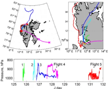
Figure 1. Trajectories of five CMET balloons launched from Ny-Ålesund in May 2011. Flight paths are shown on the regional scale of the island Spitsbergen, Svalbard and on the local scale of Kongs-fjord. Ny Ålesund is marked by a yellow circle and lies at the south-ern side of Kongsfjord. Balloons 4 and 5 performed repeated sound-ings as shown by the pressure variations in time (marked *). Anal-ysis periods for flights 4 (06:00–12:00 UTC) and 5 (full flight) are denoted by x.
2.2 Balloon launches in Svalbard
Five CMET balloons were launched from the research sta-tion of the Alfred Wegener Institute and the Polar Institute Paul Emile Victor (AWIPEV) in Ny Ålesund, over the pe-riod 5 to 12 May 2011 (JD 125 to 132) (Fig. 1). Balloons 1 and 2 had short flights due to technical issues encoun-tered at the start of the campaign. Balloon 3 flew far north and was the longest duration flight in this campaign but did not perform any soundings after leaving the coastal area of Svalbard. Balloon 4 flew eastwards, but despite good bal-loon performance needed to be terminated before encroach-ing Russian airspace. It performed two closely spaced (as-cent and des(as-cent) soundings over sea ice in the Barents Sea, east of Svalbard. Balloon 5 undertook a 24 h duration flight that first exited Kongsfjorden, then flew northwards along the coast. It was placed into an automated sounding mode and achieved a much longer series of 18 consecutive profiles of the ABL, before being raised to higher altitudes where winds advected it eastwards. To the best of our knowledge, this was the first demonstration of a set of extended controlled sound-ings made using a free balloon.
The data analysis of this study focuses on balloon flights 4 and 5, which made repeated soundings quantifying the following meteorological variables as a function of pres-sure (altitude): temperature (T ), specific humidity (Q) and northward and eastward winds (V , U ). The balloon locations during these flights are shown in Fig. 1. A detailed model
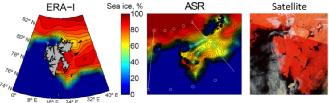
Figure 2. Sea ice concentration field on 8 May (JD 128) in ERA-I and ASR reanalyses. The ERA-I image shows a map of Svalbard overlain. The ERA-I map coordinates are depicted on the ASR image for ease of comparison. Also shown is the Lance rapid response image (right) from the MODIS satellite (downloaded from http://lance-modis.eosdis.nasa.gov/, land and sea ice are shown in red, cloud cover in white) for 5 May 2011 (JD 125).
comparison is made for flight 4 over time periods 06:00– 12:00 UTC on 8 May (JD 128) and for the 24 h flight 5 (21:00–21:00 UTC) on 10–11 May (JD 130-131).
2.3 Model reanalyses products ERA-I and ASR The CMET observations are compared to two model re-analyses: ECMWF ERA-Interim (Dee et al., 2011) and the Arctic System Reanalysis (Bromwich et al., 2016). ERA-I (available from http://apps.ecmwf.int/) has approximately 80 km (T255 spectral) resolution on 60 vertical model levels from the surface up to 0.1 hPa, at 6-hourly resolution. The boundary layer and lower troposphere (> ∼ 800 hPa) corre-spond to 14 model levels. For this study, bilinearly interpo-lated model level data were downloaded at 0.125◦ spatial resolution, then further linearly interpolated. ASR uses the polar-optimized version of the Weather Research and Fore-casting Model (Polar-WRF: Bromwich et al., 2009) with an inner domain that extends over latitudes > 40◦N, using ERA-I output as boundary conditions. ASR (version 2) has 15 km resolution on 70 vertical model levels from the sur-face up to 0.1 hPa, at 3-hourly resolution (ASR version 1 at 30 km resolution is used in this study only for compari-son to a surface station). The boundary layer and lower tro-posphere (> ∼ 800 hPa) correspond to 30 model levels. For this study, full ASRv2 model level data were made specially available by the ASR team for selected field dates. Pressure-level data for ASRv2 will soon be publicly available from http://rda.ucar.edu/. The ASR and ERA-I reanalyses were 4-D (latitude, longitude, pressure and time) interpolated to the CMET balloon for direct comparison. A main difference be-tween these two reanalyses is the much higher temporal (3-hourly) and spatial (15 km) resolution of ASR. This provides a more highly resolved simulation of small-scale meteoro-logical processes (especially within the boundary layer) as well as topography. Another difference is that ASR Polar WRF has non-hydrostatic dynamics whilst ERA-I pressure is hydrostatic. Both model reanalyses include assimilation of remotely sensed retrievals and in situ surface and upper
air data, 4-D for ERA-I and 3-D for ASR. ASR uses a high-resolution land data assimilation system and uses Polar WRF which includes the Noah land surface model and a detailed fractional sea ice description including extent, concentration, thickness, albedo and snow cover (see Bromwich et al., 2016 for details). For ERA-I surface properties are less detailed (spatio-temporally) than for ASR, but sea ice is also frac-tional and updated daily.
Sea ice concentration in ERA-I and ASR models is shown in Fig. 2 for 8 May (JD 128), the date of the CMET flight 4 soundings. Also shown is a satellite image of sea ice cover-age (obtained for 5 May, JD 125). The west of Svalbard is ice-free, consistent with sea-surface temperature in this re-gion (see Introduction), whilst dense sea ice occurs east of Svalbard. The satellite image also shows some small-scale features in ice-free areas (polynyas). These are not seen in the ERA-I ice-field but are represented in ASR as zones of lower ice concentration.
3 Results and discussion
3.1 Meteorological conditions during the campaign The period of 5–12 May 2011 was characterized by rapidly changing meteorological conditions, reflected in the different CMET flight paths (Fig. 1). The time evolution of the pres-sure systems driving the winds that advected the CMETs is illustrated by ERA-I model surface pressure maps in Fig. 3. The start of the campaign is influenced by a high-pressure system that slowly advected balloon 3 northwards. A low-pressure system then developed to the north and east of Sval-bard, which is responsible for the south-eastwards advection of balloon 4. Presence of a high-pressure system causes a slow northwards, followed by an eastwards advection of bal-loon 5. Surface observations (resolution in minutes) from the AWIPEV meteorological station in Ny-Ålesund (Maturilli et al., 2013) are shown alongside the ERA-I and ASR model outputs in Fig. 4. The greatest wind speeds during the
cam-125 0 20 40 75 80 85 125.5 0 20 40 75 80 85 126 0 20 40 75 80 85 126.5 0 20 40 75 80 85 127 0 20 40 75 80 85 127.5 0 20 40 75 80 85 128 0 20 40 75 80 85 128.5 0 20 40 75 80 85 129 0 20 40 75 80 85 129.5 0 20 40 75 80 85 130 0 20 40 75 80 85 130.5 0 20 40 75 80 85 131 0 20 40 75 80 85 131.5 0 20 40 75 80 85 132 0 20 40 75 80 85 132.5 0 20 40 75 80 85
ERA−I Sea Level Pressure, hPa
11000000 1005 1010 1015 1020 1025 1030 1035 N J. day E o o 1000 1005 1010 1015 1020 1025 1030 1035
ERA-I sea-level pressure, hPa
Figure 3. Sea-level pressure in ERA-I shown as a function of lat-itude and longlat-itude at 12-hourly intervals for the duration of the field campaign, starting on JD 125 (5 May). Overlain in white are Ny-Ålesund and the CMET flight tracks as a function in time (full extents of flights 3 and 4 are shown at JD 128.5 and for flight 5 at JD 132).
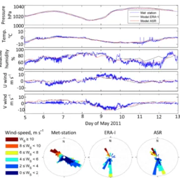
paign are observed on 8–10 May with the AVIPEV station registering a maximum wind speed of 17.4 m s−1 around noon on 9 May. During this period the winds became north-westerly due to the presence of a high-pressure system SW and a lower-pressure system NE of Svalbard. This caused temperature to decrease during this period. This was fol-lowed by a period of low wind speed over 11–12 May, also reflected in the 24 h CMET flight to the east of Svalbard, with low but increasing temperatures recorded at the meteorolog-ical station. Both models show good general agreement with the Ny-Ålesund surface meteorological observations of 2 m temperature, relative humidity and surface pressure (Fig. 4). This is not entirely unexpected given the use of data assim-ilation in both reanalyses. The models reproduced the vari-ation in 10 m wind speed, but not always the wind direction reported at AWI-PEV (Fig. 4). This is likely due to known along-fjord wind channelling in the Kongsfjorden that oc-curs on finer scales than the resolution of the reanalyses. In-deed, Esau and Repina (2012) found that even a very fine-resolution model (56 × 61 m grid cell) could not fully resolve near-surface small-scale turbulence in the strongly stratified Kongsfjorden atmosphere, where the valley is surrounded by steep mountain topography.
Figure 4. Meteorology parameter time series (resolution in min-utes) from the Ny-Ålesund AWIPEV station compared to ERA-I (6-hourly) and ASR (3-hourly) outputs for pressure, temperature, relative humidity, U and V winds. Wind roses compare modelled and observed wind directions.
3.2 CMET profiles over sea ice compared to ERA-I and ASR: temperature inversion
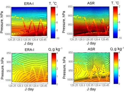
The two consecutive CMET profiles of temperature, specific humidity, U and V winds over sea ice east of Svalbard (bal-loon flight 4) on the morning of JD 128 are compared to 4-D interpolated ERA-I and ASR model data (Figs. 5 and 6). The in-flight CMET soundings quantify temperature and humid-ity profiles which increase towards the surface as expected, as well as winds (derived from the balloon flight path) from the north-west. There is good general agreement with ASR and ERA-I. However, the CMET observes a temperature in-version at around 990–970 hPa which persists for most of the sounding time series. This temperature inversion is captured by ASR in good agreement with the CMET but is not repro-duced by ERA-I. ASR finds a strong gradient in humidity related to this inversion barrier, but the CMET observes a more shallow humidity gradient. ERA-I finds an even shal-lower gradient in humidity than the CMET. Both models show strengthening westerly winds during the soundings, as observed. The CMET observed a reversal in V winds near the surface (> 1000 hPa). This is better captured by ASR than ERA-I, where it is related in the model to the inversion layer. However, there are differences in V winds at higher altitudes, which are more variable in ASR than in the CMET and ERA-I.
The potential temperature and specific humidity profiles from the CMET flight are further shown in Fig. 7, alongside
Figure 5. Temperature and specific humidity measured during the CMET flight 4 soundings (filled circles) compared to 4-D interpolated (latitude, longitude, pressure, time) model data from ERA-I and ASR.
Figure 6. U and V winds observed during the CMET flight 4 soundings (filled circles) compared to 4-D interpolated (latitude, longitude, pressure, time) model data from ERA-I and ASR.
equivalent 4-D interpolated model outputs at each CMET latitude, longitude, pressure and time location. The CMET potential temperature profile shows two distinct layers: a strongly stable layer between 990 and 970–980 hPa (re-lated to the abovementioned inversion) and a stable layer <980 hPa. This agrees well with similar layers identified in the ASR, whereas the absence of an inversion layer in ERA-I leads to a more linear potential temperature profile.
The specific humidity profile of ASR shows better agreement with CMET at ∼ 980 hPa, whereas ERA-I overestimates it by 0.2 g kg−1. At higher altitudes, ERA-I is in better agreement whilst ASR shows greater humidity variability (overestima-tions by up to 0.3 g kg−1) than the trend observed by CMET. It is difficult to infer any temporal trend in the flight 4 CMET profiles over the morning of JD 128. The final pro-file (JD > 128.45) shows slightly greater humidity at low
al-Figure 7. Profiles of potential temperature and specific humidity during flight 4 as observed by the CMET balloon and according to the 4-D interpolated ERA-I and ASR model outputs.
titudes but also slightly lower temperature and the inversion is less clear. ERA-I and ASR show a tendency for increasing surface temperature and humidity. In the morning ASR pdicts a deepening layer beneath the inversion, but the top re-mains at constant height. Unfortunately the experiment could not be continued eastwards into the afternoon as the CMET flight had to be terminated to avoid Russian airspace. 3.3 CMET profiles in coastal area compared to ERA-I
and ASR: wind shear and temperature and humidity trends
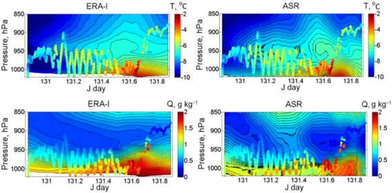
Flight 5 provided a series of 18 boundary layer profiles over a sea-ice-free region west of Svalbard. With the low wind speeds (< 5 m s−1), the 24 h balloon trajectory remained rel-atively close to the Svalbard coastline. Figures 8 and 9 com-pare the along-flight profiles of temperature, specific humid-ity and U and V winds measured by the CMET to ERA-I and ASR model reanalyses. From morning to afternoon increases in temperature and humidity at the surface are observed by the CMET and shown by both models. Note that the lowest ERA-I model level intersects the CMET sounding at low al-titudes (likely due to non-realistic surface topography), pre-venting model comparison, whereas this problem does not occur for ASR.
Overall there is good agreement between the reanalyses and CMET observations but some differences remain. Dur-ing the night of JD 130-131, ERA-I underestimates tem-perature compared to CMET. This is better reproduced by ASR up until midday on JD 131, although still underpre-dicted. Both models and the CMET nevertheless show rel-atively small variations in the temperature profiles at this time. Humidity is well reproduced by ASR during the JD 130-131 night and only slightly underestimated by ERA-I. On the morning of JD 131, ERA-I reproduces the observed enhanced humidity near the surface better than ASR. In ASR the vertical humidity transition is sharper than observed by the CMET and humidity is underestimated near the surface. Both ERA-I and ASR capture the observed increase in near-surface temperature and specific humidity up to the mid-afternoon. However, the CMET temperature increase is ei-ther stronger or earlier than in the models. These temperature and humidity enhancements are also spatio-temporally more localized for ASR than ERA-I. This leads to closer CMET agreement with ERA-I for mid-afternoon temperature but with ASR for humidity. Temperature is underestimated by both models at high altitudes in the evening of JD 131 whilst humidity is well reproduced (slightly overestimated by ERA-I).
Figure 8. Temperature and specific humidity measured during the CMET flight 5 soundings (filled circles) compared to 4-D interpolated (latitude, longitude, pressure, time) model data from ERA-I and ASR.
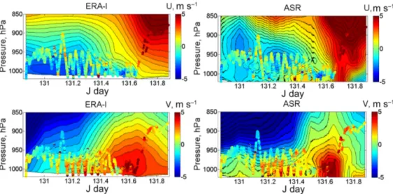
There are also differences in the U and V winds between ASR and ERA-I (Fig. 9). The CMET observes strong V wind shear on the morning of JD 131. This wind shear pattern is reproduced by ASR but is not captured by ERA-I. V winds become southerly (from direction) in mid-afternoon in both models, but are more localized in ASR, leading to better early afternoon model agreement, although ERA-I better repro-duces the persistence of southerly V winds to higher altitudes observed during the afternoon on JD 131. Westerly U winds are modelled and observed on the evening of JD 131. ERA-I shows high positive U winds at high altitudes only, whereas ASR shows high positive U winds at almost all levels.
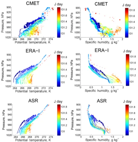
Closer inspection of the CMET temperature shows some signs of hysteresis in this flight with greater temperatures reached during ascents than descents. This is despite the fast time response of the (aspirated) thermistor. A possible ex-planation might be the heating of the balloon surface by the sun, raising the temperature of the air layer in direct contact with the balloon. This air layer could be transported over the sensor during ascent, but not descent profiles. Nevertheless, measurements made during descent only (> 0.1 m s−1 verti-cal descent speed) are consistent with the complete ascent– descent in potential temperature and specific humidity pro-files (Fig. 10). These propro-files show an overall increase (∼ 5– 6 K) in potential temperature observed close to the surface, which is reproduced by the models except for where ASR underpredicts the temperature rise (∼ 3–4 K) and ERA-I ex-hibits a potential temperature bias of ∼ −2 K. The observed trend in surface specific humidity is less clear but with an overall enhancement. ASR specific humidity is in agreement with the CMET on JD 131 morning but is underestimated by up to 0.5 g kg−1during the afternoon. ERA-I better captures the afternoon humidity maximum (and in early morning) but overestimates midday humidity by 0.5 g kg−1. The CMET
and model flight 5 profiles show less stable conditions than found for flight 4 (which showed an inversion layer). 3.4 CMET soundings in detail: decoupled flows and
wind field estimation
Further analysis of the observations from the CMET flight 5 on JD 131 enables consideration of local-scale patterns at higher resolution than the reanalyses. The observed profiles of potential temperature, specific humidity, wind speed and wind direction over ∼ 02–12.5 UTC (JD 131.08–131.52) are shown with interpolated data between the soundings to high-light temporally consistent features (Fig. 11). The soundings ranged from approximately 150 to 700 m during this period. As mentioned previously, specific humidity tends to increase during the flight, particularly in the lower and middle lev-els. However, beyond JD 131.40 (9.6 UTC) there is actually a decrease in humidity in the lowermost levels, with maxi-mum humidity in the sounding occurring at around 350 m al-titude. Concurrent to this there is also a small increase in po-tential temperature at low altitudes. The wind speed and di-rection plots indicate relatively calm conditions, with great-est wind speed in the lower levels from a general southerly direction. In contrast, at the top of the soundings the bal-loon encountered winds from a northerly direction, above 600 m. From JD 131.35 onwards, the observed winds became broadly southerly also at 600 m. However, a band of rather more west-south-westerly winds developed at mid-altitudes (∼ 450 m), and low-level winds became (east)-south-easterly from JD 131.4 onwards. This indicates that the balloon was not strictly sampling a uniform air mass during this pe-riod. Whilst previous studies have used CMETs to study La-grangian air mass trajectories (e.g. Voss et al., 2010), here the flight path is quasi-Lagrangian. As a consequence, the tem-perature and humidity trends observed along the flight path
Figure 9. U and V winds observed during the CMET flight 5 soundings (filled circles) compared to 4-D interpolated (latitude, longitude, pressure, time) model data from ERA-I and ASR.
cannot be wholly interpreted in Lagrangian terms (e.g. trac-ing of diurnal signature on a strac-ingle air parcel), rather they must also consider the Eularian perspective (e.g. advection of air masses with distinct properties into and out of the CMET flight path and their mixing).
The continuous series of CMET vertical profiles provide a more detailed overview of local-scale meteorology than is possible with traditional rawinsondes or constant-altitude free balloons. The CMET observations are consistent with the occurrence of a low-level flow that is decoupled from higher altitudes and – at least initially – an increase in sur-face humidity. The sursur-face winds may be influenced by low-level channel flows. An outflow commonly exits from nearby Kongsfjorden–Kongsvegen valley (e.g. Esau and Re-pina, 2012) but is hard to identify from the ground station in Ny Ålesund (south side of Kongsfjorden) given the rather low wind speeds during this period. Winds that originate over land are likely to be colder, with lower humidity than ma-rine air masses. Thus, the CMET observations of lower spe-cific humidity between JD 131.40 and 131.5 (9.6–12 UTC) might be explained by fumigation from or simply sampling of such a channel outflow. Alternatively, the CMET location near Kapp Mitra Peninsula at this time may indicate an even more local source of dry air impacting low levels. A final pos-sibility could be the overturning of air masses in the vertical, bringing less humid air with higher potential temperature to lower altitudes. At mid-levels (∼ 450 m) a relatively humid air layer persists, properties which suggest it has origins from the surface. It appears to be advected north-eastwards, po-tentially replenishing air over Svalbard to replace that which may be lost from the channel outflow.
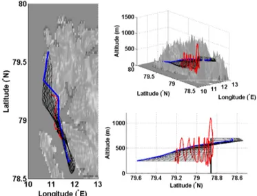
Wind fields are estimated from the CMET balloon 5 flight path for an 8 h period starting in the early morning of 11 May (JD 131) (Fig. 12). As per previous figures, the CMET bal-loon movement during the soundings has been used to
es-timate wind speed and direction. Here, wind trajectories are derived from the observed winds at 50 m altitude in-tervals for each up or down profile. The trajectory vectors (of length proportional to the wind speed × time elapsed be-tween soundings) are placed end-to-end to estimate the wind field, shown in Fig. 12 (grey mesh), alongside the CMET flight (red). This approximate technique assumes horizon-tally uniform flow in the vicinity of the balloon and computed trajectories. The lowermost layer exhibited the greatest wind speed, thus has the longest (and least certain) trajectory, ap-proximately double that of the balloon during the same pe-riod. The uppermost layer flows southwards before revers-ing direction, approximately returnrevers-ing to its initial position at 600 m altitude. The middle layer trajectory is quite simi-lar to that of the overall CMET balloon flight, but is trans-ported initially somewhat more westwards and later some-what more eastwards, due to the ESE winds experienced in the late morning (see Fig. 11). It is worth noting that this final direction mirrors findings from two of the other CMET balloons, which have flight paths out of Kongsfjor-den deviating to the north-east into the nearby KrossfjorKongsfjor-den (Fig. 1). These balloon-based trajectories provide insight into the complex local dynamics of low-altitude circulation influ-enced by complex terrain. Furthermore, the trajectories and profile data can be computed and displayed in near-real time to inform the real-time in-flight decisions on CMET altitude control (e.g. to track specific layers or events of meteorolog-ical interest).
3.5 Discussion: ASR and ERA-I model reanalyses in comparison to CMET
Both reanalyses showed good general agreement with the CMET flights, finding more stable conditions for flight 4 (over sea ice) than flight 5 (coastal). For flight 4, ASR showed
Figure 10. Profiles of potential temperature and specific humidity during flight 5 as observed by the CMET balloon and according to the 4-D interpolated ERA-I and ASR model outputs. CMET measurements made during descents only (> 0.1 m s−1vertical descent speed) are shown as filled circles and full data sets are shown as open circles.
a better capability than ERA-I to reproduce a temperature in-version observed over sea ice. ASR and ERA-I broadly re-produced the enhanced humidity near the sea ice surface but showed some discrepancies with the CMET in the vertical-spatial distributions. For flight 5, ASR better reproduced ob-served wind shear near to the Svalbard coast. Both models exhibit increasing specific humidity and temperature in the near-surface atmosphere from morning to afternoon on JD 131, in agreement with the trend observed. However, com-pared to the CMET the surface temperature and humidity enhancements were underpredicted by ASR. ERA-I under-estimated ABL temperature. Whilst increasing humidity and temperature over the daytime might be expected based on the diurnal cycle, Sect. 3.4 highlights the quasi-Lagrangian nature of flight 5 that also requires consideration of air mass advection and mixing. Figure 13 presents ERA-I (regional-scale) and ASR (local-(regional-scale) patterns for surface 2 m tem-perature and humidity for the duration of JD 131, alongside the CMET 5 flight path. A zone of warm and humid air ini-tially to the south-west of Svalbard advects northwards and eastwards. This likely exerted a significant influence on the observed and modelled along-flight surface trends. The ASR also clearly shows local diurnal influences on surface
me-teorology, particularly on 2 m temperature over the elevated topography east of the flight.
The temperature and humidity increases along flight 5 are temporally and spatially broader for ERA-I than for ASR (Fig. 8). This may to some degree reflect model diffusion on the larger ERA-I grid size (∼ 80 km compared to 15 km for ASR). The poorer ERA-I resolution of Svalbard topog-raphy will also affect simulated meteorology in this coastal area, where there may be local mixing, e.g. between marine-and lmarine-and-influenced air masses. A major contributing fac-tor to ASR performance in capturing observed wind shear (flight 5) and temperature inversion (flight 4) is likely the higher vertical model resolution of ASR compared to ERA-I, with ASR having about double the number of model levels than ERA-I at > 800 hPa, see Methods for descriptions. This improves the representation of the shallow polar ABL with its distinct layers. Noting that higher-resolution models that better capture spatial patterns can nevertheless lead to worse agreement with observations due to slight spatial shifts (Wes-selen et al., 2014), we choose not to reduce the ERA-I, ASR and CMET comparison to standard metrics (e.g. a correlation coefficient) here. The representations of Arctic air–sea–ice interaction and parameterization of turbulence fluxes in the
Figure 11. Potential temperature, specific humidity, wind speed and wind direction determined from the CMET balloon observations (131.08 to 131.52 JD, equivalent to ∼ 02 to 12.5 UTC on 11 May) of flight 5 during a series of automated soundings between 150 and 700 m altitude. Data between the balloon soundings has been interpolated.
Figure 12. Wind field calculated from the CMET balloon flight 5. Air parcel trajectories are calculated over an 8 h period for each 50 m altitude layer according to the winds observed by the CMET soundings. The red line shows the actual balloon track, the black vertical line shows the initialization of the calculation and the de-rived air parcel trajectories (wind field grid) are shown in grey. The blue line shows the final locations after 8 h.
boundary layer schemes will also influence the model outputs (e.g. Mölders and Kramm, 2010), but they are difficult to as-sess from this study. In future, this insight could be provided by campaigns in which multiple CMET balloons are sequen-tially colaunched to horizontally and vertically and probe an atmospheric region, combined with model sensitivity simu-lations.
4 Conclusions
Five Controlled Meteorological (CMET) balloons were launched from Ny-Ålesund, Svalbard on 5–12 May 2011, to measure in situ the meteorological conditions (humidity, temperature, winds, pressure) in the surrounding Arctic re-gion. Repeated soundings were performed along the CMET flights that probed the Arctic atmospheric boundary layer. The CMET data are analysed in comparison to model out-put from the ERA-Interim and Arctic System Reanalyses.
CMETs are a novel balloon technology capable of multi-day flights in the troposphere and performing in-flight sound-ings on command. Five CMET balloons were launched in May 2011. Balloons 1 and 2 had only short flights whilst bal-loon 3 made multi-day flights to the north but did not perform any soundings. Flights 4 and 5 made repeated soundings that profiled the ABL. CMET balloon 4 made two soundings of the boundary layer over sea ice to the east of Svalbard. De-spite good performance this flight needed to be terminated to avoid encroaching on Russian territory. CMET balloon 5 was placed in an automated soundings mode and made a suite of 18 continuous soundings along the north-west coast of Sval-bard, during a 24 h flight. To our knowledge, this was the first automated sounding sequence made by a free balloon.
This study focuses on the two flights that performed re-peated profiling of the boundary layer. Overall both observa-tions and models identify the ABL as more stable for flight 4 (over sea ice) than flight 5 (coastal). To the east of Svalbard (flight 4), the observed temperature and humidity increases towards the surface are generally well reproduced by ERA-I and ASR. The CMET observed a temperature inversion over sea ice which was reproduced by ASR but was not captured by ERA-I. ASR and ERA-I broadly reproduced the enhanced humidity near the sea ice surface but showed some discrep-ancies with the CMET in the vertical-spatial distributions. The CMET flight 5 along the north-west coast of Svalbard
Figure 13. Surface 2 m temperature and specific humidity over JD 131 according to ERA-I (upper) and ASR (lower). ERA-I outputs are shown on the regional scale at 6-hourly intervals whilst ASR outputs are shown on a local scale at 3-hourly intervals. The CMET flight 5 trajectory up to each time point is illustrated as a white line.
observed increases in near-surface humidity and temperature and strong wind shear. Detailed analysis of the CMET data identifies a low-level flow and provides an estimate of local wind fields. The wind shear was captured by ASR but not ERA-I. Both model reanalyses find increasing surface spe-cific humidity and temperature from morning to afternoon on JD 131. The enhancements are more spatio-temporally localized in ASR than ERA-I. The temperature enhancement was underpredicted by ASR whilst ERA-I exhibits a nega-tive temperature bias on JD 131. The higher vertical and hor-izontal resolution of the ASR captures features (temperature inversion in flight 4, wind shear in flight 5) that are not de-scribed by ERA-I. However, there are other aspects of the model–observation comparison that are in better agreement for ERA-I than ASR. This might be due to the different
rep-resentations of processes in the model and could be investi-gated in future by deploying a suite of CMET balloons over a region combined with model sensitivity studies.
In summary, CMET balloons provide a novel techno-logical means to profile the remote Arctic over multi-day flights, including the capacity to perform continuous au-tomated soundings into the atmospheric boundary layer. CMETs are thus highly complementary to other Arctic obser-vational strategies including fixed station, free and tethered balloons, meteorological masts and RPAS/UAVs (drones). Whilst RPAS/UAVs offer full 3-D spatial control for obtain-ing the meteorological observations, their investigation zone is generally limited to tens of kilometres based on both range and regulatory restrictions. CMET flights provide a relatively low-cost approach to observing the boundary layer at greater
distances from the launch site (e.g. tens to hundreds of kilo-metres), from tropospheric altitudes potentially all the way down to the surface, and more remotely from the distur-bances of Svalbard topography. CMETs can provide new in situ data sets for for quasi-Lagrangian and long-range trans-port and process studies.
5 Data availability
The CMET balloon data analysed in this study can be visual-ized online at http://www.science.smith.edu/cmet/flight.html and accessed by contacting the CMET balloon principal in-vestigator: Paul Voss at Smith College (pvoss@smith.edu). Two external model data sets were used in this work and are referenced in the text. ERA-Interim (ERA-I) model reanal-ysis data are available from http://apps.ecmwf.int/ (Dee et al., 2011). Arctic System Reanalysis (ASR) data v1 and soon v2 are available from http://rda.ucar.edu/ (Bromwich et al., 2016).
Acknowledgements. This research was sponsored by the Research Council of Norway and the Svalbard Science Forum. We are very grateful to the joint French–German Arctic Research Base AWIPEV in Ny-Ålesund for logistical support and Anniken C. Mentzoni for fieldwork assistance. Paul B. Voss also acknowledges Smith College for support. Tjarda J. Roberts acknowledges NSINK, an Arctic Field Grant, CRAICC, and the VOLTAIRE LABEX (VOLatils-Terre Atmosphère Interactions – Ressources et Environnement) ANR-10-LABX-100-01 (2011–20) for funding. This study occurred at the end of the Coordinated Investigation of the Climate-Cryosphere Interactions (CICCI) initiative. We are extremely grateful to the ASR team for providing model-level ASRv2 reanalysis data in advance of public distribution. We thank Chi-Fan Shih for help in accessing the ASR files and David Bromwich for useful comments on the manuscript.
Edited by: S. M. Noe
Reviewed by: three anonymous referees
References
Andreas, E. L., Guest, P. S, Persson, P. O. G., Fairall, C. W., Horst, T. W., Moritz, R. E., and Semmer, S. R.: Near-surface water va-por over polar sea ice is always near ice saturation, J. Geophys. Res.-Oceans, 107, C10, doi:10.1029/2000JC000411, 2002. Bromwich D. H., Hines K. M., and Bai L.-S.:
Develop-ment and testing of polar weather research and forecast-ing model: 2. Arctic Ocean, J. Geophys. Res., 114, D08122, doi:10.1029/2008JD010300, 2009.
Bromwich, D. H., Wilson, A. B., Bai, L., Moore, G. W. K., and Bauer, P.: A comparison of the regional Arctic System Reanaly-sis and the global ERA-Interim ReanalyReanaly-sis for the Arctic, Q. J. Roy. Meteor. Soc., 142, 644–658, doi:10.1002/qj.2527, 2016. Dee, D. P., Uppala, S. M., Simmons, A. J., Berrisford, P., Poli,
P., Kobayashi, S., Andrae, U., Balmaseda, M. A., Balsamo, G.,
Bauer, P., and Bechtold, P.: The ERA-Interim reanalysis: Con-figuration and performance of the data assimilation system, Q. J. Roy. Meteor. Soc., 137, 553–597, doi:10.1002/qj.828, 2011. Esau, I. and Repina, I.: Wind Climate in Kongsfjorden,
Sval-bard, and Attribution of Leading Wind Driving Mechanisms through Turbulence-Resolving Simulations, Adv. Meteorol., 2012, 568454, doi:10.1155/2012/568454, 2012.
Hole L. R., Bello, A. P., Roberts, T. J., Voss, P. B., and Vihma, T.: Measurements by controlled meteorological bal-loons in coastal areas of Antarctica, Antarct. Sci., CJO2016, doi:10.1017/S0954102016000213, 2016.
Kilpeläinen, T., Vihma, T., and Olafsson, H.: Modelling of spatial variability and topographic effects over arctic fjords in svalbard, Tellus A, 63, 223–237, 2011.
Mäkiranta, E., Vihma, T., Sjöblom, A., and Tastula, E.-M.: Obser-vations and modelling of the atmospheric boundary layer over sea-ice in a svalbard fjord, Bound.-Lay. Meteorol., 140, 105–123, 2011.
Maturilli, M., Herber, A., and König-Langlo, G.: Climatology and time series of surface meteorology in Ny-Ålesund, Svalbard, Earth Syst. Sci. Data, 5, 155–163, doi:10.5194/essd-5-155-2013, 2013.
Mayer, S., Sandvik, A., Jonassen, M., and Reuder, J.: Atmospheric profiling with the UAS SUMO: a new perspective for the evalu-ation of fine-scale atmospheric models, Meteorol. Atmos. Phys., 116, 15–26, 2012a.
Mayer, S., Jonassen, M., Sandvik, A., and Reuder, J.: Profiling the arctic stable boundary layer in Advent Valley, Svalbard: Mea-surements and simulations, Bound.-Lay. Meteorol., 143, 507– 526, 2012b.
Mölders, N. and Kramm, G.: A case study on wintertime inversions in interior Alaska with WRF, Atmos. Res., 95, 314–332, 2010. Moore, G. W. K., Renfrew, I. A., Harden, B. E., and Nernild, S.
H.: The impact of resolution on the representation of south-east Greenland barrier winds and katabatic flows, Geophys. Res. Letts., 42, 3011–3018, doi:10.1002/2015GL063550, 2015. Moore, G. W. K., Bromwich, D. H., Wilson, A. B., Renfrew,
I., and Bai, L.: Arctic System Reanalysis improvements in topographically-forced winds near Greenland, Q. J. Roy. Meteor. Soc., 142, 2033–2045, doi:10.1002/qj.2798, 2016.
Persson, P. O. G., Fairall, C. W., Andreas, E. L., Guest, P. S., and Perovich, D. K.: Measurements near the atmospheric surface flux group tower at sheba: Near-surface conditions and surface energy budget, J. Geophys. Res., 107, 8045–8079, 2002.
Riddle, E. E., Voss, P. B., Stohl, A., Holcomb, D., Maczka, D., Washburn, K., and Talbot, R. W.: Trajectory model validation us-ing newly developed altitude-controlled balloons durus-ing the in-ternational consortium for atmospheric research on transport and transformations 2004 campaign, J. Geophys. Res., 111, D23S57, doi:10.1029/2006JD007456, 2006.
Rinke, A., Dethloff, K., Cassano, J., Christensen, J., Curry, J., Du, P., Girard, E., Haugen, J.-E., Jacob, D., Jones, C., Kltzow, M., Laprise, R., Lynch, A., Pfeifer, S., Serreze, M., Shaw, M., Tjern-strm, M., Wyser, K., and Agar, M.: Evaluation of an ensemble of Arctic regional climate models: spatiotemporal fields during the sheba year, Clim. Dynam., 26, 459–472, 2006.
Smedsrud, L. H., Esau, I., Ingvaldsen, R. B., Eldevik, T., Hau-gan, P. M., Li, C., Lien, V. S., Olsen, A., Omar, A. M., Ot-terå, O. H., and Risebrobakken, B.: The role of the Barents
Sea in the Arctic climate system, Rev. Geophys., 51, 415–449, doi:10.1002/rog.20017, 2013.
Stenmark, A., Hole, L. R., Voss, P., Reuder, J., and Jonassen, M. O.: The influence of nunataks on atmospheric bound-ary layer convection during summer in Dronning Maud Land, Antarctica, J. Geophys. Res. Atmos., 119, 6537–6548, doi:10.1002/2013JD021287, 2014.
Tjernström, M., Birch, C. E., Brooks, I. M., Shupe, M. D., Pers-son, P. O. G., Sedlar, J., Mauritsen, T., Leck, C., Paatero, J., Szczodrak, M., and Wheeler, C. R.: Meteorological conditions in the central Arctic summer during the Arctic Summer Cloud Ocean Study (ASCOS), Atmos. Chem. Phys., 12, 6863–6889, doi:10.5194/acp-12-6863-2012, 2012.
Vihma, T., Lüpkes, C., Hartmann, J., and Savijärvi, H.: Observa-tions and modelling of cold-air advection over Arctic sea ice in winter, Bound.-Lay. Meteorol., 117, 275–300, 2005.
Vihma, T., Pirazzini, R., Fer, I., Renfrew, I. A., Sedlar, J., Tjern-ström, M., Lüpkes, C., Nygård, T., Notz, D., Weiss, J., Marsan, D., Cheng, B., Birnbaum, G., Gerland, S., Chechin, D., and Gascard, J. C.: Advances in understanding and parameteriza-tion of small-scale physical processes in the marine Arctic cli-mate system: a review, Atmos. Chem. Phys., 14, 9403–9450, doi:10.5194/acp-14-9403-2014, 2014.
Voss, P. B., Zaveri, R. A., Flocke, F. M., Mao, H., Hartley, T. P., DeAmicis, P., Deonandan, I., Contreras-Jiménez, G., Martínez-Antonio, O., Figueroa Estrada, M., Greenberg, D., Campos, T. L., Weinheimer, A. J., Knapp, D. J., Montzka, D. D., Crounse, J. D., Wennberg, P. O., Apel, E., Madronich, S., and de Foy, B.: Long-range pollution transport during the MILAGRO-2006 cam-paign: a case study of a major Mexico City outflow event using free-floating altitude-controlled balloons, Atmos. Chem. Phys., 10, 7137–7159, doi:10.5194/acp-10-7137-2010, 2010.
Voss, P. B., Hole, L. R., Helbling, E., and Roberts, T. J:. Continu-ous in-situ soundings in the Arctic boundary layer: A new atmo-spheric measurement technique using controlled meteorological balloons, J. Intell. Robotic Syst., 70, 609, doi:10.1007/s10846-012-9758-6, 2012.
Wesslén, C., Tjernström, M., Bromwich, D. H., de Boer, G., Ek-man, A. M. L., Bai, L.-S., and Wang, S.-H.: The Arctic sum-mer atmosphere: an evaluation of reanalyses using ASCOS data, Atmos. Chem. Phys., 14, 2605–2624, doi:10.5194/acp-14-2605-2014, 2014.