A Correlation method to determine monthly cooling energy consumption in Canadian homes

Publisher’s version / Version de l'éditeur: Building Research Journal, 3, Fall 2, pp. 12-34, 1994

READ THESE TERMS AND CONDITIONS CAREFULLY BEFORE USING THIS WEBSITE.

https://nrc-publications.canada.ca/eng/copyright

Vous avez des questions? Nous pouvons vous aider. Pour communiquer directement avec un auteur, consultez la première page de la revue dans laquelle son article a été publié afin de trouver ses coordonnées. Si vous n’arrivez pas à les repérer, communiquez avec nous à PublicationsArchive-ArchivesPublications@nrc-cnrc.gc.ca.

Questions? Contact the NRC Publications Archive team at

PublicationsArchive-ArchivesPublications@nrc-cnrc.gc.ca. If you wish to email the authors directly, please see the first page of the publication for their contact information.

Archives des publications du CNRC

This publication could be one of several versions: author’s original, accepted manuscript or the publisher’s version. / La version de cette publication peut être l’une des suivantes : la version prépublication de l’auteur, la version acceptée du manuscrit ou la version de l’éditeur.

Access and use of this website and the material on it are subject to the Terms and Conditions set forth at

A Correlation method to determine monthly cooling energy

consumption in Canadian homes

Newsham, G. R.; Sander, D. M.; Moreau, A.

https://publications-cnrc.canada.ca/fra/droits

L’accès à ce site Web et l’utilisation de son contenu sont assujettis aux conditions présentées dans le site LISEZ CES CONDITIONS ATTENTIVEMENT AVANT D’UTILISER CE SITE WEB.

NRC Publications Record / Notice d'Archives des publications de CNRC: https://nrc-publications.canada.ca/eng/view/object/?id=307a5846-495f-4c3b-9b45-da80c41dcbdb https://publications-cnrc.canada.ca/fra/voir/objet/?id=307a5846-495f-4c3b-9b45-da80c41dcbdb

A Corre la t ion m e t hod t o de t e rm ine m ont hly c ooling e ne rgy

c onsum pt ion in Ca na dia n hom e s

N R C C - 3 7 9 0 1

N e w s h a m , G . R . ; S a n d e r , D . M . ; M o r e a u , A .

F a l l 1 9 9 4

A version of this document is published in / Une version de ce document se trouve dans:

Building Research Journal, 3, (2), Fall, pp. 12-34, 94

The material in this document is covered by the provisions of the Copyright Act, by Canadian laws, policies, regulations and international agreements. Such provisions serve to identify the information source and, in specific instances, to prohibit reproduction of materials without written permission. For more information visit http://laws.justice.gc.ca/en/showtdm/cs/C-42

Les renseignements dans ce document sont protégés par la Loi sur le droit d'auteur, par les lois, les politiques et les règlements du Canada et des accords internationaux. Ces dispositions permettent d'identifier la source de l'information et, dans certains cas, d'interdire la copie de documents sans permission écrite. Pour obtenir de plus amples renseignements : http://lois.justice.gc.ca/fr/showtdm/cs/C-42

A Correlation Method to Determine Monthly Sensible Cooling

Energy Consumption in Canadian Homes

Guy R. Newsham, Dan M. Sander, and Alain Moreau

ABSTRACT

Building on the development of a correlation method to determine seasonal residential cool-ing energy in Canada, we developed a similar correlation method to predict delivered sensible cooling energy on a monthly basis. Further, we investigated the effect of thermal mass and manual venting on the sensible cooling energy requirement. The predictions using the

monthly method were compared

to

those from an hourly simulation model and found

to

be sat-isfactory given the method's simplicity. Mean differences, over all climates and building pa-rameters considered, were 6.5 percent in the light mass, no manual venting case. An exam-ple calculation using the method is presented, and the method's limitations are discussed.

Guy R. Newsham is a Research Associate, Institute for Research in Construction, National Research Council of Canada, Ottawa, Ontario. Dan M. Sander is a Senior Research Officer, Institute for Research in Construction, National Research Council of Canada, Ottawa, Ontario. Alain Moreau is a Research Engineer, LTEE,

Hydro-Quebec, Shawinigan Quebec.

INTRODUCTION

Many Canadian utilities have supported pro-grams

to

encourage the adoption of energy effi-cient electrical appliances in the home.

Efficient appliances will not only affect the en-ergy consumption of the home directly, through ·_heir own reduced electricity consumption, but also indirectly, through their reduced heat out-:JUt (internal gains). Reduced internal gains mean an increased load on the heating system, and a decreased load on the cooling system; any assessment of the total energy impact of ef-ficient appliances must account for these ther-mal effects. It is only recently, with an

explosion of residential air conditioning owner-ship (Ontario Hydro 1990), that cooling effects have become potentially significant in Canada. This perhaps explains the lack of any existing simple method

to

accurately determine the im-pact of internal gains on residential cooling en-ergy consumption.

In a previous paper (Newsham, Sander and Moreau 1993) we described the development of a correlation method

to

determine seasonal residential cooling energy consumption in Can-ada. Although this seasonal correlation was relatively accurate, it did assume that resi-dences were cooled throughout the five month summer period from May

to

September. For many Canadian homes the cooling season is shorter than this, and, therefore, we extended the method to determine sensible cooling for

in-dividual summer months. This paper describes the extension of the method

to

monthly calcula-tions.

METHODS AND PROCEDURES

We used the EASI hourly simulation model to calculate the sensible cooling requirements from which we derived the correlations. EASI employs the ASHRAE Transfer Function Method (ASHRAE 1993), and was originally de-veloped by Public Works Canada. The hourly simulation runs were exactly the same as those described in Newsham, Sander and Moreau (1993). However, for the monthly correlations, the cooling energy requirement was summed monthly rather than seasonally.

In summary, the modeled house was offloor area CAr) 160m2, external wall area CAw) 184

m2 and volume (V) 604m3• Cooling setpoint for

the summer months was 24 °C, and the maxi-mum ventilation rate, with windows open due to manual venting, was 0.2 m3s·1• The following

parameters were varied between runs: • Internal gains per unit floor area

(including occupants): 0 to 12.5 W/m2, constant schedule.

• Glazing (fraction of wall area glazed x shading coefficient): 0 to 0.5. • Heat loss factor, HLF ([sum

ofu-value x area, for walls, roofs, and windows, and including infiltration] I Ar): 0 to 2.89 W/m2_·°C

• Venting strategy: windows shut (non-vented) or manually openable windows (vented).

• Thermal mass per unit floor area: 60 kJ/m2·°C (light) or 150 kJ/m2_·°C

(medium).

The vented strategy attempted to account for residents' efforts to cool a house through in-creased ventilation before resorting to mechani-cal cooling. We modeled this action in the following way: If the cooling load could be met by increased ventilation then infiltration was considered to be increased to the rate necessary to satisfy the cooling setpoint (up to the given maximum air flow rate); if the maximum air flow rate was inadequate to meet the cooling load, then the infiltration rate remained at the minimum rate (i.e., the windows were consid-ered shut) and mechanical cooling took over.

There are many strategies that occupants can adopt with respect to air conditioner use (New-sham, Sander and Moreau 1993), and the strat-egy described above is just one of them.

Nevertheless, our assumptions represent an oc-cupant gaining reasonable maximum ventila-tive free cooling, and, thus, form a lower boundary to the cooling energy requirements.

A total of 1848 parameter combinations for each of eight Canadian cities were considered. Monthly cooling requirements were simply the sum of the calculated hourly cooling require-ments of that month. Only the months May to September were considered; we assume that, ir-respective of the parameter values, mechanical cooling would not be engaged in Canadian resi-dences outside of these months.

HOURLY COOUNG CORRELATION

Non-vented Case, Low Mass

The correlation equation for monthly sensi-ble cooling energy in the non-vented case is of the same form as that previously derived for seasonal cooling energy (Newsham, Sander and Moreau 1993), except that coefficients appropri-ate for a monthly rather than a seasonal calcu-lation must be used:

Cr!Gtot = e1 + f1 · [ GtotiGs ] + ez · [ ln( 11Gtot) ]

+ fz · [ Gtot!Gs] · [ln(l!Gtot )] + e3 • [ln (Gtot!Lt)]

+ {3 · [ GtotiGs] · [ln (Gtot!Lt)] + e4 · [ln(l!Gtot)] · [ln (GtotiLt)]

+ {4 · [ Gtot!Gs] · [ln (1/Gtot )] · [ln (Gtot!Lt)]

(1)

where

Cr = sensible cooling energy for month per unit floor area, kWhlm2;

Gi =total of internal gains for month per unit floor area, kWh/m2;

G8

=

total of solar gains for month per unit floor area, kWhlm2

;

Gtot = G8 + Gi, kWh/m

2 ;

Lt

=maximum contribution transmission loss can make to reducing the cooling load for month per unit floor area, kWhlm2_{; and} ｾＮ＠ fi are climate dependent coefficients.

Cr/Gtot is, therefore, the fraction of solar plus internal gains which must be removed by the

Table 1. Correlation coefficients for Ottawa for the low mass case MAY JUN Hm 744 720 kt 7.40 3.99 e1 0.0248 0.2198 &.z -0.1944 -0.1546 es 0.2741 0.2040 e4 0.0500 0.0359 fl 0.0562 -0.1377 f2 0.0725 0.0030 fs 0.1420 0.1552 f4 0.0253 0.0292 VInl VIn2 vms VIn4

mechanical cooling system. Note that Cr is the delivered sensible cooling energy; to convert Cr to the billed energy one must divide by the ap-propriate COP of the air conditioner. Table 1

gives values for the coefficients ｾ＠ and

fi

which were determined for Ottawa. Appendix A de-scribes a method for determining these coeffi-cients from monthly climate statistics.

Parameter Gi depends only on the occupancy and the internal gains. In developing the corre-lation we assumed a constant internal gain schedule; therefore:

(2)

where

Hm

=

hours in the month;

I = average total internal gains (including occu-pants) for month, W; and

JUL AUG SEP

744 744 720 2.73 2.87 6.75 0.9065 0.5558 0.1596 -0.0147 -0.0862 -0.1669 -0.0431 0.0830 0.2256 -0.0141 0.0114 0.0402 -0.3022 -0.2018 0.0084 -0.0560 -0.0200 0.0554 0.1388 0.1408 0.1505 0.0243 0.0249 0.0278

Applies to All Months

0.8743 -0.4678 -0.0099 0.0024

Parameters G8 , and Lt are building and

cli-mate dependent. G8 is described by the follow-ing equation:

G8

=

0.32 · <Agn ·Sen· VSN +A88 • SCs · VSS

+Age· See· VSE +Agw ·Sew· VSW

· ( Hm/24 )I Ar (3)

where

ｾ＠

=

area of glass facing orientation i (where, i=n is north; i=s is south; i=e is east; and i=w is west);

sci

= shading coefficient of windows facing ori-entation i;

VSS

=

mean daily solar radiation on south verti-cal, for the month, MJ/m2;

VSN = mean daily solar radiation on north verti-cal, for the month, MJ/m2;

VSW = mean daily solar radiation on west verti-cal, for the month, MJ/m2; and

VSE = mean daily solar radiation on east verti-cal, for the month, MJ/m2•

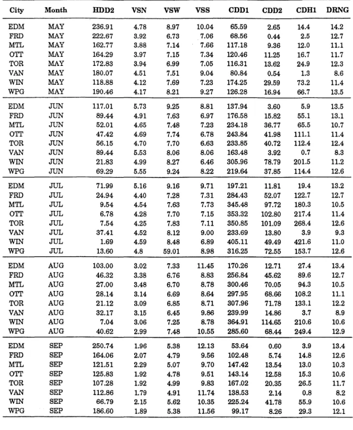
VSS, VSN, and VSW can be found in Table 2, which shows all relevant monthly climate data for the 8 cities studied; note, for this climate data, VSE

=

VSW.

Parameter Lt is described by the following equation:

Lt=kt ·HLF (4)

where HLF is the heat loss factor, given by:

HLF'= (Aw · Uw +Ar · Ur+Ag · Ug+

0.329 · V · ACH )/

Ar

(5)

where

Aw

= total area of opaque walls, m2;

Uw =average U-value of opaque walls, W/m2-°C;

Ar:

=total area of roof, m2;

Ur =average U-value of roof, W/m2-°C;

Ag =total area of windows, m2;

Ug =average U-value of windows, W/m2-°C;

V =volume, m3;

ACH = average infiltration, acJh; and kt is a climate dependent coefficient.

Values ofkt for Ottawa are given in Table 1. Appendix B describes a method for determining the coefficient kt from monthly climate statis-tics.

Manual Window Opening (Vented Case), Low Mass

The monthly sensible cooling energy require-ment in the vented case is expressed in terms of the appropriate monthly cooling energy re-quirement for the non-vented case. Plotting the cooling energy consumption from the hourly model for the vented case versus that for the non-vented case for various months and

pa-rameter combinations (examples are shown in

Figure 1) suggested the following relationship:

Cf(vent) ( Lt, Gs, Gi )

=

Cf(non-vent ( Lt, Gs, 0 ) - vm1- vm2 · Gt-vma · Gs · Gi-um4 · Lt · Gi

(6)

where

vm11 vm2, vm3, and vm4 are climate dependent

coefficients.

Values ofvmi for Ottawa are given in Table 1. Appendix C describes a method for de-termining these coefficients from monthly cli-mate statistics.

Cf(vent) is also bound by the condition:

0 < Cf(ven() < ｃｦＨｮｯｮＭｬｬ･ｮｾ＠ (7)

Effect of Mass

The above results were all derived for a low mass house construction (60 kJ/ m2·°C). This construction is representative of the majority of residences built in Canada. However, there are residences with higher internal mass, and we repeated the derivation process for a medium mass case (150 kJ/ m2·°C) to determine the ef-fect of mass on cooling energy. Example build-ing constructions conformbuild-ing to the above two mass types are shown in Table 3.

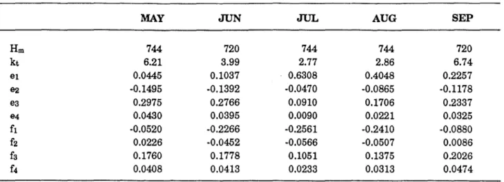
The form of the correlation equations in the medium mass case is exactly the same as for the low mass case; however, the correlation co-efficients are changed. Table 4 gives values of

co-･ｦｦｩ｣ｩ･ｮｴｳｾＮ＠ fil kt, and vmi for the medium mass case for Ottawa. Appendix A describes a

method for determining the coefficients ei and

fi

from monthly climate statistics. Appendices B and C describe a method for determining the co-efficients

kt

and vmi, respectively, from

monthly climate statistics.

We also assume that the following condition applies( the assumption appears to be con-firmed by our analysis):

Table 2. Climate parameters for 8 Canadian cities, monthly. EDM =Edmonton; FRD =Fredericton; Mn =Montreal; OTT= OHawa; TOR= Toronto; VAN= Vancouver; WIN= Windsor; WPG =Winnipeg

City

EDM

FRD

MTL

OTr

TOR

VAN

WIN WPG

EDM

FRD

MTL

OTr

TOR

VAN

WIN WPG

EDM

FRD

MTL

OTr

TOR

VAN

WIN WPG

EDM

FRD

MTL

OTr

TOR

VAN

WIN WPG

EDM

FRD

MTL

OTr

TOR

VAN

WIN WPG Month

MAY

MAY MAY

MAY

MAY

MAY

MAY

MAY JUN JUN JUN JUN JUN JUN JUN JUN JUL JUL JUL JUL JUL JUL JUL JUL AUG AUG AUG AUG AUG AUG AUG AUG SEP SEP

SEP

SEP

SEP

SEP

SEP

SEP

HDD2 236.91 222.67 162.77 164.29 172.83 180.07 118.88 190.46 117.01 89.44 52.01 47.42 56.15 89.44 21.83 69.29 71.99 24.94 9.54 6.78 7.54 37.41 1.69 13.60 103.00 46.32 27.00 28.14 21.12 32.17 7.04 40.62 250.74 164.06 121.51 125.83 107.28 112.86 66.79 186.60

VSN

4.78 3.92 3.88 3.97 3.94 4.51 4.12 4.17 5.73 4.91 4.65 4.69 4.70 5.53 4.99 5.55 5.16 4.40 4.54 4.28 4.25 4.52 4.59 4.8 3.02 3.38 3.48 3.14 3.09 3.15 3.06 2.99 1.96 2.07 2.29 1.92 1.92 1.79 2.15 1.89

vsw

8.97 6.73 7.14 7.15 6.99 7.51 7.69 8.21 9.25 7.63 7.48 7.74 7.70 8.06 8.27 9.24 9.16 7.28 7.63 7.70 7.83 8.12 8.48 59.01 7.33 6.76 6.70 6.69 6.85 6.45 7.25 7.48 5.38 4.79 5.07 4.78 4.99 4.91 5.62 5.38

vss

10.04 7.06 7.66 7.34 7.05 9.04 7.23 9.27 8.81 6.97 7.23 6.78 6.63 8.06 6.46 8.22 9.71 7.31 7.73 7.15 7.11 9.00 6.89 8.98 11.45 8.83 8.78 8.64 8.71 9.86 8.78 10.55 12.13 9.56 9.70 9.51 9.83 11.74 10.35 11.56 CDD1 65.59 68.56 117.18 120.46 116.31 80.84 174.25 126.28 137.94 176.58 234.18 243.84 233.85 163.48 305.96 219.64 197.21 284.43 345.48 353.32 350.85 233.69 405.11 316.25 170.26 256.84 300.46 297.95 307.96 239.99 364.91 285.60 53.64 102.48 147.42 143.14 167.02 138.53 225.24 99.17 CDD2 2.65 0.44 9.36 11.25 13.62 0.54 29.59 16.94 3.60 15.82 36.77 41.98 40.72 3.92 78.79 37.85 11.81 52.07 97.72 102.80 101.09 13.80 49.49 72.55 12.71 45.62 70.05 68.66 71.78 14.86 114.65 68.44 0.60 5.74 13.54 12.58 20.35 2.14 41.78 8.26 CDH1 DRNG 14.4 14.2 2.5 12.7 12.0 11.1 16.7 11.7 24.9 12.3 1.3 8.6 73.2 11.4 66.7 13.5 5.9 13.5 55.1 13.1 65.5 10.7 111.1 11.4 112.4 12.4 0.7 8.3 201.5 11.2 114.4 12.6 19.4 13.2 122.7 12.7 180.3 10.5 217.4 11.4 268.4 12.6 3.9 9.3 421.6 11.0 153.7 12.6 27.4 13.4 89.6 12.7 94.3 10.5 108.2 11.1 133.1 12.2 3.7 8.9 210.6 10.6 249.4 12.9 3.9 13.4 14.8 12.6 13.0 10.3 15.3 10.6 26.5 11.7 0.8 8.2 55.9 10.6 29.3 12.1

s::

ｾ＠

-o

ｾ＠II >

Toronto

Septerrber, HLF

=

0

Toronto

_{July, HLF}

=

₀

8000 _eooo Gi Gl 8000 SeWg 4000 2000 ₂₀₀₀ 4000 6000 8000 10000 _{4000 6CXXl 8000 IIXX)O} Non-vented, kWh _{Non-vented, kWh} (a) _(b)

Toronto

Juty, ScWg

=

0.5 8000 s:: ｾ＠ 6000

-o

_II

c

₄₀₀₀ II > 2000 Non-vented, kWh (c)

Figure 1. The relationship between sensible cooling energy requirement in the vented and non-¥ented cases, for various months and

pa-rameter combinctlons (W9

=

fraction of well crec glozed). In panels (c) end (b) there ere six sets of curves, one for each of six differ·

en! values of the parameter SeW

a.

The eleven points within each set show eleven different values of G;. In panel (c) there ere two sets

of curves, one for each of two ditterent values of U. The eleven points within each set show eleven different values of G;.

light 60

medium 150

Tobie 3. House constructions end associated thermal mess

Construction

wood frame construction 13 mm gypsum interior imish on walls and ceilings, carpets over wooden floors.

as above, but 50 mm gypsum interior finish on walls, and 25 mm gypsum interior finish on ceiling

Table 4. Correlation coefficients for OHawa for the medium mass case MAY JUN

Hm

744 720 kt 6.21 3.99 e1 0.0445 0.1037 ｾ＠ -0.1495 -0.1392 ea 0.2975 0.2766 e4 0.0430 0.0395 fl -0.0520 -0.2266 fz 0.0226 -0.0452 fa 0.1760 0.1778 f4 0.0408 0.0413 Yml vmz vma Ym4

DISCUSSION: GOODNESS OF FIT

Figure 2 shows, for the low mass, non-vented case, the monthly sensible cooling energy con-sumption calculated using the correlation vs. EASI monthly cooling energy consumption, for Ottawa. In a large majority of cases, the differ-ences are less than 10 percent. Newsham and Sander (1994) contains similar plots for all eight cities studied, for both the vented and non-vented cases. Table 5 _{summarizes the mean}

percentage differences for all eight cities for both the vented and non-vented cases. Mean percentage differences are less than 10 percent in three-quarters of the cases. However, the percentage differences in May, and in some cases September, are higher; one might expect this since the absolute cooling requirements in these two months tend to be small. Hence, in May and September, the mean percentage dif-ferences can be misleading and tend to overesti-mate the importance of small absolute

differences in small cooling energy require-ments.

JUL AUG SEP

744 744 720 2.77 2.86 6.74 0.6308 0.4048 0.2257 -0.0470 -0.0865 -0.1178 0.0910 0.1706 0.2337 0.0090 0.0221 0.0325 -0.2561 -0.2410 -0.0880 -0.0566 -0.0507 0.0086 0.1051 0.1375 0.2026 0.0233 0.0313 0.0474

Applies To All Months

1.2146 -0.4707 -0.0102 -0.0045

Table 6 shows the mean percentage differ-ences between the seasonal cooling energy re-quirement calculated by the hourly model and that calculated from a sum of the appropriate monthly correlations. By comparing Table 5

with the results reported in Newsham, Sander and Moreau (1993) one can see that, in most cases, a sum of monthly correlations is slightly worse at predicting the seasonal sensible cool-ing energy consumption than the seasonal cor-relation described by Newsham, Sander and Moreau (1993). However, summing the monthly correlations to obtain a seasonal cool-ing energy requirement is by no means unac-ceptable because mean percentage differences are lower than 8 percent in all cases.

Figure 3 shows, in the non-vented case, the ratio of cooling energy requirement in the me-dium and low mass cases versus the cooling en-ergy requirement in the low mass case, for sensible cooling calculated using the hourly model and the correlation. Only the values cov-ering a range of typical house parameters are shown, and only plots for July and September

8000 2000 2000

Ottawa - no vent

May 2000 4000 6000 EASI,kWh

Ottawa - no vent

July 8000 10%

ｾ＠

1

8 10% .•.• ·•···••···••···· 10% 2000 4000 6000 8000 EASI,kWh 8000 2000

Ottawa - no vent

September 2000 4000 6000 EASI,kWh 8000 6000 4000 2000 8000 2000 10% 8000

Ottawa - no vent

June 2000 4000 6000 EASI,kWh

Ottawa - no vent

August 2000 4000 6000 EASI,kWh 10% .. ···· 10% 8000 8000

Figure 2. Monthly sensible cooling energy consumption for Ottowa calculated using the correlation versus that calculated using the hourly model, for all building parameter variations, for the non-vented case, for the light moss house. Ten percent difference levels are indicated.

Table 5 . .'Aean percentage differences between the monthly sensible cooling energy consumption calculated by an hourly model and

that calculated by the correlation, For all building parameter variations; low mass house.

City Month Mean Differences, percent non-vented vented Edmonton MAY 11.4 12.3 Fredericton MAY 14.1 19.5 Montreal MAY 5.8 26.5 Ottawa MAY 11.9 15.8 Toronto MAY 9.3 12.2 Vancouver MAY 9.9 11.8 Windsor MAY 10.4 19.2 Winnipeg MAY 10.3 10.9 Edmonton JUN 4.6 8.2 Fredericton JUN 2.0 4.9 Montreal JUN 3.5 5.6 Ottawa JUN 3.2 6.9 Toronto JUN 2.5 4.6 Vancouver JUN 7.1 8.3 Windsor JUN 4.7 4.5 Winnipeg JUN 4.7 5.9 Edmonton

JUL

3.9 7.0 Fredericton JUL 7.9 7.2 Montreal JUL 6.0 7.2 Ottawa JUL 10.0 5.8 Toronto JUL 4.3 6.2 Vancouver JUL 3.0 7.3 Windsor JUL 7.7 6.3 Winnipeg JUL 3.5 7.9 Edmonton

AUG

4.9 11.1 Fredericton

AUG

3.0 7.8 Montreal

AUG

7.1 4.6 Ottawa

AUG

6.0 5.5 Toronto

AUG

4.0 5.4 Vancouver

AUG

3.4 10.0 Windsor

AUG

8.3 5.9 Winnipeg

AUG

5.2 5.6 Edmonton SEP 10.8 13.8 Fredericton SEP 7.8 11.5 Montreal SEP 4.3 5.4 Ottawa SEP 6.4 9.8 Toronto SEP 3.7 5.3 Vancouver SEP 14.3 11.2 Windsor SEP 3.3 3.3 Winnipeg SEP 7.2 8.3

Table 6. Mean percentage differences between the seasonal sensible cooling energy consumption calculated by an hourly model and

that calculated using the sum of the monthly correlations, For all building parameter variations, For a low moss house.

City Fredericton Montreal Ottawa Toronto Windsor Winnipeg Edmonton Vancouver

Ottawa -

July

HLF (0.5-1.5); ScWg (0.1-0.4); Gi (2.5-1 0.0) ｾ＠ 1 . 1 . - - - , ｾ＠ 1. UJ ;;;- 0. gJ 0.8 E 0.7 3:: .Q 0.6 -;;; 0.5 (/)

e

o.4 E 0.3 .2 02 "0 Ql 0.1 E ｯＮｯＫＭＭＮＭＭＭＭＮＭＭＭＮＭＭＭＬＭＭＭＬＭＭＮＮＮＬＮＭＭＮＬＭＭＭ｟｟｟ＬＮＭＭＭＭＮＭｾ＠ 1000 2000 3000 4000 5000 6000 7000 8000 9000 1 0000

low mass, kWh(EASJ)

Ottawa - September

HLF (0.5-1.5); ScWg {0.1-0.4); Gi (2.5-1 0.0) ｾ＠ 1 . 1 . - - - , ｾ＠ 1.0--og. Ａ｢ｾ＠

ｾｯＺＸ＠

, , , -3:: 0.7 '0 .Q 0.6 -(/) 0.5 Cl Cl (/)

e

o.4 Cl E 0.3 .2 0.2 "0 ｾ＠ 0.1 ｏＮｏｩＺＭｾｲＺＭＺＭＭＺＺＺＺ｣ＺＭＺＭＭＺＺＭＺＭｲＺＺＭＺＭＭＭＭｲＭＭＬＭＭＮＮＮＬＮＭＭＮＮＭＭＭＬＮＭＭＭＭＮＭｾＮ＠ ｾ＠ Ｌｾ＠ 1000 2000 3000 4000 5000 6000 7000 8000 9000 1 v NO

low mass, kWh(EASJ)

Mean Differences, percent non-vented vented 3.6 4.4 3.6 4.3 4.7 4.0 2.5 4.0 5.4 3.9 3.1 5.2 4.9 7.4 4.2 6.1

Ottawa -

July

HLF (0.5-1.5); ScWg (0.1-0.4); Gi (2.5-1 0.0)

w

1.1 8 1. -; 0. gJ 0.8 E 3:: 0.7 .Q 0.6 -;;; 0.5 (/)

e

o.4 E 0.3 ｾ＠ 0.2 ｾ＠ 0.1 Jib§;' m: T a ｏＮｏｩＺＭｾｲＺＭＺＭＭＺＺＺＺ｣ＺＭＺＭＭＺＭＺ｣ＺＭＺＺＭＭＭＺＭ］ＺＭＭＺＺ］ＭＺＭＭＺＭＺｲ］Ｍ］Ｚ｣ＺＺＭＭＭＺＭ］Ｇ］Ｇ］ＢＧＭＺＭＺｯＭＺＭＺＭＭＺＭ _{1 000 2000 3000 4000 . 5000 6000 7000 8000 9000 1 0}

low mass, kWh(correl)

Ottawa - September

HLF {0.5-1.5); ScWg {0.1-0.4); Gi (2.5-10.0) = 1 . 1 , -{g ＸＱＮｾ＠

;o.

F

-gJ 0.8 Cl E 3:: 0.7 § .Q 0.6 -;;; 0.5 (/)

e

o.4 E 0.3 .2 02 "0 ｾ＠ 0.1 o.ot---:-::1ooo=--=2000=:--=3000=--::4000=--=5000=:--=so::r::oo:-:-=7ooo:>:-:-_8 __ 000.,----9000--,--1 c low mass, kWh (correl)

Figure 3. The ratio of the sensible cooling energy requirement in the medium moss house to that in the low moss house vs. the sensible cooling energy requirement in the low moss house, calculated using both the hourly model and the correlation, for various parameter

in Ottawa are shown as examples. The effect of mass is small for all but the very lowest cooling loads, reducing sensible cooling load by less than 20 percent in most cases. The correlation performs adequately, reproducing the trends exhibited by the hourly model output. Since the mass effect is small, calculating the cooling en-ergy consumption for thermal masses within the range 60 to 150 kJ/ m2·°C can be done by linear interpolation.

Table 7 _{shows the mean percentage}

differ-ences for all eight cities for both the vented and non-vented cases, in the medium mass case. In general, the differences for the medium mass correlation are a little higher than those for the low mass case. Nevertheless, mean percentage differences are less than 10 percent in most cases, though the percentage differences par-ticularly in May and September are higher. However, to reiterate, the mean percentage dif-ferences can be misleading and tend to overesti-mate the importance of small absolute

differences in small cooling energy require-ments. Newsham and Sander (1994) contains plots similar to Figure 2 for all eight cities stud-ied, for both the vented and non-vented cases, for a medium mass house.

LIMITATIONS

The applicability of the simple monthly cal-culation method presented here is limited by some of the assumptions used in deriving the correlations:

• We assumed a constant internal gain schedule for simplicity. During the development of complementary seasonal cooling correlations (New-sham, Sander and Moreau 1993) we compared correlations developed from a more realistic schedule with those developed from a constant schedule and found no significant difference. However, the correla-tions described in this paper might prove more unreliable for internal · gain schedules very different from constant. Remember, we expected the method

to

be applied

to

large populations ofhouses in which the mean internal gain schedule would lack dramatic peakso

• Heat loss to the basement was not considered. In the majority of Cana-dian houses the basement is not di-rectly conditioned, and therefore in summer would be at a lower tem-perature than the rest of the house. Thus, there is the possibility of free cooling to the basement. However, in most cases, due to basement air stratification and poor coupling be-tween the basement and the rest of the house, the effect of summertime heat loss to the basement would be small. If consideration of basement heat loss is required, it could be cal-culated separately and included in the correlation as a reduction in in-ternal gains. Basement heat loss can be treated in this manner be-cause it will be close to constant over a 24 hour period, which matches our assumption for the in-ternal gains proflle.

• A single zone model was assumed for the house. Therefore, it applies only to the case in which the entire house (excepting the basment) is conditioned to the same tempera-ture, and there is good mixing of the indoor air.

• Attic temperature was not simu-lated by the hourly model from which the correlation was derived; heat transfer through the roof was modeled as though the attic was at outdoor temperature. This results in an underestimate of cooling re-quirements. In Canada, where it is

normal for the ceiling to be highly insulated and the attic to be well ventilated, this is not a serious inac-curacy. However, it may be signifi-cant when this is not the case. • Glazing was assumed to be equally

distributed in the four cardinal di-rections. Again, this assumption was made with the expectation that the method would be applied to large populations ofhouses, where the mean glazing distribution would be close to equal. However, we an-ticipate that the method can be

Table 7. Mean percentage differences between the monthly sensible cooling energy consumption calculated by an hourly model and that calculated by the correlation, for all building parameter variations; medium mass house.

City Month Mean Differences, percent non-vented vented Edmonton MAY 19.4 22.1 Fredericton MAY 30.1 37.4 Montreal MAY 10.2 15.7 Ottawa MAY 23.4 32.0 Toronto MAY 17.4 28.5 Vancouver MAY 23.8 26.4 Windsor MAY 22.5 38.6 Winnipeg MAY 17.2 24.7 Edmonton JUN 6.9 12.9 Fredericton JUN 2.5 6.6 Montreal JUN 5.4 7.8 Ottawa JUN 5.2 9.8 Toronto JUN 3.6 7.1 Vancouver JUN 17.0 17.7 Windsor JUN 6.4 6.4 Winnipeg JUN 6.2 10.7 Edmonton JUL 8.0 10.9 Fredericton JUL 6.6 9.9 Montreal JUL 5.7 10.3 Ottawa JUL 4.3 7.3 Toronto JUL 4.3 10.8 Vancouver JUL 4.8 10.5 Windsor JUL 1.4 6.0 Winnipeg JUL 5.3 12.6 Edmonton AUG 5.9 14.9 Fredericton AUG 8.1 8.6 Montreal AUG 4.8 6.1 Ottawa AUG 4.7 7.0 Toronto AUG 4.7 8.0 Vancouver AUG 5.9 13.1 Windsor AUG 4.4 8.0 Winnipeg AUG 4.3 9.4 Edmonton SEP 20.3 26.4 Fredericton SEP 20.5 22.0 Montreal SEP 10.1 8.7 Ottawa SEP 20.8 27.7 Toronto SEP 5.9 9.4 Vancouver SEP 17.8 25.1 Windsor SEP 4.7 4.8 Winnipeg SEP 12.4 15.0

used with other glazing distribu-tions provided that the resulting so-lar gain profile is not very different from that produced by an equal dis-tribution (see example below). • Only two thermal masses were

stud-ied. The effect of mass was found to be small, so a linear interpolation is probably adequate for masses in be-tween these two.

• The correlation calculates sensible cooling load only and not latent loads; thus, the correlation will al-ways underestimate the total load. The ratio of total load to sensible load will vary hourly depending, in part, on the system characteristics. Since EASI does not model system performance we did not address la-tent loads in this study.

• The correlations were developed for the climates of only eight Canadian

cities. At this point the method should only be used for the cities and climate data noted in this pa-per. Future work could expand the applicability of the method to other climates.

• The equations give the cooling re-quired by the space (delivered en-ergy); they do not include the cooling equipment efficiency charac-teristics. They are intended to be used with an assumed coefficient of performance for the air conditioning unit.

APPUCA TION - AN EXAMPLE

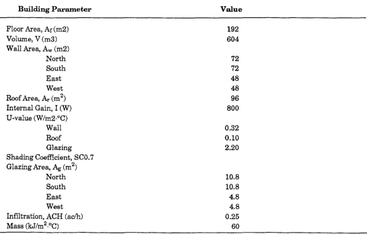
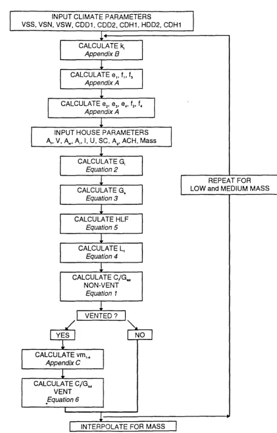
The following is a step-by-step example of ap-plying the method to calculate the sensible cool-ing energy for a typical scool-ingle-family detached house in Ottawa in July, for the non-vented case. Table 8 shows the house input parame-ters. Figure 4 is a flow diagram outlining the

Table 8. Building parameters for a typical single-family detached house Building Parameter Floor Area, Ar (m2) Volume, V (m3) Wall Area, Aw (m2) North South East West Roof Area, Ar (m2) Internal Gain, I (W) U-value (W/m2·°C) Wall Roof Glazing Shading Coefficient, SCO. 7 Glazing Area, .Ag (m2)

North South East West Infiltration, ACH (aclh) Mass (kJ/m2·°C) Value 192 604 72 72 48 48 96 800 0.32 0.10 2.20 10.8 10.8 4.8 4.8 0.25 60

procedure to be followed when calculating the cooling energy consumption using the monthly correlation. From Equation 2: Gi

= (

744 · 800 )/( 192 · 1000)

=

3.10 From Equation 3: G8

=

0.32 · ( 0.15 · 72 · 0.7 · 4.28 + 0.15 · 72 · 0.7 . 7.15 + 0.1· 48. 0.7. 7.7 + 0.1· 48. 0.7. 7.7) . ( 744/24 )/192

=

7.13 and therefore: Gtot

=

3.10 + 7.13

=

10.23 From Equation 5: HLF

=

(208.8 · 0.32 + 96 · 0.1 + 31.2 · 2.2 + 0.329 . 604 . 0.25 )/192

=

1.01 From Equation 4, and using the relevant value ofkt from Table 2:

Lt

=

2.73 · 1.01

=

2.77

Now, from Equation 1, and using the rele-vant values of ei and

fi

from Table 2:

Cr!Gtot = 0.9065- 0.3022 · [ 10.23/7.13] - 0.0147 · [ln ( 1/10.23)] - 0.0560 · [10.23/7.13] · [ln/10.23)] - 0.0431 . [ln ( 10.23/2.77)] + 0.1388 · [ 10.23/7.13] · [ln (10.23/2.77)] -0.0141· [ln ( 1/10.23)] · [ln ( 10.23/2.77)] + 0.0243 · [ 10.23/7.13] · [ln ( 1/10.23)] · [ln ( 10.23/2.77)] = 0.834

In other words, 83.4 percent of the total so-lar and internal gains in July need to be re-moved by the cooling system.

Therefore, the delivered sensible cooling en-ergy per unit floor area is:

2

Cr= 0.834 · 10.23

=

8.53 kWhlm

and the total delivered sensible cooling energy is:

8.53 · 192 = 1638 kWh

(assuming a COP of 3, the billed cooling energy is 1638/3 = 546 kWh).

The EASI hourly model predicts a July deliv-ered sensible cooling energy for the same build-ing of 1462 kWh, for a difference between the correlation and EASI of 12 percent, which is ac-ceptable. Repeating this process for the five months of the cooling season (May to Septem-ber), and summing the predictions for each of the months yields a predicted seasonal deliv-ered cooling energy consumption from the corre-lation of 5756 kWh. EASI predicts a seasonal value of 5727 kWh, remarkably close to the value predicted by the correlation. Note that the glazing in the example house was far from equally distributed in each of the four cardinal directions; equal distribution of glazing was the assumption on which the correlation was based. The level of agreement in the predic-tions between the correlation and EASI sug-gests that the method can indeed be

successfully applied to other glazing distribu-tions.

We compared the predictions of the correla-tion and EASI for seven variacorrela-tions on the exam-ple house shown in Table 8. Table 9 details the variations, and Figures 5 and 6 show the com-parisons for July and for the cooling season, re-spectively. Although the correlation

consistently overestimates the sensible cooling in July (when compared to EASI), the differ-ences are acceptable for a simple method such as this one. The only difference greater than 12 percent is for variation F, where the glazing dis-tribution is very unequal. The seasonal com-parison shows all differences less than 9 percent. The greatest difference occurs for vari-ation H. In this case the majority of the glazing faces east and west rather than north and south, as in the initial example house (vari-ation A). Whereas the hourly solar gain distri-bution for variation A will be similar to that given by an equal glazing distribution (noon peak), variation H will likely yield a distribu-tion with peaks in morning and afternoon, sig-nificantly different from the equal glazing

INPUT CLIMATE PARAMETERS

I

VSS, VSN, VSW, CDD1, CDD2, CDH1, HDD2, CDH1

I

I

CALCULATE 1\ Appendix 8 CALCULATE e,. f,. f, Appendix A

CALCULATE e₂, e,, e,, f₂, f,

Appendix A

I

INPUT HOUSE PARAMETERS A,. V,

A..

A,, I, U, SC. A •. ACH, Mass

CALCULATE G; Equation2

l

CALCULATE G, Equation 3

!

CALCULATE HLF Equation 5

l

CALCULATE L, Equation 4

l

CALCULATE C/G.,. NON-VENT Equation 1

l

/I

I

YES

I

!

VENTED? CALCULATE vm, .. AppendixC CALCULATE C/Gtot VENT .Equation 6

l·

]""'

I

NO

I

I

I

INTERPOLATE FOR MASS

I

I

REPEAT FOR

I

LOW and MEDIUM MASS

Table 9. Variations on the example house described in Table 8 Variation Description A B

c

D E F G H

House, as described in Table 8 Internal Gains, I

=

1200 W Internal Gains, I

=

400 W Mass= 150 kJ/m2.°C

Infiltrtion Rate, ACH

=

0.75 aclh

Agn = 7.2 m2, Ags= 25.2 m2, Age= 9.6 m2, Agw = 4.8 m2

Aw (all walls)= 60m2; Ag (all walls)= 7.8 m2 Rotate Variation A 90

°

' [ ] ' 18.0 _{correl j} r -

.

,

ｾ＠ 115 _! 5.8

i

r

...

12.0

n

3.4 11.5 11.3

!

f I I i : i i I 0 E G building variation

Figure 5. Comparison of the sensible cooling energy for July

predicted by the correlation and the hourly model; for 8 build-ing parameter variations in Ottawa.

distribution assumption on which the correla-tion was based.

CONCLUSIONS

A simple correlation equation to determine monthly residential sensible cooling energy con-sumption in Canada has been developed. It al-lows the quick determination of the change in residential cooling energy consumption with changes in internal gain, envelope U-value,

12

'cJl

7.2 carrel !

•

9.6 ｾ＠ 2.6

..

" 0.5 u u

...

i

_i

i _! I I I I I I I ;

I

I

i I I I i 2.4 C 0 E G building vanation

Figure 6. Comparison of the sensible cooling energy for the 5

month cooling season predicted by the correlation and the hourly model; for 8 building parameter variations in Ottawa.

glazing area, shading coefficient, and thermal mass.

As the correlation was developed for a Cana-dian house with equal glazing on all facades and thermal masses of 60 and 150 kJflC-m2

,

the correlation will be most accurate when ap-plied to houses of this construction and form. However, other constructions and forms can be accommodated with appropriate care.

Considering its simplicity, the correlation is relatively accurate. The mean percentage

differ-ence compared to the output of an hourly model, over a wide range of building parame-ters and climates, ranged from 6.5 percent in a low mass house with no manual venting, to 14.9 percent in a medium mass house where manual venting was considered.

REFERENCES

ASHRAE. 1993. American Society of Heating, Refrig-erating and Air-Conditioning Engineers Hand· book of Fundamentals, Chapter 26. Atlanta, ASHRAE.

Newsham, G.R. and D.M. Sander. 1994. Develop-ment of a simple method to determine the frac-tion of internal gains that contribute to an increase in cooling load in air conditioned Cana-dian homes. IRC Internal Report No. 658, Na-tional Research Council Canada, Ottawa. Newsham, G.R., D.M. Sander, and A. Moreau. 1993.

A correlation equation to determine residential cooling energy consumption in Canada. Building Research Journal, 2 (1), 39-52.

Ontario Hydro. 1990. Residential appliance survey: report no. MR 91-61. Ontario Hydro, Toronto, Canada.

Tse-Chih, A. 1991. Project to prepare climatic design information for ASHRAE standard 90.1-1989 and ASHRAE handbook. Environment Canada,

APPENDIX A

Determination of Coefficients ej and fi from Climate Statistics;

Non-Vented Case.

As with the seasonal correlation equations described in Newsham, Sander and Moreau (1993), the climate coefficients of Equation 1 ap-propriate for a monthly calculation were found

to be linearly related. For the low mass, non-vented case: e2 = -0.199457 + 0.203834 · e1 es = 0.28305 - 0.359833 · e1 e4 = 0.051848- 0.072774 · e1 {2 = 0.052369 + 0.358601· {1 {4 = -0.017041 + 0.298164. {3

These relationships are illustrated in New-sham and Sander (1994).

(A-1) (A-2)

(A-3)

(A-4)

(A-5)

Therefore, climate dependence for only three of the coefficients (e_1, f1, fa), need be derived. e11

flo fa can be correlated to monthly climate pa-rameters:

e1,{1,{3, =ao+a1· VS+a2 · VSS +aa · CDDl

+ U4 . CDD2 + U5 . CDH1 + U6 . DRNG (A-6)

where

VS

=

VSS + VSN + 0.5 (VSE + VSW);

CDD1 =monthly Cooling Degree Days (base 10

oc);

CDD2 = monthly Cooling Degree Days (base 18.3 °C);

CDH1 = monthly Cooling Degree Hours (base

26.7 °C);

DRNG =mean Daily temperature RaNGe for the month (°C); and

ao

to

as

are coefficients given in Table A-1.

Figures in Newsham and Sander (1994) illus-trate the relationship between elo flo fa derived

from the individual regressions for each loca-tion, and the ell flo f3 derived from the climate

correlations of Equation A-6, for all eight cities and five months.

It is important to note that the above correla-tion to climate was derived only for the eight cities and specific climate data noted in this pa-per. While future work considering more cities promises a universal climate correlation, we would not at present recommend its use beyond the climate data noted in this paper.

In the medium mass case:

e2 =-0.15728 + 0.17475 · e1 (A-7)

ea = 0.313123- 0.35211 · e1 (A-8)

e4 = 0.045556 - 0.05797 · e1 (A-9)

{2 = 0.042722 + 0.387759. fl (A-10)

{ 4 = -0.00275 + 0.247787 · fs (A-ll)

These relationships are illustrated in New-sham and Sander (1994).

Again:

e1,{1,{3 =ao +a1· VS +a2 · VSS +as· CDD1

+ a4 · CDD2 +as · CDH1 + a6 · DRNG

(A-12)

The coefficients

ao

to a6 for the medium

mass case are given in Table .A·2.

Figures in Newsham and Sander (1994) illus-trate the relationship between ell fll f3 derived

from the individual regressions for each loca-tion, and the ell fll f3 derived from the climate

correlations of Equation A-12, for all eight cit-ies and five months.

Table A-1. Coefficients necessary to determine e1, f1, fJ From the dim ate correlations; low mass case

MAY

JUN JUL AUG SEP

et ao -1.39541 13.15385 1.78257 6.402761 -0.70549 at 0.296447 -0.97771 1.492269 -0.13341 0.150486 a2 -0.66077 2.062468 -3.7051 -0.06433 -0.17138 8.3 0.012591 -0.04664 0.004475 -0.01051 -1.4e-05 li4 -0.0839 0.060232 -0.00354 0.014375 0.01261 li5 0.010402 0.021536 -0.01011 0.002957 -0.00561 86 0.004698 -0.14801 -0.17113 -0.09032 -0.00146 ft ao 0.293972 -0.9157 -0.7205 -1.65304 0.958032 at -0.06345 0.157542 -0.23948 0.032763 -0.20992 a2 0.127003 -0.41656 0.634356 0.014746 0.26714 8.3 -0.00317 0.003431 -0.00058 0.001893 -0.00222 li4 0.015237 -0.00415 -0.00155 -0.00198 0.008331 li5 -0.00134 -0.00369 0.002573 -0.00096 -0.00072 86 0.01996 0.028396 0.023578 0.035538 0.012869 fa ao 0.306439 -0.2966 0.19518 -0.44132 -0.21076 at 0.000715 0.028915 -0.02661 0.033069 0.070312 a2 0.003143 -0.03287 0.062417 -0.03012 -0.09102 8.3 -0.00053 0.001417 -0.00032 0.001043 0.001604 li4 0.003678 -0.00228 0.000651 -0.00197 -0.00971

li5 -0.0003 -0.00027 -9.9e-05 -5.4e-05 0.002505

Table A-2. Coefficients necessary to determine e1, fJ, fJ From the dimote correlations; medium moss case

MAY JUN JUL AUG SEP

e1 ao 1.525311 3.90778 0.774683 5.846196 0.676635 a1 0.364147 -0.90353 1.394302 -0.03328 0.047836 a2 -0.80666 1.862019 -3.38367 -0.22363 -0.07224 a;J 0.014173 -0.04935 0.005036 -0.0102 -0.0025 8..4 -0.09772 0.064825 -0.00663 0.010229 0.018419 8.5 0.012713 0.020568 -0.00863 0.002956 -0.00528 116 -0.00405 -0.17965 -0.16185 -0.07906 -0.03141 fl ao 0.196194 -0.62047 -0.25574 -0.84882 0.160245 a1 0.04247 0.108252 -0.09499 -0.01719 -0.17782 a2 0.078267 -0.29899 0.250371 0.079434 0.255015 a;J -0.00428 0.00157 -0.00084 1.24e-05 -0.00086 8..4 0.015275 -0.00126 0.001049 0.002758 0.003546 8.5 -0.00049 -0.00267 0.000878 -0.00083 -0.00067 116 0.026722 0.02704 0.002168 0.012216 0.028077 fa ao 0.568372 -0.91094 -0.07323 -0.73152 0.808987 a1 -0.05366 0.103803 -0.05073 0.052554 0.025018 a2 0.114884 -0.20423 0.150215 -0.05242 -0.06664 a;J -0.00151 0.003896 -0.00037 0.001477 -0.00022 8..4 0.012402 -0.00509 -0.00015 -0.00323 -0.00467 8.5 -0.00158 -0.00196 0.000402 -0.00018 0.002953 116 -0.01512 -0.00342 0.011707 0.013734 -0.03142

APPENDIX B

Determination of Coefficient kt from Climate Statistics; Non-Vented Case.

kt is the value that the term {[Cr (U-value,

G8 , Gi) -Ct<O, G8 , Gi)] I HLF) tends to over the

given period, calculated by the hourly model, as

G8 and Gi tend to their upper limits. The term {[Cr <U-value, Ga, Gi) -

Cc

CO, Ga, Gi)]

I

HLF} is the contribution of the transmission loss in re-ducing the cooling load, its value as Ga and Gi

tend to their upper limits indicates the trans-mission loss's maximum contribution. After try-ing many parameter combinations, kt was found to be accurately correlated to monthly cli-mate parameters:

kt

=

ao + a1 · HDD2 + a2 · VS + aa · VSS +a4 -CDD1+a5 ·CDD2+a6 ·DRNG where

(B-1)

HDD2

=

monthly Heating Degree Days (base 18.3 °C); and

coefficients Bo to ｾ＠ are given in Table B·l.

Figures in Newsham and Sander (1994) com-pare kt derived from the hourly model and kt derived from the climate correlation of Equa-tion B-1, for all eight locaEqua-tions, and all five months.

In the medium mass case:

kt=ao +a1· HDD2 +a2 · VS +as· VSS + U4 • CDDl + a5 · CDD2 + a6 · DRNG

(B-2)

The coefficients

ao

to

aa

in the medium mass case are given in Table 8·2.

Table B-1. Coefficients necessary to determine kt from the dimate correlations; low mass case

MAY JUN JUL AUG SEP

ao 3.036601 332.5413 ·25924.2 -402.18 17.22645 at 0.023506 -1.31738 100.5315 1.456179 0.024881 a2 -0.08896 0.209174 1.333325 1.708286 -2.8231 aa 0.265454 0.654212 -1.81128 -2.03485 3.532247 a4 -0.00905 -1.37387 100.7769 1.533788 -0.00769 as 0.084042 1.394898 -100.879 -1.60275 0.053997 as 0.028848 0.157998 -0.2942 0.288399 -0.09609

Table B-2. Coefficients necessary to determine kt from the dimate correlations; medium mass case

MAY JUN JUL AUG SEP

ao 2.07735 335.0168 -25976.2 -404.218 17.28512 at 0.022945 -1.32752 100.7332 1.463149 0.02451 a2 -0.10594 0.203216 1.344585 1.720076 -2.81628 aa 0.297673 0.674291 -1.83491 -2.04599 3.525458 a4 ·0.01021 -1.38409 100.979 1.541272 -0.00818 as 0.086852 1.405381 -101.081 -1.61041 0.054387 as 0.032787 0.161463 -0.29585 0.289251 -0.09582

Figures in Newsham and Sander (1994) com-pare kt derived from the hourly model and kt derived from the climate correlation of Equa-tion B-2, for all eight locaEqua-tions, and all five months.

Only for the month of May is there a signifi-cant change in the value ofkt with mass. This may be due to the influence of heating in early May.

APPENDIX C

Determination of Coefficients VlDi from Climate Statistics.

We found that a good result could be

achieved with the simplification that vml> vm_2, vm3, and vm4 are correlated to appropriate

an-nua,l rather than monthly, climate parameters. Such that:

vm1-4 = bo + b1 · VSa +in · VSSa + ba · CDDla + b4 ·CD !:£a+ b5 · CDHla + bs · DRNGa (C-1)

where

VSSa= mean daily solar radiation on south verti-cal, MJ/m2;

VSNa= mean daily solar radiation on north verti-cal, MJ/m2;

VSW a= mean daily solar radiation on west verti-cal, MJ/m2;

VSEa= mean daily solar radiation on east verti-cal, MJ/m2;

CDD18= annual Cooling Degree Days (base 10 oc);

CDD2a= annual Cooling Degree Days (base 18.3

oc);

CDH1a= annual Cooling Degree Hours (base 26.7 °C);

DRNGa= mean Daily temperature RaNGe for July (°C); and

bo to

hs

are coefficients given in Table C·l.

Appropriate annual climate parameters may be found in Table C·2 (from Tsi-Chih 1991). Note, for this climate data, VSEa

=

VSWa .

Table C-1. Coefficients necessary to determine vm1..t from the dimate correlations; low mass case

bo hi h2 ba b4 b5 bs

Yml -3.88719 0.123579 0.018138 0.001987 -0.000581 -0.002386 0.098205

Vffi2 -3.19051 0.120353 -0.116823 0.001521 -0.003760 -0.000323 0.065662

vma 0.026307 -0.000425 -0.000092 -0.000030 0.000079 -8e-07 -0.000795 Ym4 0.187758 -0.006591 0.005453 -0.000096 0.000183 0.000035 -0.004898

Table C-2. Climate parameters appropriate for the seasonal correlation of Yml-4 for 8 Canadian cities.

City HDD2a VSa VSSa CDDla CDD2a CDHla DRNGa

Fredericton 4840 18.21 9.20 928 124 319 12.7 Montreal 4615 17.65 8.67 1201 226 315 10.6 Ottawa 4758 18.27 9.13 1164 212 407 11.4 Toronto 4218 17.37 8.34 1201 224 510 12.5 Windsor 3687 18.82 8.86 1535 371 781 10.9 Winnipeg 5965 21.11 10.99 1000 169 479 12.5 Edmonton 5938 21.06 10.97 592 27 88 13.1 Vancouver 3112 17.12 8.25 859 30 8 9.1

Figures in Newsham and Sander (1994) illus-trate the relationship between vm14 derived

from the individual regressions for each loca-tion, and vm14 derived from the climate

correla-tions of Equation C-1, for all eight cities. For the medium mass case:

vm 1-4 = bo + b1 · VSa + l)2 · VSSa + ba · CDDia.

+ b4 · CDD?.a + b5 · CDHia. + b6 · DRNGa (C-2)

The coefficients b0 to b6 for the medium

mass case are given in Table C·3.

Figures in Newsham and Sander (1994) illus-trate the relationship between vm14 derived

from the individual regressions for each loca-tion, and vm1_4 derived from the climate

correla-tions of Equation C-2, for all eight cities.

Tobie C-3. Coefficients necessary to determine vm 14 from the dimote correlations; medium moss case

bo bt _h:! ba h4 h5 bs

Vlnl -17.42494 0.671511 -0.468594 0.009234 -0.015321 -0.003958 0.417536 Vln2 -3.93434 0.140368 ·0.132056 0.001870 ·0.003925 ·0.000653 0.090006

vma 0.0224138 0.000737 ·0.001803 -0.000032 0.000061 0.0000070 -0.000713