Understanding Type Ia supernovae through their $U$-band spectra

January 8, 2018

Understanding Type Ia supernovae through their U-band spectra

J. Nordin

, G. Aldering

, P. Antilogus

, C. Aragon

, S. Bailey

, C. Baltay

, K. Barbary

, S. Bongard

, K. Boone

,

V. Brinnel

, C. Buton

, M. Childress

, N. Chotard

, Y. Copin

, S. Dixon

, P. Fagrelius

, U. Feindt

, D. Fouchez

,

E. Gangler

, B. Hayden

, W. Hillebrandt

, A. Kim

, M. Kowalski

, D. Kuesters

, P.-F. Leget,

, S. Lombardo

,

Q. Lin

, R. Pain

, E. Pecontal

, R. Pereira

, S. Perlmutter

, D. Rabinowitz

, M. Rigault

, K. Runge

, D. Rubin

,

C. Saunders

, G. Smadja

, C. Sofiatti

, N. Suzuki

, S. Taubenberger

, C. Tao

, and R. C. Thomas

The Nearby Supernova Factory

1 _{Institut fur Physik, Humboldt-Universitat zu Berlin, Newtonstr. 15, 12489 Berlin}

2 _{Physics Division, Lawrence Berkeley National Laboratory, 1 Cyclotron Road, Berkeley, CA, 94720}

3 _{Laboratoire de Physique Nucléaire et des Hautes Énergies, Université Pierre et Marie Curie Paris 6, Université Paris Diderot Paris}

7, CNRS-IN2P3, 4 place Jussieu, 75252 Paris Cedex 05, France

4 _{Department of Physics, Yale University, New Haven, CT, 06250-8121}

5 _{Berkeley Center for Cosmological Physics, University of California Berkeley, Berkeley, CA, 94720}

6 _{Department of Physics, University of California Berkeley, 366 LeConte Hall MC 7300, Berkeley, CA, 94720-7300}

7 _{Université de Lyon, F-69622, Lyon, France ; Université de Lyon 1, Villeurbanne ; CNRS/IN2P3, Institut de Physique Nucléaire}

de Lyon.

8 _{Department of Physics and Astronomy, University of Southampton, Southampton, Hampshire, SO17 1BJ, UK} 9 _{The Oskar Klein Centre, Department of Physics, AlbaNova, Stockholm University, SE-106 91 Stockholm, Sweden} 10 _{Aix Marseille Université, CNRS/IN2P3, CPPM UMR 7346, 13288, Marseille, France}

11 _{Clermont Université, Université Blaise Pascal, CNRS/IN2P3, Laboratoire de Physique Corpusculaire, BP 10448, F-63000}

Clermont-Ferrand, France

12 _{Max-Planck Institut für Astrophysik, Karl-Schwarzschild-Str. 1, 85748 Garching, Germany} 13 _{Deutsches Elektronen-Synchrotron, D-15735 Zeuthen, Germany}

14 _{Tsinghua Center for Astrophysics, Tsinghua University, Beijing 100084, China}

15 _{Centre de Recherche Astronomique de Lyon, Université Lyon 1, 9 Avenue Charles André, 69561 Saint Genis Laval Cedex, France} 16 _{Space Telescope Science Institute, 3700 San Martin Drive, Baltimore, MD 21218}

17 _{European Southern Observatory, Karl-Schwarzschild-Str. 2, 85748 Garching, Germany}

18 _{Computational Cosmology Center, Computational Research Division, Lawrence Berkeley National Laboratory, 1 Cyclotron Road}

MS 50B-4206, Berkeley, CA, 94720

19 _{Kavli Institute for the Physics and Mathematics of the Universe, University of Tokyo, 5-1-5 Kashiwanoha, Kashiwa, Chiba,}

277-8583, Japan Received ; accepted

ABSTRACT

Context. Observations of Type Ia supernovae (SNe Ia) can be used to derive accurate cosmological distances through empirical standardization techniques. Despite this success neither the progenitors of SNe Ia nor the explosion process are fully understood. The U-band region has been less well observed for nearby SNe, due to technical challenges, but is the most readily accessible band for high-redshift SNe.

Aims.Using spectrophotometry from the Nearby Supernova Factory, we study the origin and extent of U-band spectroscopic variations in SNe Ia and explore consequences for their standardization and the potential for providing new insights into the explosion process. Methods.We divide the U-band spectrum into four wavelength regions λ(uNi), λ(uTi), λ(uSi) and λ(uCa). Two of these span the Ca h&k λλ 3934, 3969 complex. We employ spectral synthesis using SYNAPPS to associate the two bluer regions with Ni/Co and Ti. Results.(1) The flux of the uTi feature is an extremely sensitive temperature/luminosity indicator, standardizing the SN peak lumi-nosity to 0.116 ± 0.011 mag RMS. A traditional SALT2.4 fit on the same sample yields a 0.135 mag RMS. Standardization using uTi also reduces the difference in corrected magnitude between SNe originating from different host galaxy environments. (2) Early U-band spectra can be used to probe the Ni+Co distribution in the ejecta, thus offering a rare window into the source of lightcurve power. (3) The uCa flux further improves standardization, yielding a 0.086 ± 0.010 mag RMS without the need to include an additional intrinsic dispersion to reach χ2_{/dof ∼ 1. This reduction in RMS is partially driven by an improved standardization of Shallow Silicon}

and 91T-like SNe.

Key words. Cosmology : observations, supernovae – general, dark energy

1. Introduction

Type Ia supernovae (SNe Ia) are standardizable candles, and measuring their relative distances first led to the discovery of

Article number, page 1 of 19

dark energy (Riess et al. 1998; Perlmutter et al. 1999). Their ori-gin as thermonuclear explosions of CO WDs is well accepted, as is their importance as producers of heavy elements in the Uni-verse (e.g. Maoz et al. 2014). It is further accepted that the light curve is powered by the decay of56_{Ni, which has a half-life of}

∼ 6 days for the dominant decay channel to Co. However, the progenitor system configuration and the path to detonation is still not understood. While a small sample of nearby SNe Ia now have tight limits on companions set by the lack of interaction or non-detection of hydrogen (Leonard 2007; Bloom et al. 2012; Maguire et al. 2016), some SNe do show signs of H interaction (Hamuy et al. 2003; Aldering et al. 2006; Dilday et al. 2012) and theoretical explanations of the observed diversity prefer multiple explosion channels (Sim et al. 2013; Maeda & Terada 2016).

Current lightcurve-based empirical SN Ia standardization methods yield a ∼ 0.1 mag intrinsic dispersion (after accounting for measurement uncertainties), interpreted as a random scatter in magnitude and/or color (Betoule et al. 2014; Scolnic et al. 2014; Rubin et al. 2015). At least part of this observed scat-ter is due to differences in the explosion process, seen for ex-ample in a significantly reduced intrinsic dispersion when com-paring spectroscopic twins (Fakhouri et al. 2015). These di ffer-ences can, in turn, be expected to evolve differently with cosmic time and thus propagate into systematic limits on cosmologi-cal constraints from SNe Ia if left unresolved. Simultaneously, the origin of the peak-brightness correction for reddening is not fully understood, with lingering differences between empirical reddening curves and dust-like extinction in the U-band and be-tween individual well-measured SNe (Guy et al. 2010; Chotard et al. 2011; Burns et al. 2014; Amanullah et al. 2015; Mandel et al. 2017; Huang et al. 2017). Evidence for an incomplete SN Ia standardization is also implied by the correlations between standardized magnitude and host-galaxy environment (Sullivan et al. 2010; Childress et al. 2013a; Rigault et al. 2013). Most recently, Rigault et al. (submitted, R17) have used the specific star formation rate measured at the projected SN location (local specific Star Formation Rate, LsSFR) to statistically classify in-dividual SNe Ia as younger or older. Younger SNe Ia are found to be 0.16 ± 0.03 mag fainter than older (after SALT2.4 stan-dardization). The fraction of young SNe is expected to greatly increase as a function of redshift, an era where cosmology aims to be sensitive to slight deviations from the ΛCDM model re-quires full understanding of all such effects.

Spectral features in the rest-frame U-band region (∼ 3200 to 4000 Å) are less well explored compared with those at redder wavelengths. Empirical studies of U-band spectroscopic vari-ability are few, and due to the atmosphere cutoff, usually de-pendent on high-z or space-based data. Comparisons of samples at different redshifts have suggested an evolution of the mean U/UV properties (Ellis et al. 2008; Kessler et al. 2009; Foley et al. 2012; Milne et al. 2015). Foley et al. (2016) examined UV spectra of ten nearby SNe Ia obtained within five days of peak light, finding variations connected to optical lightcurve shape, and an increasing dispersion bluewards of 4000 Å (λ > 4000 Å). The Ca h&k λ 3945 “feature”, dominated by Si ii λ3858 and the Ca h&k λλ 3934, 3969 doublet, is more frequently observed, but with conflicting interpretations. Maguire et al. (2012) and Fo-ley (2013) find differences in EW(Ca h&k λ3945) between sam-ples divided by lightcurve width, but differ as to whether the Ca h&k λ 3945 velocity correlates with lightcurve width. Foley et al. (2011) found high Ca ii velocity SNe to be intrinsically red-der. High Velocity Features (HVFs) – absorption features that are detached from a “photospheric” component – have long been

ob-served in early SNe Ia spectra (Mazzali et al. 2005; Tanaka et al. 2006), and potentially yield insights into the outer ejecta density or ionization (Blondin et al. 2013). Several studies have tried to systematically map the presence of detached HVFs in the Ca IR and H&K regions. Fitting coupled Gaussian functions to the Ca features, Childress et al. (2014) found that neither rapidly declin-ing SNe nor SNe with high photospheric velocity show HVFs at peak light. Silverman et al. (2015) reached similar conclusions based on a larger sample.

Individual SNe with early U-band spectroscopy include PTF13asv, showing an initially suppressed U-band flux at day −14 that brightened significantly during the following five days (Cao et al. 2016), possibly due to an outer, thin region of ra-dioactive material. PS1-10afx was first reported as a new tran-sient type by Chornock et al. (2013), but later found to be a gravitationally magnified high-z SN Ia (Quimby et al. 2013, 2014). The spectral comparison of Chornock et al. (2013) (their Fig. 7) shows a brighter flux in the bluest part of the U-band, differing from comparison SNe Ia (SN2011fe, SN2011iv). The UV/U-band spectrum of SN2004dt is discussed in Wang et al. (2012), where low-resolution HST-ACS spectra show excess U-band flux close to peak. Further studies of individual SNe with U-band spectroscopic coverage have been presented for exam-ple by Patat et al. (1996); Garavini et al. (2004); Altavilla et al. (2007); Stanishev et al. (2007); Garavini et al. (2007); Matheson et al. (2008); Wang et al. (2009); Bufano et al. (2009); Blondin et al. (2012); Silverman et al. (2012); Wang et al. (2012); Smitka et al. (2015). Significant variation in flux for different phases of observation and between objects can be found, but due to uneven candidate and cadence selection this variability has proven hard to quantify.

The 3000-4000 Å region is situated at the opacity transi-tion region, going from fully dominated by Iron Group Element (IGE) line absorption in the UV to electron-scattering in the B-band, with the SN Spectral Energy Distribution (SED) shaped by a mix of IGE and Intermediate Mass Element (IME) features. Theoretical predictions of the U-band spectrum thus have to take both effects correctly into account (Pinto & Eastman 2000), making it hard to gauge the level of systematic uncertainties on the U-band SED predictions from current models. Simulations have found progenitor metallicity to cause significant variations bluewards of the U-band wavelength region, but with few clear predictions within this region (Timmes et al. 2003; Walker et al. 2012).

Here we attempt to gain a deeper understanding of the U-band region, both to provide data for comparison with predic-tions from explosion scenarios and to improve the use of SNe Ia as standardizable candles. This will have particular implications for SNe at high-z, where restframe U-band observations are nat-urally obtained by ground-based imaging surveys and important for constraining the transient type (either at initial detection to trigger follow-up, or during a final photometry-only analysis).

The initial motivation for this study and the approach of dividing the U-band spectrum into four wavelength subregions arose from the comparison of individual supernovae having sim-ilar BVR spectra and lightcurve properties but exhibiting spec-troscopic differences in the U-band. We present the sample and introduce this subdivision in Sec. 2, and study U-band spectro-scopic variability in Sec. 3. Sec. 4 contains a discussion of how the SN Ia explosion can be examined using U-band absorption features. In Sec. 5 we explore the consequences for SN Ia stan-dardization. Finally, in Sec. 6 we discuss the presence of SN Ia subclasses based on U-band flux measurements, return to the

question of HVFs, and provide a brief outlook. We conclude in Sec. 7.

2. Data and U-band measurables

2.1. Nearby Supernova Factory

The Nearby Supernova Factory (SNfactory) has obtained time-series spectrophotometry of a large number of SNe Ia in the Hub-ble flow. Observations have been performed with our SuperNova Integral Field Spectrograph (SNIFS, Aldering et al. 2002; Lantz et al. 2004). SNIFS is a fully integrated instrument optimized for automated observation of point sources on a structured back-ground over the full back-ground-based optical window at moderate spectral resolution (R ∼ 500). It consists of a high throughput wide-band lenslet integral field spectrograph, a multi-filter pho-tometric channel to image the field in the vicinity of the IFS for atmospheric transmission monitoring simultaneously with spec-troscopy, and an acquisition/guiding channel. The IFS possesses a fully-filled 6.400_{× 6.4}00_{spectroscopic field of view subdivided}

into a grid of 15 × 15 spatial elements, a dual-channel spec-trograph covering 3200 − 5200 Å and 5100 − 10000 Å simul-taneously, and an internal calibration unit (continuum and arc lamps). SNIFS is mounted on the south bent Cassegrain port of the University of Hawaii 2.2 m telescope on Mauna Kea, and is operated remotely. Observations are reduced using a dedi-cated data reduction pipeline, similar to that presented in §4 of Bacon et al. (2001). Discussion of the software pipeline is given in Aldering et al. (2006) and updated in Scalzo et al. (2010). Of particular importance for this analysis is the flux cali-bration and Mauna Kea atmosphere model presented in Buton et al. (2013). This provides accurate flux calibration down to ∼ 3300 Å with a residual ∼ 2% grey scatter. The extension to bluer wavelengths compared with most ground-based observa-tions is a key prerequisite for this study. Host-galaxy subtraction is performed as described in Bongard et al. (2011), a method-ology subsequently improved and made more flexible1_{. Each}

spectrum is corrected for Milky Way dust extinction (Schlegel et al. 1998), blue-shifted to rest-frame based on the heliocen-tric host-galaxy redshift (Childress et al. 2013b, R17) and the fluxes are converted to luminosity assuming distances expected for the supernova redshifts in the CMB frame and assuming a dark energy equation of state w = −1. For the purpose of fit-ting LCs with SALT2.4 and calculafit-ting Hubble residuals, mag-nitudes are generated through integration over the following top-hat profiles: USNf(3300 − 4102 Å), BSNf(4102 − 5100 Å), VSNf

(5200−6289 Å), RSNf(6289−7607 Å) and ISNf(7607−9200 Å).

2.2. Sample

The sample is based on a slightly enlarged version of the data presented in previous SNfactory publications (Chotard et al. 2011; Rigault et al. 2013; Feindt et al. 2015; Fakhouri et al. 2015).2 We require all SNe to have a first high signal-to-noise spectrum prior to −2 days. We have updated SALT lightcurve fits to the latest version (SALT2.4, Betoule et al. 2014), and require these to provide a good fit to synthetic broadband photometry generated from the data (five failed this in a blinded inspection). USNf photometry was not included in these fits since Saunders

et al. (2015) demonstrated that the UV is not well described by 1 _{https://github.com/snfactory/cubefit}

2 _{Note that Chotard et al. (2011) used slightly different filter}

defini-tions.

the SALT2.4 model. Finally, four 91bg-like SNe were removed. The final sample consists of 92 SNe Ia. Out of this set, 73 SNe are found in the 0.03 < z < 0.1 redshift range. Spectra shown below are cut redward of ∼ 6500 Å for display purposes only.

Host-galaxy properties were presented in Childress et al. (2013a) and R17, where z, SALT2.4 x1, c and Hubble

residu-als have residu-also been tabulated. Besides the frequently-used global stellar mass (Sullivan et al. 2010; Childress et al. 2013a), this in-cludes the local specific star formation rate (LsSFR). The LsSFR combines the local Hα flux (driven by UV-emission from young stars) with the estimated local stellar mass, thus producing an estimate for the fraction of young stars at the SN location. SNe with large LsSFR values are more likely to originate from a young progenitor, while SNe in low LsSFR environments likely originate from older systems. This provides refined informa-tion compared with earlier global measurements as star forming galaxies can have locally passive (old) regions. The lightcurve width, color and host-galaxy mass distributions of this sample closely match that of the combined SNLS and SDSS data in the JLA sample (Betoule et al. 2014).

Measurements of the equivalent width (EW) and velocity of the Si ii λ6355 absorption feature were made on spectra within ±2.5 days from (B-band) maximum. These spectroscopic-indicator measurements are further described in Chotard (2011), and a spectroscopic-indicator analysis based on the full SNfac-tory sample will be presented in Chotard et al. (in prep.).

We focus on spectra in three restframe phase bins, pre-peak (−8 to −4 days with respect to B-band peak as determined by SALT2.4), peak (−2 to 2 days) and post-peak (4 to 8 days). This selection strikes a balance between capturing how quickly SNe Ia vary while limiting the number of new parameters to inspect. Spectra are dereddened based on the optical colors so that, to first order, intrinsic spectroscopic variations can be dis-tinguished from extinction by dust. The correct color curve to apply, which could vary from object to object, is not fully un-derstood. We further do not want to assume that intrinsic U-band features do not correlate with reddening, as these poten-tially could be indirectly caused by relations between intrinsic SN-features and the progenitor environment. In order to mini-mize the potential impact of systematic differences due to red-dening, we take two conservative steps: (1) Remove reddened SNe with SALT2.4 color c > 0.2 from further analysis and (2) make an initial dereddening correction assuming the extinction curve of Fitzpatrick (1999, F99) with R= 3.1. Three SNe3have c> 0.2 and thus will not be included in the main analysis, un-less otherwise noted. The E(B − V) values used when dered-dening are based on SALT2.4 c measurements, derived from the BSNfVSNfRSNfbands, and converted to E(B−V) according to

Eq. 6 of Guy et al. (2010). In Sec. 5.3 we will return to how this choice of method of accounting for reddening by dust influences measurements.

2.3. Definition of U-band indices

Here we examine SN2011fe and SNF20080514-002 as a sample pair of SNe with (relatively) similar BSNfVSNfRSNf spectra and

lightcurve properties, but large absorption feature differences in the U-band. Their early and peak spectra are compared in Fig. 1. Spectral differences between these objects can be localized to different behavior in four subdivisions of the U-band wavelength region: λ(uNi) (3300–3510 Å), λ(uTi) (3510–3660 Å), λ(uSi) (3660–3750 Å) and λ(uCa) (3750–3860 Å). The two redder

re-3 _{These are SN2007le, SNF20080720-001 and SN2006X}

gions, roughly covering the Ca h&k λ 3945 feature, are domi-nated by Si ii λ3858 & Ca h&k λλ 3934, 3969 absorption. These wavelength regions are thus labeled λ(uSi) (3660–3750 Å) and λ(uCa) (3750–3860 Å). The blue half of the U-band is also di-vided into two parts. The left (early) panel of Fig. 1 shows di ffer-ences up to ∼ 3500 Å, a region labeled λ(uNi). The peak spectra (right panel of Fig. 1 agree in this region but differ in the sub-sequent ∼ 3500 to ∼ 3700 Å section, here denoted λ(uTi). The ions most frequently found to dominate these regions are used as labels, but it is clear that absorbing elements will vary with phase and between SNe (see Sec. 4.1 for further discussions). In particular, High Velocity Features dominate variations at early phases in the λ(uTi) and λ(uSi) regions, but have more limited effects at other times and regions (see Sec. 6.1.)

We use the most straightforward and simple method to quan-tify U-feature variations – integration of flux within each wave-length region defined above, normalized by the BSNf-band flux

at the same phase. We thus determine the spectral index uNi as

uNi= −2.5 log          R3510 3300 L rest dered(λ)dλ R5100 4102 L rest dered(λ)dλ          . (1)

The spectral indices uTi, uSi, and uCa are calculated in the same manner by simply changing the wavelength limits of the numerator. Each spectral index is thus a restframe, phase-dependent, dereddened color. For SNe with multiple spectra within a phase bin, measurements from these spectra are av-eraged, using the inverse variance from photon counting as weights. Within each phase bin we find weak dependencies with phase. For each feature/phase combination we fit a linear slope using the full sample and use this to correct individual measure-ments to the central bin phase (−6, 0 or 6 days).

These measurements of uNi, uTi, uSi and uCa can be found in Table 1, which also identifies whether any Ca h&k λ 3945 HVF is detected based on visual inspection for each SN (see Sec.6.1).

3. U-band variation

3.1. Mean and variation of the U-band spectrum

The mean dereddened spectrum, and the 1σ sample variation, for each phase bin after dereddening and normalizing to a common median BSNf-band flux, can be seen in Fig. 2. The large variation

in the Ca h&k+Si ii feature is obvious at pre-peak phases. Also, the bluest region (λ(uNi)) shows large early variation. At roughly one week after peak, the dispersion has significantly decreased at all wavelengths. This RMS vs wavelength is directly displayed as the dashed red line in Fig. 3 with normalization to a wider wavelength range. Here, we also show the dispersion of subsets of the sample, divided according to the SALT2.4 x1 parameter

and with the mean recalculated for each subset. All subsets show scatter similar to that of the full sample, with the possible excep-tion of the peak λ(uTi) region. The variability in the post-peak phase bin can be described as a smooth component, only slowly declining with wavelength, with Si line variability super-imposed. The λ(uNi) RMS here is 0.16 mag, comparable to that of the BSNf-band (0.14 mag).

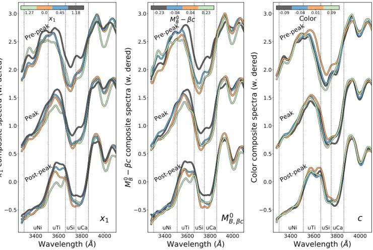
3.2. Spectroscopic variations with common SN Ia properties Here we examine how the U-band varies with commonly used SN Ia properties by comparing composite spectra generated

from subsets of the data. These are shown in Figs. 4 and 5. Subsets are constructed as follows: We retrieve all (restframe) spectra within a phase bin and normalize using the median flux of the BSNf band. If a SN has two spectra from different nights

within this range, the closest to the center of the bin is used. If the mean phase of two (sequential) spectra is closer to the cen-ter phase, their mean spectrum is used instead. At each phase we show four composite spectra constructed by dividing the full sample according to quartiles made from a secondary property, i.e. the 25% SNe with lowest value form one subset, the next 25% another and so forth. Quartile mean composites are shown, from low to high, with increasingly lighter colors (inverted for x1). A spectral feature correlation with the secondary property,

spanning the full sample and not driven by outliers, will lead to all subset composites being arranged in "color" order. Through examination of these panels we observe the following:

– x1 and M0_B,βc (lighcurve width/luminosity): The shallow

In-termediate Mass Element (IME) features of slow-declining supernovae are seen in the Ca h&k λ 3945 feature at all times (lightly shaded line). Besides this, the dominant feature is the strong correlation of the uTi-feature flux level with luminos-ity/lightcurve width. This dependence grows stronger after peak.

– Color: We find no signs of persistent feature variations with SALT2.4 color after dereddening, thus visually confirming that our dereddening procedure worked as intended. – SALT2.4 standardization residuals: We identify the pre-peak

uCa and uTi indices as potentially interesting for use in stan-dardization.

– EW(Si ii λ6355): The width of several features vary with EW(Si ii λ6355), including Ca h&k+Si ii, EW(Si ii λ4138), and uTi at late phases. This suggests that the Branch et al. (2006) subdivision into SNe Ia with broader/narrower spec-tral features is present, to some extent, in the U-band. – v(Si ii λ6355): As expected, SNe Ia with large Si velocities

at peak also demonstrate blueshifting in the Si ii λ3858 and Si ii λ4138 features.

4. Results: Understanding the explosion

4.1. Origin of U-band index variations

We use synthetic SYNAPPS fits to determine which element changes are needed to remove the dissimilarities between the SN2011fe and SN20080514-002 spectra. SYNAPPS is a C im-plementation of the original Synow code (syn++) with an added optimizer, to find the best ion temperature, velocity and opti-cal depth combinations to fit input spectra under the Sobolev approximation for e−scattering (Thomas et al. 2011). Fits pre-sented here include Mg ii, Si ii, Si iii, S ii, Ca ii, Ti ii, Fe ii, Fe iii, Cr ii, Co ii, Co iii , Ni ii. We focus on the region bluewards of the Ca h&k+Si ii region and thus do not attempt to reconstruct Ca h&k+Si ii HVFs. No detached ions were included. The full fits including these ions capture the observed spectra well. Fits were also remade while iteratively deactivating one (or a combi-nation) of the ions.

4.1.1.λ(uNi): 3300 – 3510 Å

SYNAPPS fits and their implication for the λ(uNi) spectroscopic region are shown in Fig. 6. We find that the λ(uNi) window can be tied to the presence of Ni and Co , the decay product of56Ni at these phases. Other elements, investigated using SYNAPPS runs

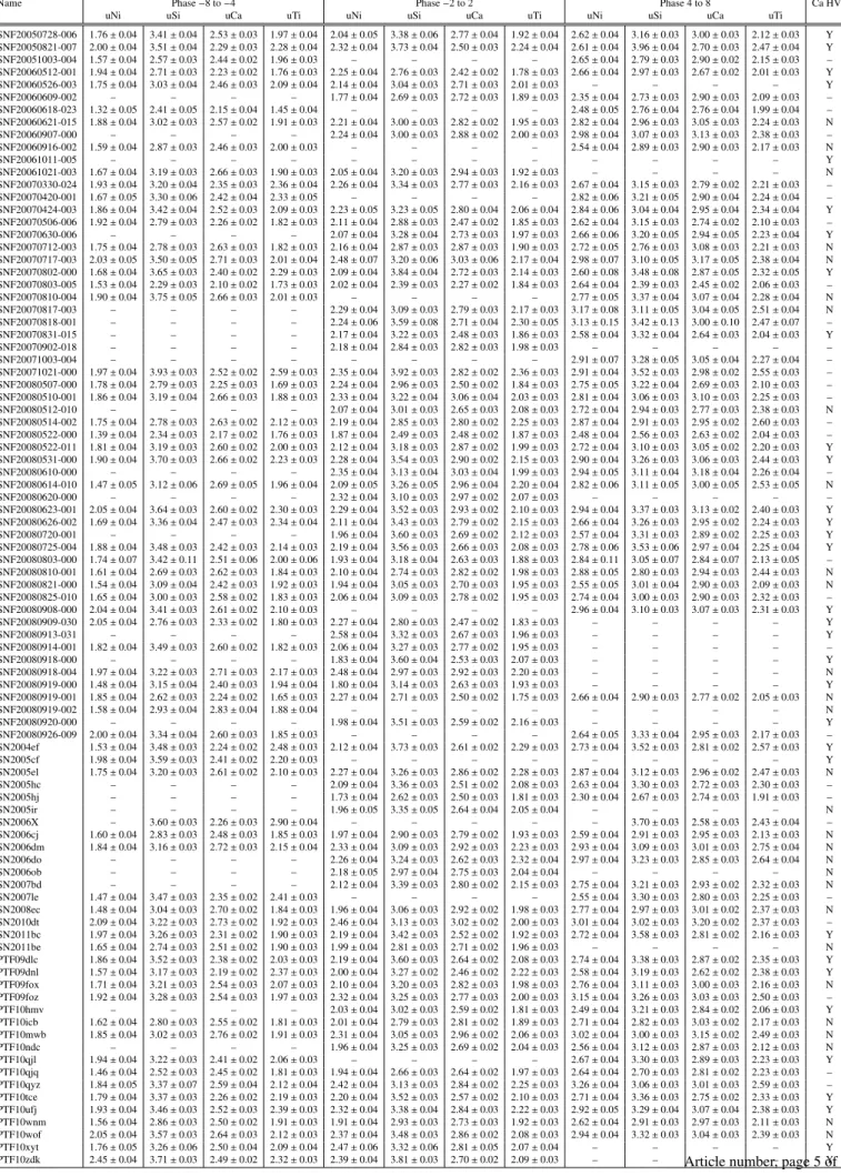
Table 1. SN U-band properties and Ca High Velocity Feature classification.

Name Phase −8 to −4 Phase −2 to 2 Phase 4 to 8 Ca HVF

uNi uSi uCa uTi uNi uSi uCa uTi uNi uSi uCa uTi

SNF20050728-006 1.76 ± 0.04 3.41 ± 0.04 2.53 ± 0.03 1.97 ± 0.04 2.04 ± 0.05 3.38 ± 0.06 2.77 ± 0.04 1.92 ± 0.04 2.62 ± 0.04 3.16 ± 0.03 3.00 ± 0.03 2.12 ± 0.03 Y SNF20050821-007 2.00 ± 0.04 3.51 ± 0.04 2.29 ± 0.03 2.28 ± 0.04 2.32 ± 0.04 3.73 ± 0.04 2.50 ± 0.03 2.24 ± 0.04 2.61 ± 0.04 3.96 ± 0.04 2.70 ± 0.03 2.47 ± 0.04 Y SNF20051003-004 1.57 ± 0.04 2.57 ± 0.03 2.44 ± 0.02 1.96 ± 0.03 – – – – 2.65 ± 0.04 2.79 ± 0.03 2.90 ± 0.02 2.15 ± 0.03 – SNF20060512-001 1.94 ± 0.04 2.71 ± 0.03 2.23 ± 0.02 1.76 ± 0.03 2.25 ± 0.04 2.76 ± 0.03 2.42 ± 0.02 1.78 ± 0.03 2.66 ± 0.04 2.97 ± 0.03 2.67 ± 0.02 2.01 ± 0.03 Y SNF20060526-003 1.75 ± 0.04 3.03 ± 0.04 2.46 ± 0.03 2.09 ± 0.04 2.14 ± 0.04 3.04 ± 0.03 2.71 ± 0.03 2.01 ± 0.03 – – – – Y SNF20060609-002 – – – – 1.77 ± 0.04 2.69 ± 0.03 2.72 ± 0.03 1.89 ± 0.03 2.35 ± 0.04 2.73 ± 0.03 2.90 ± 0.03 2.09 ± 0.03 – SNF20060618-023 1.32 ± 0.05 2.41 ± 0.05 2.15 ± 0.04 1.45 ± 0.04 – – – – 2.48 ± 0.05 2.76 ± 0.04 2.76 ± 0.04 1.99 ± 0.04 – SNF20060621-015 1.88 ± 0.04 3.02 ± 0.03 2.57 ± 0.02 1.91 ± 0.03 2.21 ± 0.04 3.00 ± 0.03 2.82 ± 0.02 1.95 ± 0.03 2.82 ± 0.04 2.96 ± 0.03 3.05 ± 0.03 2.24 ± 0.03 N SNF20060907-000 – – – – 2.24 ± 0.04 3.00 ± 0.03 2.88 ± 0.02 2.00 ± 0.03 2.98 ± 0.04 3.07 ± 0.03 3.13 ± 0.03 2.38 ± 0.03 – SNF20060916-002 1.59 ± 0.04 2.87 ± 0.03 2.46 ± 0.03 2.00 ± 0.03 – – – – 2.54 ± 0.04 2.89 ± 0.03 2.90 ± 0.03 2.17 ± 0.03 N SNF20061011-005 – – – – – – – – – – – – Y SNF20061021-003 1.67 ± 0.04 3.19 ± 0.03 2.66 ± 0.03 1.90 ± 0.03 2.05 ± 0.04 3.20 ± 0.03 2.94 ± 0.03 1.92 ± 0.03 – – – – N SNF20070330-024 1.93 ± 0.04 3.20 ± 0.04 2.35 ± 0.03 2.36 ± 0.04 2.26 ± 0.04 3.34 ± 0.03 2.77 ± 0.03 2.16 ± 0.03 2.67 ± 0.04 3.15 ± 0.03 2.79 ± 0.02 2.21 ± 0.03 – SNF20070420-001 1.67 ± 0.05 3.30 ± 0.06 2.42 ± 0.04 2.33 ± 0.05 – – – – 2.82 ± 0.06 3.21 ± 0.05 2.90 ± 0.04 2.24 ± 0.04 – SNF20070424-003 1.86 ± 0.04 3.42 ± 0.04 2.52 ± 0.03 2.09 ± 0.03 2.23 ± 0.05 3.23 ± 0.05 2.80 ± 0.04 2.06 ± 0.04 2.84 ± 0.06 3.04 ± 0.04 2.95 ± 0.04 2.34 ± 0.04 Y SNF20070506-006 1.92 ± 0.04 2.79 ± 0.03 2.26 ± 0.02 1.82 ± 0.03 2.11 ± 0.04 2.88 ± 0.03 2.47 ± 0.02 1.85 ± 0.03 2.62 ± 0.04 3.15 ± 0.03 2.74 ± 0.02 2.10 ± 0.03 – SNF20070630-006 – – – – 2.07 ± 0.04 3.28 ± 0.04 2.73 ± 0.03 1.97 ± 0.03 2.66 ± 0.06 3.20 ± 0.05 2.94 ± 0.05 2.23 ± 0.04 Y SNF20070712-003 1.75 ± 0.04 2.78 ± 0.03 2.63 ± 0.03 1.82 ± 0.03 2.16 ± 0.04 2.87 ± 0.03 2.87 ± 0.03 1.90 ± 0.03 2.72 ± 0.05 2.76 ± 0.03 3.08 ± 0.03 2.21 ± 0.03 N SNF20070717-003 2.03 ± 0.05 3.50 ± 0.05 2.71 ± 0.03 2.01 ± 0.04 2.48 ± 0.07 3.20 ± 0.06 3.03 ± 0.06 2.17 ± 0.04 2.98 ± 0.07 3.10 ± 0.05 3.17 ± 0.05 2.38 ± 0.04 N SNF20070802-000 1.68 ± 0.04 3.65 ± 0.03 2.40 ± 0.02 2.29 ± 0.03 2.09 ± 0.04 3.84 ± 0.04 2.72 ± 0.03 2.14 ± 0.03 2.60 ± 0.08 3.48 ± 0.08 2.87 ± 0.05 2.32 ± 0.05 Y SNF20070803-005 1.53 ± 0.04 2.29 ± 0.03 2.10 ± 0.02 1.73 ± 0.03 2.02 ± 0.04 2.39 ± 0.03 2.27 ± 0.02 1.84 ± 0.03 2.64 ± 0.04 2.39 ± 0.03 2.45 ± 0.02 2.06 ± 0.03 – SNF20070810-004 1.90 ± 0.04 3.75 ± 0.05 2.66 ± 0.03 2.01 ± 0.03 – – – – 2.77 ± 0.05 3.37 ± 0.04 3.07 ± 0.04 2.28 ± 0.04 N SNF20070817-003 – – – – 2.29 ± 0.04 3.09 ± 0.03 2.79 ± 0.03 2.17 ± 0.03 3.17 ± 0.08 3.11 ± 0.05 3.04 ± 0.05 2.51 ± 0.04 N SNF20070818-001 – – – – 2.24 ± 0.06 3.59 ± 0.08 2.71 ± 0.04 2.30 ± 0.05 3.13 ± 0.15 3.42 ± 0.13 3.00 ± 0.10 2.47 ± 0.07 – SNF20070831-015 – – – – 2.17 ± 0.04 3.22 ± 0.03 2.48 ± 0.03 1.86 ± 0.03 2.58 ± 0.04 3.32 ± 0.04 2.64 ± 0.03 2.04 ± 0.03 Y SNF20070902-018 – – – – 2.18 ± 0.04 2.84 ± 0.03 2.82 ± 0.03 1.98 ± 0.03 – – – – – SNF20071003-004 – – – – – – – – 2.91 ± 0.07 3.28 ± 0.05 3.05 ± 0.04 2.27 ± 0.04 – SNF20071021-000 1.97 ± 0.04 3.93 ± 0.03 2.52 ± 0.02 2.59 ± 0.03 2.35 ± 0.04 3.92 ± 0.03 2.82 ± 0.02 2.36 ± 0.03 2.91 ± 0.04 3.52 ± 0.03 2.98 ± 0.02 2.55 ± 0.03 – SNF20080507-000 1.78 ± 0.04 2.79 ± 0.03 2.25 ± 0.03 1.69 ± 0.03 2.24 ± 0.04 2.96 ± 0.03 2.50 ± 0.02 1.84 ± 0.03 2.75 ± 0.05 3.22 ± 0.04 2.69 ± 0.03 2.10 ± 0.03 – SNF20080510-001 1.86 ± 0.04 3.19 ± 0.04 2.66 ± 0.03 1.88 ± 0.03 2.33 ± 0.04 3.22 ± 0.04 3.06 ± 0.04 2.03 ± 0.03 2.81 ± 0.04 3.06 ± 0.03 3.10 ± 0.03 2.25 ± 0.03 – SNF20080512-010 – – – – 2.07 ± 0.04 3.01 ± 0.03 2.65 ± 0.03 2.08 ± 0.03 2.72 ± 0.04 2.94 ± 0.03 2.77 ± 0.03 2.38 ± 0.03 N SNF20080514-002 1.75 ± 0.04 2.78 ± 0.03 2.63 ± 0.02 2.12 ± 0.03 2.19 ± 0.04 2.85 ± 0.03 2.80 ± 0.02 2.25 ± 0.03 2.87 ± 0.04 2.91 ± 0.03 2.95 ± 0.02 2.60 ± 0.03 – SNF20080522-000 1.39 ± 0.04 2.34 ± 0.03 2.17 ± 0.02 1.76 ± 0.03 1.87 ± 0.04 2.49 ± 0.03 2.48 ± 0.02 1.87 ± 0.03 2.48 ± 0.04 2.56 ± 0.03 2.63 ± 0.02 2.04 ± 0.03 – SNF20080522-011 1.81 ± 0.04 3.19 ± 0.03 2.60 ± 0.02 2.00 ± 0.03 2.12 ± 0.04 3.18 ± 0.03 2.87 ± 0.02 1.99 ± 0.03 2.72 ± 0.04 3.10 ± 0.03 3.05 ± 0.02 2.20 ± 0.03 Y SNF20080531-000 1.90 ± 0.04 3.70 ± 0.03 2.66 ± 0.02 2.23 ± 0.03 2.28 ± 0.04 3.54 ± 0.03 2.90 ± 0.02 2.15 ± 0.03 2.90 ± 0.04 3.26 ± 0.03 3.06 ± 0.03 2.44 ± 0.03 Y SNF20080610-000 – – – – 2.35 ± 0.04 3.13 ± 0.04 3.03 ± 0.04 1.99 ± 0.03 2.94 ± 0.05 3.11 ± 0.04 3.18 ± 0.04 2.26 ± 0.04 – SNF20080614-010 1.47 ± 0.05 3.12 ± 0.06 2.69 ± 0.05 1.96 ± 0.04 2.09 ± 0.05 3.26 ± 0.05 2.96 ± 0.04 2.20 ± 0.04 2.82 ± 0.06 3.11 ± 0.05 3.00 ± 0.05 2.53 ± 0.05 N SNF20080620-000 – – – – 2.32 ± 0.04 3.10 ± 0.03 2.97 ± 0.02 2.07 ± 0.03 – – – – – SNF20080623-001 2.05 ± 0.04 3.64 ± 0.03 2.60 ± 0.02 2.30 ± 0.03 2.29 ± 0.04 3.52 ± 0.03 2.93 ± 0.02 2.10 ± 0.03 2.94 ± 0.04 3.37 ± 0.03 3.13 ± 0.02 2.40 ± 0.03 Y SNF20080626-002 1.69 ± 0.04 3.36 ± 0.04 2.47 ± 0.03 2.34 ± 0.04 2.11 ± 0.04 3.43 ± 0.03 2.79 ± 0.02 2.15 ± 0.03 2.66 ± 0.04 3.26 ± 0.03 2.95 ± 0.02 2.24 ± 0.03 Y SNF20080720-001 – – – – 1.96 ± 0.04 3.60 ± 0.03 2.69 ± 0.02 2.12 ± 0.03 2.57 ± 0.04 3.31 ± 0.03 2.89 ± 0.02 2.25 ± 0.03 Y SNF20080725-004 1.88 ± 0.04 3.48 ± 0.03 2.42 ± 0.03 2.14 ± 0.03 2.19 ± 0.04 3.56 ± 0.03 2.66 ± 0.03 2.08 ± 0.03 2.78 ± 0.06 3.53 ± 0.06 2.97 ± 0.04 2.25 ± 0.04 Y SNF20080803-000 1.74 ± 0.07 3.42 ± 0.11 2.51 ± 0.06 2.00 ± 0.06 1.93 ± 0.04 3.18 ± 0.04 2.63 ± 0.03 1.88 ± 0.03 2.84 ± 0.11 3.05 ± 0.07 2.84 ± 0.07 2.13 ± 0.05 – SNF20080810-001 1.61 ± 0.04 2.69 ± 0.03 2.62 ± 0.03 1.84 ± 0.03 2.10 ± 0.04 2.74 ± 0.03 2.82 ± 0.02 1.98 ± 0.03 2.88 ± 0.05 2.80 ± 0.03 2.94 ± 0.03 2.44 ± 0.03 N SNF20080821-000 1.54 ± 0.04 3.09 ± 0.04 2.42 ± 0.03 1.92 ± 0.03 1.94 ± 0.04 3.05 ± 0.03 2.70 ± 0.03 1.95 ± 0.03 2.55 ± 0.05 3.01 ± 0.04 2.90 ± 0.03 2.09 ± 0.03 N SNF20080825-010 1.65 ± 0.04 3.00 ± 0.03 2.58 ± 0.02 1.83 ± 0.03 2.06 ± 0.04 3.09 ± 0.03 2.78 ± 0.02 1.95 ± 0.03 2.74 ± 0.04 3.00 ± 0.03 2.90 ± 0.03 2.32 ± 0.03 – SNF20080908-000 2.04 ± 0.04 3.41 ± 0.03 2.61 ± 0.02 2.10 ± 0.03 – – – – 2.96 ± 0.04 3.10 ± 0.03 3.07 ± 0.03 2.31 ± 0.03 Y SNF20080909-030 2.05 ± 0.04 2.76 ± 0.03 2.33 ± 0.02 1.80 ± 0.03 2.27 ± 0.04 2.80 ± 0.03 2.47 ± 0.02 1.83 ± 0.03 – – – – Y SNF20080913-031 – – – – 2.58 ± 0.04 3.32 ± 0.03 2.67 ± 0.03 1.96 ± 0.03 – – – – Y SNF20080914-001 1.82 ± 0.04 3.49 ± 0.03 2.60 ± 0.02 1.82 ± 0.03 2.06 ± 0.04 3.27 ± 0.03 2.77 ± 0.02 1.95 ± 0.03 – – – – – SNF20080918-000 – – – – 1.83 ± 0.04 3.60 ± 0.04 2.53 ± 0.03 2.07 ± 0.03 – – – – Y SNF20080918-004 1.97 ± 0.04 3.22 ± 0.03 2.71 ± 0.03 2.17 ± 0.03 2.48 ± 0.04 2.97 ± 0.03 2.92 ± 0.03 2.20 ± 0.03 – – – – N SNF20080919-000 1.48 ± 0.04 3.15 ± 0.04 2.40 ± 0.03 1.94 ± 0.04 1.80 ± 0.04 3.14 ± 0.03 2.63 ± 0.03 1.93 ± 0.03 – – – – Y SNF20080919-001 1.85 ± 0.04 2.62 ± 0.03 2.24 ± 0.02 1.65 ± 0.03 2.27 ± 0.04 2.71 ± 0.03 2.50 ± 0.02 1.75 ± 0.03 2.66 ± 0.04 2.90 ± 0.03 2.77 ± 0.02 2.05 ± 0.03 N SNF20080919-002 1.58 ± 0.04 2.93 ± 0.04 2.83 ± 0.04 1.88 ± 0.04 – – – – – – – – N SNF20080920-000 – – – – 1.98 ± 0.04 3.51 ± 0.03 2.59 ± 0.02 2.16 ± 0.03 – – – – Y SNF20080926-009 2.00 ± 0.04 3.34 ± 0.04 2.60 ± 0.03 1.85 ± 0.03 – – – – 2.64 ± 0.05 3.33 ± 0.04 2.95 ± 0.03 2.17 ± 0.03 – SN2004ef 1.53 ± 0.04 3.48 ± 0.03 2.24 ± 0.02 2.48 ± 0.03 2.12 ± 0.04 3.73 ± 0.03 2.61 ± 0.02 2.29 ± 0.03 2.73 ± 0.04 3.52 ± 0.03 2.81 ± 0.02 2.57 ± 0.03 Y SN2005cf 1.98 ± 0.04 3.59 ± 0.03 2.41 ± 0.02 2.20 ± 0.03 – – – – – – – – Y SN2005el 1.75 ± 0.04 3.20 ± 0.03 2.61 ± 0.02 2.10 ± 0.03 2.27 ± 0.04 3.26 ± 0.03 2.86 ± 0.02 2.28 ± 0.03 2.87 ± 0.04 3.12 ± 0.03 2.96 ± 0.02 2.47 ± 0.03 N SN2005hc – – – – 2.09 ± 0.04 3.36 ± 0.03 2.51 ± 0.02 2.08 ± 0.03 2.63 ± 0.04 3.30 ± 0.03 2.72 ± 0.03 2.30 ± 0.03 – SN2005hj – – – – 1.73 ± 0.04 2.62 ± 0.03 2.50 ± 0.03 1.81 ± 0.03 2.30 ± 0.04 2.67 ± 0.03 2.74 ± 0.03 1.91 ± 0.03 – SN2005ir – – – – 1.96 ± 0.05 3.35 ± 0.05 2.64 ± 0.04 2.05 ± 0.04 – – – – N SN2006X – 3.60 ± 0.03 2.26 ± 0.03 2.90 ± 0.04 – – – – – 3.70 ± 0.03 2.58 ± 0.03 2.43 ± 0.04 – SN2006cj 1.60 ± 0.04 2.83 ± 0.03 2.48 ± 0.03 1.85 ± 0.03 1.97 ± 0.04 2.90 ± 0.03 2.79 ± 0.02 1.93 ± 0.03 2.59 ± 0.04 2.91 ± 0.03 2.95 ± 0.03 2.13 ± 0.03 N SN2006dm 1.84 ± 0.04 3.16 ± 0.03 2.72 ± 0.03 2.15 ± 0.04 2.33 ± 0.04 3.09 ± 0.03 2.92 ± 0.03 2.23 ± 0.03 2.93 ± 0.04 3.09 ± 0.03 3.01 ± 0.03 2.75 ± 0.04 N SN2006do – – – – 2.26 ± 0.04 3.24 ± 0.03 2.62 ± 0.03 2.32 ± 0.04 2.97 ± 0.04 3.23 ± 0.03 2.85 ± 0.03 2.64 ± 0.04 N SN2006ob – – – – 2.18 ± 0.05 2.97 ± 0.04 2.75 ± 0.03 2.04 ± 0.04 – – – – N SN2007bd – – – – 2.12 ± 0.04 3.39 ± 0.03 2.80 ± 0.02 2.15 ± 0.03 2.75 ± 0.04 3.21 ± 0.03 2.93 ± 0.02 2.32 ± 0.03 N SN2007le 1.47 ± 0.04 3.47 ± 0.03 2.35 ± 0.02 2.41 ± 0.03 – – – – 2.55 ± 0.04 3.30 ± 0.03 2.80 ± 0.03 2.25 ± 0.03 – SN2008ec 1.48 ± 0.04 3.04 ± 0.03 2.70 ± 0.02 1.84 ± 0.03 1.96 ± 0.04 3.06 ± 0.03 2.92 ± 0.02 1.98 ± 0.03 2.77 ± 0.04 2.97 ± 0.03 3.01 ± 0.02 2.37 ± 0.03 N SN2010dt 2.09 ± 0.04 3.22 ± 0.03 2.73 ± 0.02 1.92 ± 0.03 2.46 ± 0.04 3.13 ± 0.03 3.02 ± 0.02 2.00 ± 0.03 3.01 ± 0.04 3.02 ± 0.03 3.20 ± 0.02 2.37 ± 0.03 – SN2011bc 1.97 ± 0.04 3.26 ± 0.03 2.31 ± 0.02 1.90 ± 0.03 2.19 ± 0.04 3.42 ± 0.03 2.52 ± 0.02 1.92 ± 0.03 2.72 ± 0.04 3.58 ± 0.03 2.81 ± 0.02 2.16 ± 0.03 Y SN2011be 1.65 ± 0.04 2.74 ± 0.03 2.51 ± 0.02 1.90 ± 0.03 1.99 ± 0.04 2.81 ± 0.03 2.71 ± 0.02 1.96 ± 0.03 – – – – N PTF09dlc 1.86 ± 0.04 3.52 ± 0.03 2.38 ± 0.02 2.03 ± 0.03 2.19 ± 0.04 3.60 ± 0.03 2.64 ± 0.02 2.08 ± 0.03 2.74 ± 0.04 3.38 ± 0.03 2.87 ± 0.02 2.35 ± 0.03 Y PTF09dnl 1.57 ± 0.04 3.17 ± 0.03 2.19 ± 0.02 2.37 ± 0.03 2.00 ± 0.04 3.27 ± 0.02 2.46 ± 0.02 2.22 ± 0.03 2.58 ± 0.04 3.19 ± 0.03 2.62 ± 0.02 2.38 ± 0.03 Y PTF09fox 1.71 ± 0.04 3.21 ± 0.03 2.54 ± 0.03 2.07 ± 0.03 2.10 ± 0.04 3.20 ± 0.03 2.82 ± 0.03 1.98 ± 0.03 2.76 ± 0.04 3.11 ± 0.03 3.00 ± 0.03 2.16 ± 0.03 N PTF09foz 1.92 ± 0.04 3.28 ± 0.03 2.54 ± 0.03 1.97 ± 0.03 2.32 ± 0.04 3.25 ± 0.03 2.77 ± 0.03 2.00 ± 0.03 3.15 ± 0.04 3.26 ± 0.03 3.03 ± 0.03 2.50 ± 0.03 – PTF10hmv – – – – 2.03 ± 0.04 3.02 ± 0.03 2.59 ± 0.02 1.81 ± 0.03 2.49 ± 0.04 3.21 ± 0.03 2.84 ± 0.02 2.06 ± 0.03 Y PTF10icb 1.62 ± 0.04 2.80 ± 0.03 2.55 ± 0.02 1.81 ± 0.03 2.01 ± 0.04 2.79 ± 0.03 2.81 ± 0.02 1.89 ± 0.03 2.71 ± 0.04 2.82 ± 0.03 3.03 ± 0.02 2.17 ± 0.03 N PTF10mwb 1.85 ± 0.04 3.02 ± 0.03 2.76 ± 0.02 1.91 ± 0.03 2.31 ± 0.04 3.05 ± 0.03 2.96 ± 0.02 2.06 ± 0.03 3.02 ± 0.04 3.00 ± 0.03 3.15 ± 0.02 2.49 ± 0.03 N PTF10ndc – – – – 1.96 ± 0.04 3.25 ± 0.03 2.69 ± 0.02 2.04 ± 0.03 2.56 ± 0.04 3.12 ± 0.03 2.87 ± 0.03 2.12 ± 0.03 N PTF10qjl 1.94 ± 0.04 3.22 ± 0.03 2.41 ± 0.02 2.06 ± 0.03 – – – – 2.67 ± 0.04 3.30 ± 0.03 2.89 ± 0.03 2.23 ± 0.03 Y PTF10qjq 1.46 ± 0.04 2.52 ± 0.03 2.45 ± 0.02 1.81 ± 0.03 1.94 ± 0.04 2.66 ± 0.03 2.64 ± 0.02 1.97 ± 0.03 2.64 ± 0.04 2.70 ± 0.03 2.81 ± 0.02 2.23 ± 0.03 – PTF10qyz 1.84 ± 0.05 3.37 ± 0.07 2.59 ± 0.04 2.12 ± 0.04 2.42 ± 0.04 3.13 ± 0.03 2.84 ± 0.02 2.25 ± 0.03 3.26 ± 0.04 3.06 ± 0.03 3.01 ± 0.03 2.59 ± 0.03 – PTF10tce 1.79 ± 0.04 3.37 ± 0.03 2.26 ± 0.02 2.19 ± 0.03 2.20 ± 0.04 3.52 ± 0.03 2.57 ± 0.02 2.10 ± 0.03 2.71 ± 0.04 3.36 ± 0.03 2.75 ± 0.02 2.33 ± 0.03 Y PTF10ufj 1.93 ± 0.04 3.46 ± 0.03 2.52 ± 0.03 2.39 ± 0.03 2.32 ± 0.04 3.38 ± 0.04 2.84 ± 0.03 2.22 ± 0.03 2.92 ± 0.05 3.29 ± 0.04 3.07 ± 0.04 2.38 ± 0.03 Y PTF10wnm 1.56 ± 0.04 2.86 ± 0.03 2.50 ± 0.02 1.91 ± 0.03 1.91 ± 0.04 2.93 ± 0.03 2.73 ± 0.03 1.92 ± 0.03 2.62 ± 0.04 2.91 ± 0.03 2.97 ± 0.03 2.11 ± 0.03 N PTF10wof 2.05 ± 0.04 3.57 ± 0.03 2.64 ± 0.03 2.12 ± 0.03 2.37 ± 0.04 3.48 ± 0.03 2.86 ± 0.02 2.08 ± 0.03 2.94 ± 0.04 3.32 ± 0.03 3.04 ± 0.03 2.39 ± 0.03 N PTF10xyt 1.76 ± 0.05 3.26 ± 0.06 2.50 ± 0.04 2.09 ± 0.04 2.47 ± 0.06 3.32 ± 0.06 2.81 ± 0.05 2.07 ± 0.04 – – – – Y PTF10zdk 2.45 ± 0.04 3.71 ± 0.03 2.49 ± 0.02 2.32 ± 0.03 2.39 ± 0.04 3.81 ± 0.03 2.70 ± 0.02 2.09 ± 0.03 – – – – Y

Notes. See 2.3 for parameter definitions and 6.1 for HVF classification.

3300 3500

4000

5000

6000

Wavelength (Å, restframe)

0.2

0.4

0.6

0.8

1.0

1.2

1.4

1.6

1.8

Flux density (normalized)

Fe

Fe

3300 3500

4000

5000

6000

Wavelength (Å, restframe)

0.2

0.4

0.6

0.8

1.0

1.2

1.4

1.6

1.8

Flux density (normalized)

SN2011fe @ peak light SNF200805014-002 @ peak light

Fig. 1. Comparison of the spectra of SN2011fe (SALT2.4 x1= −0.4 and c = −0.06) and SNF200805014-002 (SALT2.4 x1= −1.5 and c = −0.12)

at early (left) and peak (right) phases. Small spectroscopic differences are found redwards of 4000 Å (stable Fe marked in left panel). Much larger deviation is found bluewards of this limit. The comparison at early phases differs most strongly around 3400 Å and the high velocity edge of the Ca h&k λ 3945 feature, the comparison at later phases mainly around 3550 Å. These differences led to the subdivision of the U-band into four indices, as described in the text. Vertical lines show the feature limits thus defined.

3300

3400

3500

3600

3700

3800

3900

Wavelength (Å, restframe)

0.0

0.5

1.0

1.5

2.0

2.5

Normalized flux density

uNi

uTi

uSi

uCa

Pre-peak (-8 to -4 days)

Peak (-2 to 2 days)

Post-peak (4 to 8 days)

Fig. 2. Mean spectra and ±1 standard deviation in sample at three representative phases. The four wavelength regions considered are separated by dashed lines. The interpretation of these indices will be phase dependent, as e.g. the Ti region at early phases is clearly a part of the Ca h&k λ 3945 + Si ii λ3858 feature complex and Cr/Fe dominates uNi at late phases.

without Ni/Co, cannot replicate the observed spectra without dis-torting other parts of the spectrum. The effects of Ni and Co can be directly seen by manually decreasing the optical depths of these ions relative to the SN2011fe fit: a change of order 1 dex creates a syn++ spectrum that matches SNF20080514-002 well in the λ(uNi) region (lower panels of Fig. 6). We show con-tributions of all included ions to the full fit in the Appendix (Figure A.1). Tanaka et al. (2008), using abundance modifica-tions to the W7 density profile to fit SN2002bo, also found this wavelength region to be sensitive to the amount of outer Ni (see their Fig. 2). Similar results can be seen in a number of studies using different techniques: Blondin et al. (2013) presented one-dimensional delayed-detonation models that show Co ii to dom-inate here; Hachinger et al. (2013) performed a spectral tomog-raphy analysis of SN2010jn where an early spectrum was

domi-nated by Fe absorption at 3000 Å and the Ni/Co around 3200 Å, and a SYNAPPS study by Smitka et al. (2015) also shows strong Ni/Co absorption at ∼ 3300 Å (although no Cr or Ti was in-cluded in these fits). Like Hachinger et al. (2013), we find that measurements of this spectral region are necessary for determin-ing the spatial distribution of IGE elements, a key characteristic distinguishing theoretical explosion models. Cartier et al. (2017) found that V ii provided improved fits to very early spectra of SN2015F, which would also impact the λ(uNi) region.

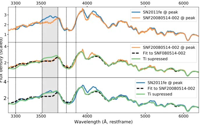
4.1.2. uTi : 3510 – 3660 Å

SYNAPPS fits and their implication for the λ(uTi) region are shown in Fig. 7. Among the SYNAPPS ions included, only Ti ii produces significant absorption in the 3510 to 3660 Å region

3300

3500

4000

5000

6000

Wavelength (Å, dereddened)

0

0.2

0.4

0.6

Pre-peak: [-8,-4]

-0.65

0.05

0.75

1.45

x

1

3300

3500

4000

5000

6000

Wavelength (Å, dereddened)

0

0.2

0.4

0.6

RM

S

of

n

or

m

ali

ze

d

flu

x d

en

sit

y f

or

x

1

su

bs

et

s

Peak: [-2,2]

3300

3500

4000

5000

6000

Wavelength (Å, restframe)

0

0.2

0.4

0.6

uNi

uTi uSi uCa

Post-peak: [4,8]

Full sample RMS

Fig. 3. Intrinsic flux RMS (vs. wavelength) for SNe after division into four bins according to increasing lightcurve width (dark to light lines). Spectra were initially normalized to have median flux of unity over the [3300, 6900] Å wavelength region. Panels from top to bottom show the three sample phase regions (pre-peak, peak and post-peak). Vertical (dotted) lines mark boundaries of the four U-band regions. The red dashed red line shows the RMS for the full sample.

without distorting other parts of the spectrum. We display this association by manually decreasing the Ti ii optical depth. We do this for SNF20080514-002 since it shows the larger absorp-tion, and again find that a change of order −1 dex produces a spectrum that matches the SN2011fe uTi region well. More com-plete radiative transfer models are needed to determine whether uTi variations are fully explained by Ti ii absorption, but we note that the Ti lines at 3685, 3759 and 3761 Å would land in the uTi wavelength region for typical SN Ia velocities. The post-peak λ(uTi) region is, as can be seen in Figs. 4 and 5, strongly corre-lated with EW(Si ii λ6355). As no strong Si lines are expected in this region this reflects a general connection between widths of

spectroscopic features in SN Ia spectra. We show contributions of all included ions to the full fit in the Appendix (Fig. AA.2).

4.2. Explosion models and progenitor scenarios

The single degenerate scenario – mass transfer from a red giant or main sequence star onto a Carbon-Oxygen White Dwarf – is no longer considered as likely to explain all (or most) SNe Ia. Challenges come from the lack of companion stars close to nearby SNe (e.g. SN2011fe Li et al. 2011; Schaefer & Pag-notta 2012; Edwards et al. 2012), the statistical absence of early lightcurve variations due to ejecta interaction with the

3400 3600 3800 4000

Wavelength (Å)

0.5

0.0

0.5

1.0

1.5

2.0

2.5

3.0

x

1

co

m

po

sit

e s

pe

ctr

a (

w.

d

er

ed

)

Pre-peak

Peak

Post-peak

x

1

uNi

uTi uSi uCa

-1.27 0.0 0.45 1.18

x

3400 3600 3800 4000

Wavelength (Å)

0.5

0.0

0.5

1.0

1.5

2.0

2.5

3.0

M

0 B

c c

om

po

sit

e s

pe

ctr

a (

w.

d

er

ed

)

Pre-peak

Peak

Post-peak

M

_{B, c}

0

uNi

uTi uSi uCa

-0.23 -0.04 0.04 0.23

M

c

3400 3600 3800 4000

Wavelength (Å)

0.5

0.0

0.5

1.0

1.5

2.0

2.5

3.0

Color composite spectra (w. dered)

Pre-peak

Peak

Post-peak

c

uNi

uTi uSi uCa

-0.09 -0.04 0.01 0.09

Color

Fig. 4. U-band spectroscopic variation spanning the range of common SN properties: x1, dereddened MB, Color (left to right). Composite spectra

were calculated after dividing the sample into four quartiles based on each property, which was repeated at three representative phase ranges (−6, 0, 6) for each subset. Subset composites were drawn such that the line color becomes darker as the parameter value decreases. Dotted lines indicate U-band spectral-index sub division boundaries.

ion (Hayden et al. 2010), an insufficient number of such systems formed (Ruiter et al. 2011), and a large range of ejecta masses (Scalzo et al. 2014). A number of scenarios, possibly existing in parallel, are currently being investigated. These predict similar spectral energy distributions in the 4000 to 7000 Å region around lightcurve peak and have thus proven hard to rule out using such data (Röpke et al. 2012). Bluer wavelengths, on the other hand, show significant differences between current theoretical mod-els. We have compared output spectra from delayed detonation (model N110, Seitenzahl et al. 2014; Sim et al. 2013), violent merger (model 11+09, Pakmor et al. 2012), sub-Chandra dou-ble detonation (model 3m, Kromer et al. 2010) and sub-Chandra WD detonation (Sim et al. 2010) models. We find that none of these describe the observed U-band variations.

Miles et al. (2016) found constant Si but varying Ca abun-dances to be a robust consequence of changing the progenitor model metallicity. However, they do not find this to cause strong changes in the observed spectra. We have nonetheless searched for uCa changes, not visible in uSi, for indications of a relation-ship to metallicity, but did not observe anything significant. The region identified by Miles et al. (2016) as strongly and consis-tently affected by metallicity was the Ti absorption at ∼ 4300 Å at ∼ 30 days after explosion. As this feature, as for the uTi in-dex, is strongly correlated with peak luminosity and lightcurve width, searching for a second order variation due to metallicity is challenging.

A more direct way to probe Ni in the outermost layer is through observation of the very early lightcurve rise-time, pa-rameterized as f ∝ tn_{. A mixed ejecta (shallow}56_{Ni) will cause}

an immediate, gradual flux increase while deeper56Ni with cool outer layers experience a few days of dark time before a sharply rising lightcurve (Piro & Nakar 2014; Piro & Morozova 2016). In these models, the effects of outer ejecta mixing has largely dis-appeared ∼ one week after explosion. Firth et al. (2015) examine a sample of SNe with very early observations, finding varying rise-time power-law indices n between 1.48 and 3.7, suggesting that either the outermost56Ni layer and/or the shock structure varies significantly between events. A sample of SNe with both early lightcurve data and U-band spectra would allow a direct comparison between pre-peak λ(uNi) absorption and the amount of shallow Ni predicted from the early lightcurve rise-time.

SN2011fe and LSQ12fxd in the Firth et al. (2015) study are included in the sample studied here and have observations at a common phase of ∼ 10 days before peak (shown in Fig. 8). Compared with SN2011fe, LSQ12fxd has both a steeper rise-time immediately after explosion (n = 3.24 vs. n = 2.15) and more Co ii absorption (less λ(uNi) flux) in the line-forming re-gion one week prior to lightcurve peak. A scenario explaining both observations would involve56_{Ni mixed into the outermost}

ejecta regions in SN2011fe while being located slightly deeper and being denser in LSQ12fxd. The comparison is non-trivial as these SNe also vary significantly in lightcurve width and line velocities, but we note that neither x1 nor v(Si ii λ6355)

corre-3400 3600 3800 4000

Wavelength (Å)

0.5

0.0

0.5

1.0

1.5

2.0

2.5

3.0

Hubble res. (mag) composite spectra (w. dered)

Pre-peak

Peak

Post-peak

HR

uNi

uTi uSi uCa

-0.15 -0.02 0.06 0.17

Hubble res. (mag)

3400 3600 3800 4000

Wavelength (Å)

0.5

0.0

0.5

1.0

1.5

2.0

2.5

3.0

EWSiII6355 composite spectra (w. dered)

Pre-peak

Peak

Post-peak

EW

Si

uNi

uTi uSi uCa

67.39 89.14 103.52 121.81

EWSiII6355

3400 3600 3800 4000

Wavelength (Å)

0.5

0.0

0.5

1.0

1.5

2.0

2.5

3.0

v(SiII6355) composite spectra (w. dered)

Pre-peak

Peak

Post-peak

v

Si

uNi

uTi uSi uCa

-9483 -10287 -10869 -12037

v(SiII6355)

Fig. 5. U-band spectroscopic variation spanning the range of common SN properties: Hubble residuals standardized by SALT2.4 lightcurve parameters, EW(Si ii λ6355) and v(Si ii λ6355) (left to right). Composite spectra were calculated after dividing the sample into four quartiles based on each property, which was repeated at three representative phase ranges (−6, 0, 6) for each subset. Subset composites were drawn such that the line color becomes darker as the parameter value decreases. Dotted lines indicate U-band spectral-index sub division boundaries.

lates strongly with early uNi and that Firth et al. (2015) find no correlation between n and lightcurve width.

5. Results: Impact on standardization

Here we discuss the strong correlation between post-peak uTi and peak luminosity, and the potential impact of uCa, for SN Ia standardization (Sec. 5.1). The residual magnitude correla-tion with host environment after standardizacorrela-tion is explored in Sec. 5.2. In Sec. 5.3 we explore whether the systematic effects from reddening corrections could significantly affect these re-sults.

5.1. SN Ia luminosity standardization with uTi and uCa Many spectroscopic features show strong correlations with SN Ia luminosity. These include R(Si) and R(Ca), introduced by Nu-gent et al. (1995), and the equivalent width (or “strength”) of the Si ii λ4138 feature (Arsenijevic et al. 2008; Chotard et al. 2011; Nordin et al. 2011). As discussed in Sec. 3.2, uTi displays a similarly strong sensitivity to peak luminosity, especially at post-peak phases where contamination by the blue edge of the Ca h&k λ 3945 feature is less likely. For some SNe a direct con-nection to R(Ca), measured as the ratio between flux at the edges of the Ca h&k λ 3945 feature, could exist. We now further ex-plore the uTi-luminosity correlation.

In Fig. 9 (mid panel) we show the uTi change with phase per SN, and with measurements color-coded by lightcurve width (SALT2.4 x1). From around lightcurve peak and later, we find a

persistent and strong relation, where SNe with wider lightcurves have bluer uTi colors. To confirm that this correlation is not driven by the dereddening correction or changes in the BSNf

band, Fig. 9 contains two modified color curves: The first (left panel) shows the observed color uTiobs,B, i.e. uTi recalculated

ac-cording to Equation 1 but without dereddening spectra, and the second (right panel) shows the BSNf− VSNfcolor evolution

(cal-culated based on restframe and dereddened spectra). We confirm that the strong x1trend is present also without dereddening but

not visible for BSNf− VSNf.

We evaluate SN Ia standardization using combinations of post-peak uTi as a replacement for x1, and pre-peak uCa as an

additional standardization parameter (see Table 2). We assume a fixedΛCDM cosmology, continue to remove red SNe (c > 0.2) and use SNe in the 0.03 < z < 0.1 range to reduce scatter from peculiar velocities. We further fix the SALT2.4 β param-eter (the magnitude dependence of c) to the (blinded) value de-termined from the full SNfactory sample (derived without cuts based on color or first phase). The two base fits include either the magnitude dependence of x1(“α”) or the magnitude

depen-dence of post-peak uTi. Two permutations of these are made: one (“cut”) where the sample is limited to SNe with observa-tions at all phases (early and late), and another where pre-peak uCa is added as a second standardization parameter. To allow

3300

3500

4000

5000

6000

Wavelength (A)

1

2

3

SN2011fe @ -10 days

_{SNF20080514-002 @ -10 days}

Wavelength (A)

2

4

Flux density (scaled)

SN2011fe @ -10 days

Fit to SN2011fe

Ni/Co supressed

3300

3500

4000

5000

6000

Wavelength (Å, restframe)

2

4

SNF20080514-002 @ -10 days

Fit to SN2011fe

Ni/Co supressed

Fig. 6. Probing the origin of variation in the λ(uNi) region through SYNAPPS model comparisons. The top panel compares SN2011fe and SNF20080514-002 at an early phase (−10 days). The second panel repeats the early SN2011fe spectrum (blue line) together with the best SYNAPPS fit (black dashed line). The green line shows the same fit, but with the optical depth (τ) of all Ni and Co ii decreased by one dex, effectively suppressing these ions. The third panel compares the early SNF20080514-002 spectrum with the same SN2011fe SYNAPPS fits. The SN2011fe fit with suppressed Ni , Co ii optical depth matches the SNF20080514-002 λ(uNi) region well. Vertical dotted lines indicate the U-band spectral index boundaries, with λ(uNi) lightly shaded grey.

comparisons of χ2 _{between runs we add a fixed dispersion of}

0.090 mag, the value required to produce χ2/dof = 1 for the ini-tial x1 run (first row in table). The uncertainty of each U-band

index is composed of the sum of variance due to statistical un-certainties of the spectra and the propagated reddening variance, and is generally at the ∼ 0.03 mag level (see Table 1). The mea-surement correlations between U-band indices and SALT2.4 fit parameters are negligible.

Our primary conclusion is that post-peak uTi standardizes SNe Ia very effectively, with an RMS of 0.116 ± 0.011 mag. A traditional x1 standardization yields a higher RMS of 0.135 ±

0.011 mag for these SNe. This is remarkable in many aspects: it is a single color measurement made in a fairly wide phase range and using a fixed wavelength range that produces a lower χ2fit. For the reduced sample of 57 SNe with both measurements this is an improvement over x1with∆χ2= 20.5, which is significant

at greater than 3 σ (see also Table 3). We further investigate the potential effects of sample selection by redoing the fits based on a “cut” sample, where only SNe with both pre-peak (−8 to −4 days) and post-peak (4 to 8) data are included. We see no signif-icant differences between the full and cut samples. The reduced dispersion for uTi fits is thus not due to sample selection.

The Spearman rank correlation coefficient between SALT2.4 Hubble residuals and pre-peak uCa is rs= 0.43, and the

hypoth-esis of no correlation can be rejected at greater than 99% con-fidence (Fig. 10, left panel). We therefore test adding pre-peak uCa measurements as a further standardization parameter. Com-bining post-peak uTi and pre-peak uCa produces a Hubble dia-gram RMS of 0.086 ± 0.010 mag, while using only uCa and x1

reduced the RMS to 0.122 ± 0.012 mag. The driving trend of this improvement can also be seen in Fig. 10: SNe Ia with large uCa index are too bright after SALT2.4 standardization. Half of these are classified as Branch Shallow Silicon objects – this connec-tion is further explored in Sec. 6.1.

We also note that the combined uTi + uCa fit produces a much reduced χ2 value, beyond what can be expected just through adding another fit parameter. When rerunning the stan-dardization without a fixed intrinsic dispersion we obtain χ2 = 38.6 for 40 degrees of freedom, thus there is no need to add any additional dispersion to reach χ2_{/dof = 1. As the internal}

SALT2.4 model error propagates an effective intrinsic disper-sion of 0.055 mag, other fit methods are required to investigate whether a fit without any added dispersion can be attained. For comparison, the uTi fit requires an intrinsic dispersion of σint =

0.070 ± 0.009 mag and the x1fit requires σint = 0.090 ± 0.008

mag.

As a further test we evaluate the fit quality using the sample-size corrected Akaike Information Criteria (AICc), which penal-izes models with additional fit parameters. In Table 3 each line compares uTi standardization (without any host galaxy property correction) with one other combination of standardization prop-erty and host parameter. Each comparison includes all SNe avail-able for that combination of data, and shows both the difference in χ2_{and the AICc probability ratio. Models including both uTi}

and uCa are strongly preferred over only using uTi, with a P-value of < 0.001, even though penalized for adding another fit parameter. Using only uTi is similarly favored compared with the x1fit.

3300

3500

4000

5000

6000

Wavelength (A)

1

2

3

SN2011fe @ peak

_{SNF20080514-002 @ peak}

Wavelength (A)

2

4

Flux density (scaled)

SNF20080514-002 @ peak

Fit to SNF080514-002

Ti supressed

3300

3500

4000

5000

6000

Wavelength (Å, restframe)

2

4

SN2011fe @ peak

Fit to SNF20080514-002

Ti supressed

Fig. 7. Probing the origin of uTi variation through SYNAPPS model comparisons. The top panel compares SN2011fe and SNF20080514-002 at peak light. The second panel shows SNF20080514-002 (orange line) together with the best SYNAPPS fit of this spectrum (black dashed line). The green line shows the same fit, but with the optical depth (τ) of Ti ii decreased by one dex, effectively suppressing these ions. The third panel compares the SN2011fe spectrum with the same SNF20080514-002 SYNAPPS fits. The SNF200805014-002 fit with suppressed Ti ii optical depth matches the SN2011fe λ(uTi) region well. Vertical dotted lines indicate the U-band spectral index boundaries, with λ(uTi) shaded light grey.

Table 2. Standardization fit results.

Fit parameters

SNe

χ

χ

/dof

HR RMS (mag)

Host mass step (mag)

LsSFR step (mag)

x

73

70.76

1.00

0.135 ± 0.011

0.098 ± 0.031

−0.151 ± 0.028

uTi@p6

57

44.18

0.80

0.116 ± 0.011

0.042 ± 0.031

−0.075 ± 0.031

x

(cut)

43

43.22

1.05

0.136 ± 0.015

0.094 ± 0.037

−0.156 ± 0.035

uTi@p6 (cut)

43

27.21

0.66

0.105 ± 0.012

0.034 ± 0.033

−0.068 ± 0.034

x

+ uCa@m6

52

40.90

0.83

0.122 ± 0.012

0.081 ± 0.033

−0.138 ± 0.030

uTi@p6

+ uCa@m6

43

18.22

0.46

0.086 ± 0.010

0.022 ± 0.030

−0.065 ± 0.030

Notes. The first column shows which standardization parameters are included (in addition to SALT2.4 color), where cut fits are restricted to SNe with measurements both at pre-peak and post-peak phases. The number of SNe included is given in the second column. The intrinsic dispersion was fixed to 0.090 mag for all runs. The size of a step based on global host-galaxy mass or local age (LsSFR) were calculated as in R17 and are shown in the final two columns.

The significance of these improvements can also be numeri-cally investigated by re-fitting the standardization after randomly redistributing the uCa measurements among SNe. When coupled to uTi, two out of 10000 random simulations yielded a similarly low RMS, equivalent to a P-value of < 10−5_{. When combined}

with x1, zero out of 10000 did so.

Finally, the HST-STIS sample presented by Maguire et al. (2012) also included a small sample of spectra covering the λ(uTi) region and overlapping with the post-peak phase stud-ied here (phase+4 to +8 days). Lightcurve width information (“stretch” and B − V, determined by SIFTO) exists for seven of these SNe (PTF10wof, PTF10ndc, PTF10qyx, PTF10qjl, PTF10yux, PTF09dnp, PTF10nlg). With these data we can check an external dataset for a similar correlation. We

dered-den the spectra as was done previously with the SNf data and calculate the uTi color. Fig. 10 (right panel) shows a strong cor-relation for this small sample, compatible with the uTi trend dis-cussed above. We find that this trend agrees well with the SNIFS measurement presented here, after converting the latter to SIFTO stretch values.

5.2. The SN progenitor environment

The R17 analysis of the local host galaxy environment found that SNe Ia in younger environments are 0.163 ± 0.029 mag (5.7σ) fainter than SNe Ia in older environments, after SALT2.4 stan-dardization (based on a larger sample than used here). The cor-responding analysis of global host galaxy mass found SNe Ia

Table 3. Each line shows Hubble residual fit quality for a given standardization method, measured relative to a reference fit based on post-peak uTi data without any host property corrections (first line). Each comparison is made using only the SNe in common (Nbr SNe) for a given measurement. The penultimate column shows the difference in χ2 _{assuming Hubble residuals are described using one or two Gaussian distributions (the latter}

when a host property step is included). The final column gives the likelihood according to the the sample-size corrected Akaike Information Criteria (AICc), again relative to the first line uTi model.

Standardizing property Host step Nbr SNe χ2_−χ2

uT i P(AICc) Ratio uTi@p6 None 57 0 1.0 Global mass 47 −1.9 0.19 LsSFR 47 −4.8 0.84 x1 None 57 20.5 3.6e − 5 Global mass 47 5.6 0.0045 LsSFR 47 1.9 0.029

uTi@p6+ uCa@m6 None 43 −17.2 1521.5

Global mass 35 −12.0 5.0 LsSFR 35 −15.9 33.7 3300 3500 4000 5000 6000

Wavelength (Å, restframe)

Flux density (normalized)

_uNi

LSQ12fxd @ 8, x1= 0.07 ± 0.13, n = 3.24+0.530.36 SN2011fe @ 8, x1= 0.40 ± 0.11, n = 2.15 ± 0.02

Fig. 8. Spectra of SN2011fe and LSQ12fxd at phase ∼ −8 days. LSQ12fxd has, compared with SN2011fe, both a steeper early rise-time (Firth et al. 2015) and less flux in the λ(uNi) region (i.e. stronger Co ii absorption at this phase).

in lower mass galaxies to be 0.119 ± 0.032 mag fainter than those in more massive hosts. We recover these trends for the subset of SNe in this analysis with R17 measurements, finding a −0.151 ± 0.028 mag step for LsSFR and 0.098 ± 0.031 mag for global host galaxy mass.

When this step analysis is performed based on the standard-ization residuals where uTi replaced x1the step sizes are reduced

to 0.042±0.031 mag for mass and −0.075±0.031 mag for LsSFR (given in the final two columns of Table 2). uCa has less im-pact for environmental steps, producing modest step size reduc-tions to 0.022 ± 0.030 mag and −0.065 ± 0.030 mag. ∆χ2 _and

AICc probabilities for these models, again relative to applying uTi but no host data, can also be found in Table 3. We find that the full model including uTi, uCa and LsSFR provides the small-est χ2/dof, but that the AICc find fits including uTi and uCa but no host corrections to be preferred considering the number of parameters. The fit quality of the x1models rapidly increases as

host information is included. Adding host information to the U-band parameter models is not justified as χ2 is only modestly improved.

In Fig. 11 we search for the SNe for which lightcurve width and uTi predict different magnitudes. As uTi and x1 are

anti-correlated, we can do this by normalizing both distributions to zero mean and unity RMS and then plotting the sum of the two transformed values for each SN. Current x1standardization

pro-duces SN magnitudes that are too bright in passive environments (low LsSFR), i.e. the x1parameter assumes these to be

intrinsi-cally fainter than they actually are and overcorrects their magni-tudes. As is visualized in Fig. 11, uTi still predicts these SNe to be intrinsically faint, but not by as much as x1, thus

gen-erating smaller magnitude corrections and avoiding overcorrec-tion. Similarly, in actively star forming regions uTi does not pre-dict SNe to be as intrinsically overluminous as prepre-dicted by x1.

The variation in predicted peak magnitude as a function of host galaxy environment suggests an underlying property that varies with age and affects the explosion duration (lightcurve width) without a corresponding change of the peak energy/temperature would cause a trend like the one observed. Further studies are needed to investigate whether, for example, progenitor size could act in this way.

The dependence on LsSFR can be visualized for this sam-ple by comparing peak magnitude (for clarity, after color cor-rection) versus SALT2.4 x1(left panel of Fig. 12). For fixed x1,

SNe in passive (“delayed”) environments are brighter. Perform-ing such a comparison for uTi shows the dependence on LsSFR to be much reduced (right panel of Fig. 12).

5.3. U-band indices and the choice of color curve

Here we first study the potential systematic error caused by dereddening using the F99 color curve, if in fact all SNe Ia ac-tually followed the SALT2.4 color curve. The systematic (theo-retical) change in the uNi, uTi, uSi and uCa color indices be-tween F99 and SALT2.4, as a function of the color parame-ter is shown in Fig. 13. We use the same conversion between E(B − V) and SALT2.4 c as previously. More than 90% of the sample has |c| < 0.15, a range where the maximum possible vari-ation for the uTi, uSi and uCa colors are limited to less than 0.1 mag – small considering the U-band parameter value ranges found here. We therefore conclude that the standardization ef-fects discussed above were not driven by systematic effects from the dereddening process.

An empirical SN Ia standardization model, like SALT2.4, re-lies on the combination of a color curve and a spectral model to predict how the intrinsic spectrum varies (for SALT the latter is parameterized by x1). Comparing the SALT2.4 spectral model

with observations in the λ(uNi) region, where empirical and dust color curves start to strongly deviate, we note a clear functional

10 5 0 5 10 15 20

Phase (restframe days)

1.50 1.75 2.00 2.25 2.50 2.75 3.00 3.25 3.50

uT

i

(m

ag

)

As observed

-2-10 1 2

X1

Phase (restframe days)

1.50 1.75 2.00 2.25 2.50 2.75 3.00 3.25 3.50

uT

i

(m

ag

)

Dereddened

-2-10 1 2

X1

Phase (restframe days)

0.4 0.2 0.0 0.2 0.4 0.6 0.8

BS

Nf

(m

ag

)

-2-10 1 2

X1

Fig. 9. uTi vs. phase with markers colored by SALT2.4 x1. Left panel shows the uTi color prior to F99 dereddening, mid panel after this correction.

The right panel displays the BSNf− VSNf color evolution for reference, calculated from dereddened restframe spectra. Pre-peak observations show

a scatter induced by the edge of the Ca h&k λ 3945 feature. uTi colors after peak show a strong stable correlation with lightcurve width.

2.2 2.4 2.6 2.8

uCa (-8 to -4 days, dereddened))

0.4 0.2 0.0 0.2 0.4

SALT2-4 Hubble diagram residual (mag)

rS=0.43 p(rS=0)=0.00

SIFTO Stretch

uT

i (

ph

as

e +

4

to

+

8)

Fig. 10. Left: Origin of pre-peak uCa correlation with SALT2.4 Hubble residuals. The Spearman correlation coefficient of rs = 0.43 indicates

a moderate correlation, with the hypothesis of no correlation at > 99% confidence. Right: Comparing the post-peak uTi color integrated from HST-STIS spectra with SIFTO stretch. Spectra were dereddened according to a similar procedure as the SNfactory sample and use lightcurve data from Maguire et al. (2012). The SNIFS sample presented here is included for comparison, with SALT2.4 x1values converted to SIFTO stretch

using the relation provided by Guy et al. (2010). The trend with uTi agrees betwen these two data sets.

difference – the uNi color decreases with wider lightcurve width in a way that is not captured by the the SALT2.4 model (Fig. 13, right panel). Such a mismatch between the SALT2.4 template and the observed SED could, if correlated with broad-band col-ors, modify the derived effective color curve and potentially bias cosmological parameter constraints if the SN Ia sample distribu-tions vary with redshift/look-back time.

6. Discussion

6.1. Literature subclasses

A potential link with Shallow Silicon SNe (Branch et al. 2006) was highlighted in connection with uCa and SN standardiza-tion (Fig. 10). In particular, SN1991T-like objects, a core group among SS SNe, have flat early U-band spectra as one of their defining features (Filippenko et al. 1992; Scalzo et al. 2012). There are eight SS SNe in this sample, out of which two are SN1991T-like. Sub-classification of the SNfactory sample will be further discussed in Chotard et al. (in prep). Here we note that the mean Hubble diagram residual bias for SS and 91T-like