HAL Id: insu-00491462
https://hal-insu.archives-ouvertes.fr/insu-00491462
Submitted on 12 Oct 2011
HAL is a multi-disciplinary open access archive for the deposit and dissemination of sci-entific research documents, whether they are pub-lished or not. The documents may come from teaching and research institutions in France or abroad, or from public or private research centers.
L’archive ouverte pluridisciplinaire HAL, est destinée au dépôt et à la diffusion de documents scientifiques de niveau recherche, publiés ou non, émanant des établissements d’enseignement et de recherche français ou étrangers, des laboratoires publics ou privés.
Electrical conductivity of basaltic and carbonatite
melt-bearing peridotites at high pressures: Implications
for melt distribution and melt fraction in the upper
mantle
Takashi Yoshino, Mickaël Laumonier, Elizabeth Mcisaac, Tomoo Katsura
To cite this version:
Takashi Yoshino, Mickaël Laumonier, Elizabeth Mcisaac, Tomoo Katsura. Electrical conductivity of basaltic and carbonatite melt-bearing peridotites at high pressures: Implications for melt distribution and melt fraction in the upper mantle. Earth and Planetary Science Letters, Elsevier, 2010, 295 (3-4), pp.593-602. �10.1016/j.epsl.2010.04.050�. �insu-00491462�
Electrical conductivity of basaltic and carbonatite melt-bearing peridotites at high
pressures: Implications for melt distribution and melt fraction in the upper mantle
Takashi Yoshino a , Mickael Laumonier b , Elizabeth McIsaac c , Tomoo Katsura a a
Institute for Study of the Earth's Interior, Okayama University, Misasa, Tottori 682-0193, Japan
b
Institut des Sciences de la Terre d'Orléans, UMR 6113, Campus Géosciences, 1A, Rue de la Férollerie, 41071 Orléans cedex 2, France
c
Department of Earth Sciences, Dalhousie University, Edzell Castle Circle, Halifax NS, Canada B3H 4J1
Electrical impedance measurements were performed on two types of partial molten samples with basaltic and carbonatitic melts in a Kawai-type multi-anvil apparatus in order to investigate melt fraction– conductivity relationships and melt distribution of the partial molten mantle peridotite under high pressure. The silicate samples were composed of San Carlos olivine with various amounts of mid-ocean ridge basalt (MORB), and the carbonate samples were a mixture of San Carlos olivine with various amounts of carbonatite. High-pressure experiments on the silicate and carbonate systems were performed up to 1600 K at 1.5 GPa and up to at least 1650 K at 3 GPa, respectively. The sample conductivity increased with increasing melt fraction. Carbonatite-bearing samples show approximately one order of magnitude higher conductivity than basalt-bearing ones at the similar melt fraction. A linear relationship between log conductivity (σbulk) and log melt fraction (Φ) can be expressed well by the Archie's law
(Archie, 1942) (σbulk/σmelt=CΦ n
) with parameters C=0.68 and 0.97, n=0.87 and 1.13 for silicate and carbonate systems, respectively. Comparison of the electrical conductivity data with theoretical predictions for melt distribution indicates that the model assuming that the grain boundary is completely wetted by melt is the most preferable melt geometry. The gradual change of conductivity with melt fraction suggests no permeability jump due to melt percolation at a certain melt fraction. The melt fraction of the partial molten region in the upper mantle can be estimated to be 1~3% and ~0.3% for basaltic melt and carbonatite melt, respectively.
1. Introduction
Partial melting is one of the most likely candidates to explain the seismic and conductivity anomalies observed in the asthenosphere (e.g., Hirano et al., 2006; Yoshino et al., 2006a; Kawakatsu et al., 2009). Electrical conductivity could be a powerful tool for assessing the presence of a partial-melt component, and for estimating the melt fraction at that region if present, because melts have distinctly higher conductivities than upper mantle minerals. Anomalously high conductivity at shallow mantle depth has been generally regarded as 0.1 S/m (Shankland and Waff, 1977). However, the conductivity measurement on dry olivine and basaltic melt by Tyburczy and Waff (1983) claimed that a 5–10% melt fraction is required to explain 0.1 S/m based on the Hashin and Shtrikmann (1962) upper bound, which is assumed to be an ideal geometry. Such a high melt fraction is not consistent with estimations from seismological studies (e.g., The MELT seismic team, 1998). This discrepancy may have been caused by a difference between the ideal geometry and a realistic partial-melt geometry. Knowledge of partial-melt geometry is essential for understanding the bulk physical properties of partially molten rocks. Melt geometry in texturally equilibrated aggregates is controlled by interfacial energies. If crystal anisotropy is negligible, the equilibrium melt geometry can be determined by knowing the melt fraction and the dihedral angle, which indicates a ratio of solid–solid and solid–liquid interfacial energies (e.g., von Bargen and Waff, 1986). Hence measuring the dihedral angle has been the most common way to assess the geometry and connectivity of intergranular silicate melts in peridotite from that predicted from the simple isotropic system (e.g., Waff and Bulau, 1979; Yoshino et al., 2009).
However, the melt distributions in both natural and experimental samples are different because of crystal anisotropy, as pointed out by Faul et al. (1994).
To assess the effect of crystal anisotropy on the connectivity of the melt phase, the melt distribution has generally been examined by textural observations on the cross-section using scanning and transmission electron microscopies. Faul et al. (1994) suggested that most of the melt is located in disk shaped inclusions or melt layers on grain boundaries, which is defned by the region between faces of polyhedral grains in face-to-face contact, and the remainder forms a network of tubes along triple junctions. In contrast, Wark et al. (2003) and Yoshino et al. (2005) considered that most melt forms a triple junction network. Thus, textural observation does not give a definitive answer about the melt distribution. Electrical conductivity measurement is the most effective method for determining the melt distribution at high temperature and pressure because electrical conductivity is very sensitive to interconnection of melt.
There have been two systematic studies to determine the conductivity-melt fraction relation of partial molten peridotites (Roberts and Tyburczy, 2000; ten Grotenhuis et al., 2005). Roberts and Tyburczy (2000) investigated the effect of partial melt on the bulk conductivity using a mixture of 95% olivine (Fo80) with 5% MORB. Because, in the system with a fixed composition, both the melt fraction and the chemical composition of the melt changed signifi-cantly with temperature, it was difficult to assess the melt distribution from the conductivity-melt fraction relation. On the other hand, ten Grotenhuis et al. (2005) studied the conductivity-melt fraction relationship of a simplified CMAS system as a function of melt fraction at a fixed temperature: the melt fraction was changed by changing the bulk composition. They concluded that melt connected through the triple junction contributes to the increase in bulk conductivity up to 1% melt fraction and that grain boundary melt is mainly responsible for the bulk conductivity at higher melt fractions. Both results can be fitted well by the law of Archie (1942). These two experiments were performed at atomospheric pressure. Since the dihedral angle varies significantly with temperature and pressure (Yoshino et al., 2009), conductivity measurements need to be carried out under highpressure conditions in order to investigate the melt distribution in partial molten peridotite.
Recently Gaillard et al. (2008) measured the conductivity of carbonatite melts at atmospheric pressure, and demonstrated that carbonatite melt has a distinctly higher conductivity than silicate melt. Gaillard et al. (2008) proposed that a very small amount of carbonate melt is enough to explain the conductivity anomaly at the top of the asthenosphere. Because carbonatite melts have low dihedral angles (28˚: Hunter and McKenzie, 1989), they would form interconnected melt networks in an olivine matrix. The mobility of carbonatite melt into olivine aggregates is several orders of magnitude higher than that of basaltic melt (Hammouda and Laporte, 2000). In addition, carbon in peridotite can significantly reduce the solidus temperature (Dasgupta and Hirschmann, 2006). Thus the generation and movement of carbonatite melt has important geochemical consequences. If Mg-rich carbonatite melt in equilibrium with olivine has distinctly higher conductivity, we might be able to detect a trace of carbonatite melt in the upper mantle from the viewpoint of the electrical conductivity. However the electrical conductivities of Mgrich carbonatite melt and carbonatite melt-bearing peridotite have not been measured. To assess conductivity anomalies in the upper mantle, we need knowledge of the effect of carbonatitic melt on the bulk conductivity of the partial molten rocks under high pressure.
In the present study, we determined the electrical conductivities of a series of olivine crystals in the presence of various amounts of basaltic and carbonatitic melts in a Kawai-type multi-anvil apparatus. Because partial melts of mantle peridotites have variable compositions under a wide range of mantle conditions, we varied the melt fraction by controlling the bulk composition under constant pressure and temperature conditions to obtain a systematic
understanding of the variation of conductivity with melt fraction. The results are compared with predictions that were made using geometric models with different arrangements of melt and grains. We discuss the distribution and permeability of basaltic and carbonatite melts under the conditions of the upper mantle. Finally we estimate the melt fraction in the partial molten region of the upper mantle.
2. Experimental methods
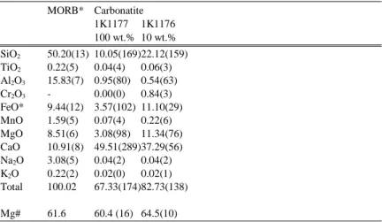
Experiments were performed on two series of chemical systems: (1) olivine–basalt systems and (2) olivine–carbonatite systems. The olivine–basalt systems were mixtures of powder made of the San Carlos olivine (Mg0.9,Fe0.1)2SiO4 with 1, 2, 3 and 10 wt.% of basalt. The source of the basalt was natural mid-ocean ridge basalt (SUNY MORB: Richter et al., 2003). The olivine–carbonatite systems were mixtures of powder made of the San Carlos olivine with 1, 3, 10 and 100 wt.% of carbonatite from Phalaborwa, South Africa. The size of powder of San Carlos olivine was a few µm in diameter. The chemical compositions of the starting melt sources are shown in Table 1.
In situ electrical conductivity measurements were performed using a Kawai-type multi-anvil
apparatus. Tungsten carbide was used as second stage anvils encasing an octahedral pressure cell. The pressure cell was composed of MgO and Cr2O3, and had edge lengths of 25 mm and truncated lengths of 15 mm. Heating was accomplished using a graphite furnace contained in the octahedral pressure medium. The powdered sample was encapsuled in a cylindrical MgO sample sleeve and was closed on each end by a graphite electrode that was in contact with two sets of W97Re3–W75Re25 thermocouples. Graphite disk electrodes with a diameter of 2 mm were placed in contact with a sample so that oxygen fugacity was controlled on the C–CO buffer. Two sets of thermocouples were mechanically connected to each graphite electrode on the sample and were insulated from the graphite furnace by Al2O3 and MgO insulators. These were also used for the four-wire resistance method of electrical conductivity measurement. The design of cell assembly is shown in Fig. 1.
Impedance spectroscopic measurements were carried out using a Solartron 1260 impedance Gain-Phase Analyzer combined with a Solartron 1296 interface, which makes it possible to measure a very high impedance material (up to 1014 ohm). Complex impedances were obtained at frequencies ranging from 1 MHz to 1 Hz. The fundamental applied voltage is 1.41 V. The impedance spectra generally show one arc at high frequencies and an additional part appears at low frequencies (Fig. 2). To distinguish between grain boundary transport and electrode process in the impedance spectrum, complex impedances were measured from 1 MHz to 1 mHz for one experiment of the olivine+basalt system (Fig. 2c). At low frequencies below 1 kHz, 45˚ of slope in the complex impedance plane represents a Warburg diffusion impedance. If melt phase is interconnected in a solid matrix, it forms an electrical pathway in parallel with the solid matrix (Roberts and Tyburczy, 2000). Thus the high-frequency arc reflects the sample properties, and the low frequency tail is accordingly interpreted as an effect of the electrodes. Therefore, only the first arc was used to determine the sample conductivity. At low temperatures, only the first arc appears. In this case, an equivalent circuit was composed of a sample resistance and capacitance in parallel and was fit to the experimental data for the determination of sample resistance. At high temperatures, it is difficult to define the first arc, because measurement in a range of much higher frequencies (higher than 1 MHz) is required to observe the first arc. In this situation, conductivity values were computed from impedance values Z′ taken at the frequency where the phase shift is closest to zero.
Conductivity measurements of the olivine–basalt system and the carbonate-bearing systems were conducted at 1.5 GPa and 3 GPa, respectively. Several heating–cooling cycles were carried out. The temperature was increased and decreased with steps of 25–50 K up to the
desired temperature. Impedance spectroscopy was conducted at each step. In the first cycle, the sample was heated to 1000 K, and then cooled to 800 K after annealing for several hours to dehydrate the sample and the surrounding materials, and to close cracks and pores by sintering. The conductivity usually decreased during pre-annealing at 1000 K. In the second cycle, the sample was heated to the desired temperature which is above the liquidus of the melt components. To acheive textural equilibration of the solid–liquid composites, the olivine–basalt systems were annealed for a few hours at 1600 K which is above the liquidus temperature of MORB at 1.5 GPa. For the olivine– carbonatite system, the annealing temperature to establish the textural equlibrium was 1650 K or 1700 K at 3 GPa. After annealing, the sample was cooled to 800 K. Subsequent heating cycles using step-wise temperature increments were also conducted to confirm reversibility. Time scale for each measurement was approximately 3 min. For measurements during cooling, a confirmation of establishment of steady state was not performed. However, measurements at lower T were rather stable with time because texture was quenched. Average cooling rate including measurement time was around 10 K per minute. In order to hold the partial molten texture, the sample was quenched from the highest temperature to ambient temperature. To obtain information on the melt conductivity, the conductivity of the carbonatite was also measured independently from the partial molten samples.
Fig. 3 shows the conductivity variation with time. The conductivity fluctuated during the first a few minutes at the maximum annealing temperature and then became nearly constant after 1 h annealing at the maximum temperature. Continuous monitoring of electrical conductivity at constant temperature permits evaluation of the rate of textural equilibrium where the interfacial energy of the system reaches its minimum. The above dependence of conductivity with time implies that the samples reached textural equilibirum. After the establishment of the textural equilibration, the partial-melt geometry is likely to keep self-similarity even if grain growth occurs. Thus the bulk conductivity could not change with time due to the grain growth.
Retrieved samples were mounted in epoxy and ground parallel to the long axis of heater. The chemical compositions of carbonate and silicate phases in the recovered sample were obtained by electron microprobe analysis. Representative chemical compositions of carbonatitic melt in run products are shown in Table 1. Microscopic observations were made using secondary electron (SEI) and backscattered electron images (BEIs) by field-emission scanning electron microscope (FE-SEM). The melt fraction of the samples was determined by image analysis after the experiments followed by the method of Yoshino et al. (2005). To separate the melt phase from crystal, the gray scale BEI images were converted to binary images. Then, binary images were treated by NIH image software to determine melt area. At least 5 BEI images were used to determine the melt volume fraction.
There were slight differences in the melt fraction and composition expected from the preparation of the samples in association with a change of bulk composition of the system. However, the melt conductivity is not sensitive to small changes in the melt composition, because the diffusion coefficients of the different elements in the melt are very similar (Kress and Ghiorso, 1993).
3. Experimental results
3.1. Olivine–basalt system
Fig. 4 shows the BEI on the polished surface of the recovered samples. Grain size of olivine crystals was around 10–20µm in diameter, suggesting that grain growth of olivine crystals occurred during the experimental runs. In order to characterize chemical interactions between the sample and components forming the conductivity cell, interfaces between the MgO sleeve
and graphite electrodes with the sample were carefully observed by FE-SEM (Fig. 4). Although iron diffused slightly into the MgO sample container (b10 µm), there was no infiltration of basaltic melt into the MgO capsule and no reaction product at the interface between MgO sleeve and the partial molten sample. The volume fractions estimated after conductivity measurements by image analysis were close to the ratio expected from the basalt and olivine mixed proportions. The estimated volume fractions of melt are 0.9, 2.4, 3.1 and 11% for the 1.0, 2.0, 3.0 and 10.0 melt weight fractions, respectively.
The olivine–basalt system shows relatively uniform melt distribution at low melt fraction. All of the triple junctions among three olivine grains contain melt (Fig. 4 a). This observation is consistent with previous studies on melt distribution in mantle rocks (e.g., Waff and Bulau, 1979). As the melt fraction increases, triple junction tubules along grain edges extend deeper into grain boundaries with increasing melt fraction (Fig. 4b). When the melt fraction is over 10%, the melt distribution becomes heterogeneous, and melts commonly surrounded by four or more grains are more common. As shown in Fig. 4c, the development of flat grain-melt interfaces (faceting) is more common for higher melt fraction sample. Since the faceted systems tend to produce more facet boundaries at the pore walls due to the difference of interfacial energies between the flat and curved surfaces, heterogeneity of melt distribution would be enhanced in the rocks with high melt fraction (Yoshino et al., 2006b).
An example of conductivity measurements along heating and cooling paths is shown in Fig. 5. In the first heating cycle to 1000 K, the measured conductivities were relatively high (N10−3 S/m). During annealing at 1000 K, conductivity generally decreased and became nearly constant after a few hours. At the same temperatures, the conductivity in the first cooling was lower than that in the first heating. In the second heating, a large increase in conductivity occurred at 1360 K, corresponding to the solidus of MORB composition. This temperature agrees with that reported in literature (e.g.; Yasuda et al., 1994). At 1600 K, above the MORB liquidus, the conductivity increased slightly during the first 3 min, and then achieved a final value during the remainder of the cycle. In the second cooling path, a large decrease in conductivity occurred at 1500 K corresponding to the MORB liquidus. In addition, a change of slope in the Arrhenius plot occurred at 1150 K. This may correspond to the crystallization of the basaltic melt (e.g. Burkhard, 2001). The conductivity continuously decreased to 3•10−4 S/m as the temperature decreased to 1000 K.
The conductivities at the temperature maxima are presented in Table 2. The conductivity obtained for the olivine–basalt system increased by one order of magnitude with increasing melt fraction from 0.9 to 11 vol.%. The conductivities of the olivine–basalt rocks and basaltic melt are by more than one order of magnitude higher than that of anhydrous olivine measured under the same conditions (Yoshino et al., 2006a).
3.2. Olivine–carbonatite system
Four experiments on the olivine–carbonatite system containing 1, 3, 10 and 100 wt.% carbonatite melt were performed up to at least 1650 K at 3 GPa. There was no infiltration of carbonatite melt into the MgO capsule. A diffusion distance (b10 µm) of iron into the surrounding MgO is similar to that of the olivine–basalt system. The melt fractions obtained after conductivity measurements were also close to those expected from the starting compositions (see Table 2). As shown in Fig. 4d–f, the melt distribution was homogeneous throughout the sample, even if the melt fraction is high (∼10%). The morphology of the small carbonatite melt pools is characterized by convex shapes showing small dihedral angles (b60˚). Compositional zoning of olivine crystals showing Fe depletion at the rim was observed. The Mg number in olivine increases from 90.8±0.2 to 94.2±0.7 with increasing melt fraction because of the preferential dissolution of Fe into the carbonatitic melt.
In the first cycle, the change of conductivity was small during annealing at 1000 K. In the second heating, a large increase of conductivity more than one order of magnitude occurred between 1000 and 1200 K. This temperature is consistent with the temperature at which the conductivity of Ca-rich carbonate abruptly increases during heating (e.g. Gaillard et al., 2008). Up to the desired maximum temperature, the conductivity increased linearly. The conductivity values firstly decreased and then became almost constant at the maximum temperature after annealing for 1 h (Fig. 3). In the second cooling path, the conductivity gently decreased to 900 K. An abrupt change of slope in the Arrhenius plot occurred at 900 K. This may correspond to the crystallization of the carbonatite. In the third heating, the conductivity value at the maximum annealing temperature was the same as that at the beginning of the second cooling. The absolute values during the third heating were slightly higher than the values of the second cooling path in a temperature range of 950–1400 K. This tendency was also observed for the other samples of the olivine–carbonatite system.
The conductivity obtained for the olivine–carbonatite system increased with increasing melt fraction (Fig. 6). The conductivity of carbonatitic melt was around 102 S/m at 1700 K, and abruptly decreased at 1625 K. This temperature corresponds to the melting temperatureof the carbonatite melt weused. Thecalculated activation enthalpy for electrical conduction in carbonatite melt is 0.38 eV, which is close to the values (0.31–0.35 eV) reported from Gaillard et al. (2008). The absolute conductivity value of the carbonatite melt was slightly lower than those reported by Gaillard et al. (2008), because melts commonly have a positive activation volume for electric conduction (Tyburczy and Waff, 1983) and the natural carbonatite we used contains a considerable amount of silicate component. The conductivities of the olivine–carbonatite system are nearly one order of magnitude higher than the olivine– basalt system at the same melt fraction, and are nearly two orders of magnitude higher than those of the olivine even if the melt fraction is ∼1 vol.% (e.g., Constable, 2006; Yoshino et al., 2006a).
4. Discussion
4.1. Archie's law
We demonstrated that both partial molten systems show higher conductivity than the system without melt. As shown in Fig. 5b, the temperature dependence of the conductivity for the olivine–basalt system suggests that the bulk conductivity is mainly controlled by the melt ,and that the melt is interconnected in the olivine matrix (Yoshino et al., 2003). In addition, the previous studies on melt textures suggested that the dihedral angle of the olivine–basalt system is generally around 30˚ (Waff and Bulau, 1979; Hirth and
Kohlstedt, 1995; Yoshino et al., 2005; 2009). Therefore, the basaltic melt forms three-dimensional interconnection in the olivine aggregate. For the olivine–carbonatite system, temperature dependence of the conductivity is not clearly identified. However, the carbonatite melt also has low dihedral angles of largely less than 60˚ (28˚: Hunter and McKenzie, 1989). Therefore, the high conductivities obtained from these two different systems compared to the olivine conductivities could be derived from the interconnection of partial melt in olivine aggregates.
This study demonstrates that each partially molten system with various melt fractions shows an increase of conductivity with increasing melt content. Fig. 7 shows log conductivity versus melt volume fraction for each system. The data for each system shows a linear relation in this plot. This behaviors can be represented by the Archie's law (Archie, 1942). Archie's relation is also an empirical equation that relates the electrical conductivity to the fraction of liquid phase as follows:
σbulk = CΦnσm (1)
where C and n are constants (e.g., Watanabe and Kurita, 1993). This relation is commonly applied to represent fluid connectivity in sandstones saturated with water. In this model, the conductivity of the solid phase is assumed to be negligibly small. The present data for each system can be fitted very well by Eq. (1). The fitting parameters for each system are shown in Table 3.
The constants C and n of the olivine–basalt systems show lower values (C =0.67, n =0.89) than those of the olivine–carbonatite system (C =0.97, n =1.14). These values are similar to those determined from the partial molten peridotite composed of Fo80 and MORB (C =0.73, n =0.98) (Roberts and Tyburczy, 2000). On the other hand, they are smaller than those determined from the forsterite with various content of melt in CaO–MgO–Al2O3–SiO2 system (C =1.47, n =1.30) (ten Grotenhuis et al., 2005). Watanabe and Kurita (1993) also determined the constants for a system consisting of ice and liquid KCl, which is an analogue for a partially molten peridotite system. For melt fractions less than 0.2, the calculated n values (1.34–1.74) are much higher than our system, and similar to the result of ten Grotenhuis et al. (2005). Watanabe and Kurita (1993) concluded that for their system Archie's law indicates a change from a relatively large portion of isolated pockets, at low melt fraction, to more melt in triple junction tubes, at high melt fraction. On the other hand, ten Grotenhuis et al. (2005) concluded that for their system Archie's law indicates a gradual change of melt distribution from triple junction tubes, at low melt fractions, to melt layers along grain boundaries, at high melt fractions. However, the low n values for our system suggest that such a change of melt distribution is not so large in a range of the measured melt fraction. The fact that the more realistic systems used by the present study and Roberts and Tyburczy (2000) show similar n values suggests that analogue systems are not suitable for understanding the melt distribution of partial molten peridotite.
4.2. Geometrical considerations of partial melt
Archie's law is not a geometrical model. It is just an empirical expression. To consider the 3-D melt morphology of the partial molten system, the conductivity-melt fraction relationships obtained from this study are compared with some theoretical predictions based on simple geometrical melt distributions. Temperature changes should cause drastic changes of melt composition and wetting properties. To avoid this complexity, we present conductivity-melt relations under isothermal conditions in this study.
There are various theoretical models for estimating the bulk conductivity of partially molten rocks from the conductivity of melt and solid phases. Waff (1974) proposed a simple model to describe the bulk conductivity as a function of melt fraction. This model assumes that cubic grains are surrounded by a melt layer with a uniform thickness dependent on melt fraction (Φ) and that the solid conductivity is negligibly small. The bulk conductivity (σbulk) is given by σbulk=[1−(1−Φ)2/3] σm (2)
where σm is the conductivity of melt.
A frequently used model to predict the maximum effective bulk conductivity of an interconnected two-phase mixture is Hashin and Shtrikman (HS) upper bound (Hashin and Shtrikmann, 1962). This upper bound is representative for melts distributed along grain boundaries and filling triple junctions of spherical grains. The upper bound of effective conductivity (σ) of a system can be defined as a function of melt fraction by the following equation;
where σm and σs are the conductivity of melt and solid, respectively. The opposite case representing the isolated spheres of melt in solid grains is known as the HS lower bound. The model focusing on triple junction tubes filled with melt is the tube model by Schmeling (1986). In this model the melt is distributed in equally spaced tubes within a rectangular network. The effective conductivity is given by
Fig. 8a shows the measured bulk conductivity versus measured melt volume fraction together with various mixing models for the olivine– basalt system. For the olivine–basalt system, we consider 1600 K, which is the annealing temperature applied to achieve textural equilibrium in this study. Basaltic melt conductivity is fixed at 10 S/m, based on the results given by Presnall et al. (1972). Olivine conductivity is fixed at 10−2.2 S/m, based on the Constable (2006). The cube-type (Waff, 1974) or sphere-type models (Hashin and Shtrikmann, 1962) explain the present experimental results well. This suggests that the conducting melt fully wets the grain boundaries of the less conductive olivine matrix composed of cubic or spherical grains. However, the sample with the maximum melt fraction (11 vol.%) shows slightly lower conductivity in comparison with the HS upper bound. The development of faceting occasionally leads to a remarkably inhomogeneous melt distribution (Yoshino et al., 2006b). The textural observation shows the development of large pools surrounded by four or more grains and the corresponding shrinkage of triple junctions at high melt fraction. The large melt pockets are isolated and connected by thin melt film. Since large melt pockets surrounded by four or more grains contain a significant fraction of the total melt fraction, the bulk conductivity of an olivine–basalt system with high melt fractions would be lower than that predicted from the HS upper bound.
Fig. 8b shows the case for the olivine–carbonatite system at 1650 K, which is just above the liquidus of carbonatite we used. Carbonatite melt conductivity is fixed at 102 S/m based on our result. Olivine conductivity is fixed at 10−2.1 S/m based on the Constable (2006). The present data are also fitted very well by cube-type or sphere-type (HS upper bound) models (Waff, 1974; Hashin and Shtrikmann, 1962). They are more consistent with these models than those of the olivine–basalt system, especially for high melt fractions N10%. They are also consistent with homogeneous melt distribution independent of the melt fraction observed by textural analysis.
ten Grotenhuis et al. (2005) proposed that the melt distribution gradually changes from triple junction tubes to melt layers along grain boundaries. Although the present study can not confirm such a systematic change of melt distribution for both the olivine–basalt and the olivine–carbonatite systems by electrical conductivity measurement, textural observation suggests that a triple junction network is dominant at low melt fractions. If the melt fraction is proportional to the thickness of melt layer along the grain boundary, the constant n should be around 2/3. Constants n higher than 2/3 should indicate that the melt distribution gradually changes from triple junction tubes to melt layers along grain boundaries as the melt fraction increases.
4.3. Permeability of partial molten rocks
ridges. Magmatic melts rise through the partially molten region as a form of permeable flow. The permeability (k) is an essential parameter for estimating the rate at which melt can be expelled from the melt source region. An empirical permeabilitymelt fraction relation, Kozney–Carman permeability (Carman, 1956), has been widely used to estimate the permeability of various kinds of porous materials. This relation can predict the permeability above 20% liquid fraction, whereas permeability is significantly reduced at low liquid fraction (Riley and Kohlstedt, 1991; Wark and Watson, 1998). The permeability is controlled not only by the melt fraction but also by connectivity and melt morphology as well as electrical conduction. Katz and Thompson (1987) presented a model that predicts permeability from electrical conductivity measurement. Takashima and Kurita (2008) also proposed a power relationship (power exponent is 2) between permeability and electrical conductivity based on permeability and electrical conductivity measurements using gel as an analogue of the solid phase of the partially molten system. Thus, the electrical conductivity-melt fraction relationship is useful for estimating the permeability at low melt fraction (less than 20%). Faul et al. (1994) suggested that melt distributions consist of small proportions (b15%) of triple junction tubes and large proportions of disk-shaped layers on two grain boundaries because of faceting of olivine crystals in partial molten rock. Based on observations of the size differences between triple junction geometries and melt pools surrounded by more than 4 grains for the olivine–basalt system, Faul et al. (1997) proposed a porosity–permeability model that predicts permeability of partial molten peridotite. In this model, permeability sharply increases about 4 orders of magnitude at 2% melt fraction because of the percolation of disk-shaped melt layers. Our results show no evidence of such a sharp increase of conductivity above melt fractions of at least 1%. Wark et al. (2003) showed that 2-D slices through the pore network may appear “disk-shaped” as melt fraction increases, when in fact the pore network is composed of triple junction tubules. Furthermore, the pore geometry for the olivine– basalt system is well approximated by a triple junction tube network, based on the relationship between grain boundary wetness (contiguity) and melt fraction (Yoshino et al., 2005). In fact, Wark and Watson (1998) predicted a gradual increase of permeability with increasing porosity based on permeability measurements for quartz– fluid system at low porosity (0.006–0.17). Therefore, we conclude that permeability of partial molten peridotites gradually increases with increasing melt fraction without the percolation threshold as well as those predicted from the ideal model. For the olivine–basalt system, as melt fraction increases, the permeability would be lower than that estimated from the ideal model by the development of large melt pool.
It is well known that carbonatite melt is several orders of magnitude more mobile than basaltic melt in an olivine matrix (e.g., Minarik and Watson, 1995; Hammouda and Laporte, 2000). If our data are normalized by the melt conductivity, the conductivity-melt fraction relationship of carbonatite melt is similar to that of basaltic melt. The permeability of partial molten rocks is only controlled by melt morphology in solid crystals as a function of melt fraction. In fact, Takashima and Kurita (2008) found that the permeability is proportional to the square of the electrical conductivity. If these melts migrate by porous flow, a difference of migration distance between carbonatite and basaltic melts is not controlled by the permeability. Therefore, fast migration of carbonatite melt would be mainly controlled by lower viscosity than basaltic melt due to fast diffusion of carbonate components in the melt.
4.4. Estimation of melt fraction in the upper mantle
Archie's relation obtained from this study can be used to deduce melt fractions in the partially molten region in the upper mantle from electromagnetic studies. Jegen and Edwards (1998) estimated 0.2– 0.6 S/m for the conductive zone beneath the Juan de Fuca mid-ocean ridge based on the electromagnetic sounding survey. Evans et al. (2005) reported a conductivity
anomaly with strong anisotropy below 60 km depth near mid-ocean ridge of the Eastern Pacific Rise. In this region, the highest conductivity value is around 0.1 S/m. As Shankland and Waff (1977) suggested, anomolously high conductivity at shallow mantle depth has been regarded as 0.1 S/m. We will use this value (0.1 S/m) as a reference to estimate typical melt fractions of the region showing high conductive anomaly in the upper mantle.
Firstly we consider the case of the basaltic melt. Because the basaltic melt has a relatively large temperature dependence (Presnall et al., 1972), it is necessary to consider the effect of temperature on the conductivity values of partial molten rocks. As shown in Fig. 9,we also constructed Archie's relationship for the olivine–basalt system based on our conductivity measurements at 1500 K, which is just above the basalt liquidus at 1.5 GPa. The melt fractions required to explain the conductivity of 0.1 S/m are 1 and 3 vol.% at 1600 and 1500 K, respectively. This range of melt fractions is consistent with the minimum melt concentration of 1 to 2 vol.% in the melt production region predicted from shear wave delays and Rayleigh wave velocity variations (The MELT seismic team, 1998).
Next we consider carbonatite melt, which is only stable above 2.5 GPa (Dalton and Presnall, 1998), as a conductive agent in the upper mantle. As the temperature dependence of conductivity on carbonatite melt is small (Gaillard et al., 2008), the conductivity was assumed to be constant as a function of temperature. As shown in Fig. 9, the estimated melt fraction of carbonatite is approximately 0.3 vol.%, which is one third to one order of magnitude lower than that for basaltic melt (1 to 3 vol.%), and slightly higher than that (0.1 vol.%) predicted from Gaillard et al. (2008), who firstly argued that the enhanced electrical conductivity of the low velocity zone (LVZ) beneath oceanic lithsphere is owing to small amounts of carbonatite melt. Hirschmann (2010) recently claimed that carbonatite cannot be present in large regions of the LVZ at intermediate depths (60– 145 km) based on the petrological constraints assuming the representative volatile content (100 ppm H2O, 60 ppm CO2). If the conductivity anomaly just beneath the oceanic lithosphere is caused by carbonatite melt, fast percolation of carbonatite melt derived from deeper magma is required to collect the melt at that depth. Dasgupta and Hirschmann (2006) experimentally demonstrated that the solidus temperature of carbonated peridotite from 3 to 10 GPa is below the mantle adiabat geotherm. Its low solidus temperature can produce the conductivity anomaly in the regions shallower than 330 km depth. Hirschmann (2010) suggested that carbonatite melt can be stable below depths of 130–180 km for the mantle peridotite contaning typical amounts of volatile components. They proposed that melting beneath the mid-ocean ridge occurs depths up to 330 km, producing 0.03–0.3 wt.% carbonatite liquid. Our estimated melt fraction falls in this range. The deep electrical conductivity profile, obtained from analysis of data from a submarine cable extending from Hawaii to North America, showed a conductivity peak of 10−1 S/m at the depth range of 200–250 km (Lizarralde et al., 1995). Such a conductive anomaly can be explained by a presence of very small amount of carbonatite melt.
The carbonate content in partial melt of the carbonate-bearing peridotite decreases with increasing temperature, in other words, with increasing melt fraction (Dasgupta et al., 2007). As carbonate content in the partial melt decreases, the melt conductivity would change from that of carbonate melt to that of a silicate melt. At high melt fractions, the resulting bulk conductivity, therefore, may be much lower than our estimate. The effects of carbonatite melt in carbonate-bearing peridotite on the electrical conductivity of the upper mantle will be discussed elsewhere (Yoshino et al., in preparation).
5. Conclusions
In this study, distributions of basalt and carbonatite melts in olivine aggregates were investigated by means of in situ electrical conductivity measurement at high pressures, corresponding to the upper mantle. The Mg–carbonatite melt has one order of magnitude
higher conductivity than basaltic melt. Carbonatite melt-bearing rocks also show higher conductivity than basaltic melt-bearing ones for the similar melt fractions. The electrical conductivity data for each partially molten system with various melt fractions show an increase of conductivity with increasing melt content. For both systems, the electrical conductivity of the partially molten samples is best described by Archie's law (σbulk/σmelt = CΦn) with parameters C =0.68 and 0.97 and n =0.87 and 1.14 for the olivine–basalt and olivine–carbonatite systems, respectively. Comparing our electrical conductivity data with the predictions of geometric models for melt distribution, the model that melt forms layers along grain boundaries is the most likely for the range of melt fractions measured. The gradual change in conductivity with melt fraction suggests no permeability jump due to the melt percolation at a certain melt fraction. Melt fractions of 1–3 vol.% for basaltic melt or 0.3 vol.% for carbonatitic melt are sufficient to explain the high conductivity anomaly observed in the upper mantle.
Acknowledgments
We are grateful to E. Ito, D. Yamazaki, A. Yoneda, and D. Fraser for the discussions. The authors thank two anonymous reviewers for helpful comments. This work was supported by grant-in-aids for scientific research, no. 20340120 to TY from the Japan Society for Promotion of Science. It was also supported by the internship program (MISIP09) of the Institute for Study of the Earth's Interior, Okayama University.
References
Archie, G.E., 1942. Electrical resistivity log as an aid determining some reservoir characteristics. Trans. Am. Inst. Min. Metall. Pet. Eng. 146, 54–62.
Baba, K., Chave, A.D., Evans, R.L., Hirth, G., Mackie, R.L., 2006. Mantle dynamics beneath the East Pacific Rise at 17 S: insights from the Mantle Electromagnetic and Tomography (MELT) experiment. J. Geophys. Res. 111, B02101. doi:10.1029/2004JB003598.
Burkhard, D.J., 2001. Crystallization and oxidation of Kilauea basalt glass: process during reheating experiments. J. Petrol. 42, 507–527.
Carman, P.Z., 1956. Flow of Gases through Porous Media. Butterworths Sci. Publ, London. Constable, S., 2006. SEO3: a new model of electrical conductivity. Geophys. J. Int. 166, 435–437.
Dalton, J.A., Presnall, D.C., 1998. Carbonatitic melts along the solidus of model lhelzolite in the system CaO– MgO–Al2O3–SiO2–CO2 from 3 to 7 GPa. Contrib. Mineral. Petrol. 131, 123–135.
Dasgupta, R., Hirschmann, M.M., 2006. Melting in the Earth's deep upper mantle caused by carbon dioxide. Nature 440, 659–662.
Dasgupta, R., Hirschmann, M.M., Smith, N.D., 2007. Partial melting experiments of peridotite + CO2 at 3 GPa and genesis of alkalic ocean island basalts. J. Petrol. 48,2093–2124.
Evans, R.L., Hirth, G., Baba, K., Forsyth, D., Chave, A., Mackie, R., 2005. Geophysical evidence from the MELT area for compositional controls on oceanic plates. Nature 437, 249–252.
Faul, U.H., 1997. Permeability of partially molten upper mantle rocks from experiments and percolation theory. J. Geophys. Res. 102, 10,299–10,311.
Faul, U.H., Toomey, D.R., Waff, H.S., 1994. Intergranular basaltic melt is distributed in thin, elongated inclusions. Geophys. Res. Lett. 21, 29–32.
Gaillard, F., Marki, M., Iacono-Marziano, G., Pichavant, M., Scaillet, B., 2008. Carbonatite melts and electrical conductivity in the asthenosphere. Science 322, 1363–1365.
Hammouda, T., Laporte, D., 2000. Ultrafast mantle impregnation by carbonatite melt. Geology 28, 283–285. Hashin, Z., Shtrikmann, S., 1962. A variational approach to the theory of the effective magnetic permeability of
multiphase materials. J. Appl. Phys. 33, 3125–3131.
Hirano, N., Takahashi, E., Yamamoto, J., Abe, N., Ingle, S.P., Kaneoka, I., Kimura, J., Hirata, T., Ishii, T., Ogawa, Y., Machida, S., Suyehiro, K., 2006. Volcanism in response to plate flexure. Science 313, 1426–1428. Hirschmann, M.M., 2010. Partial melt in the oceanic low velocity zone. Phys. Earth Planet. Int. 179, 60–71. Hirth, G., Kohlstedt, D.L., 1995. Experimental constraints on the dynamics of the partially molten upper mantle:
Deformation in the diffusion creep regime. J. Geophys. Res. 100, 1981–2001.
Hunter, R.H., McKenzie, D., 1989. The equilibrium geometry of carbonate melts in rocks of mantle composition. Earth Planet. Sci. Lett. 92, 347–356.
Jegen, M., Edwards, R.N., 1998. Electrical properties of a 2D conductive zone under the Juan de Fuca ridge. Geophys. Res. Lett. 25, 3647–3650.
Katz, A.J., Thompson, A.H., 1987. Prediction of rock electrical conductivity from mercury injection measurement. J. Geophys. Res. 92, 599–607.
Kawakatsu, H., Kumar, P., Takei, Y., Shinohara, M., Kanazawa, T., Araki, E., Suyehiro, K., 2009. Seismic evidence for sharp lithosphere–asthenosphere boundaries of oceanic plates. Science 324, 499–502.
Kress, V.C., Ghiorso, M.S., 1993. Multicomponent diffusion in the MgO–Al2O3–SiO2 and CaO–MgO–Al2O3– SiO2 systems. Geochim. Cosmochim. Acta 57, 4453–4466.
Lizarralde, D., Chave, A.D., Hirth, G., Schultz, A., 1995. A Northern Pacific mantle conductivity profile from long-period magnetotelluric sounding using Hawaii to California submarine cable data. J. Geophys. Res. 100, 17,837–17,854.
Minarik, W.G., Watson, E.B., 1995. Interconnectivity of carbonate melt at low melt fraction. Earth Planet. Sci. Lett. 133, 423–437.
Presnall, D.C., Simmons, C.L., Porath, H., 1972. Change of electrical conductivity of a synthetic basalt during melting. J. Geophys. Res. 77, 5665–5672.
Richter, F.M., Davis, A.M., DePaolo, D.J., Watson, E.B., 2003. Isotope fractionation by chemical diffusion between basalt and rhyolite. Geochim. Cosmochim. Acta 67, 3905–3923.
Riley, G.N., Kohlstedt, D.L., 1991. Kinetics of melt segregation in upper mantle-type rocks. Earth Planet. Sci. Lett. 105, 500–521.
Roberts, J.J., Tyburczy, J.A., 2000. Partial-melt conductivity: influence of melt composition. J. Geophys. Res. 104, 7055–7065.
Schmeling, H., 1986. Numerical modelings on the influence of partial melt on elastic, anelastic and electric properties of rocks. Part II: electrical conductivity. Phys. Earth Planet. Int. 43, 123–136.
Shankland, T.J., Waff, H.S., 1977. Partial melting and electrical conductivity anomalies in the upper mantle. J. Geophys. Res. 82, 5409–5417.
Takashima, S., Kurita, K., 2008. Permeability of granular aggregate of soft gel: application to the partial molten system. Earth Planet. Sci. Lett. 267, 83–92.
ten Grotenhuis, S.M., Drury, M.R., Spiers, C.J., Peach, C.J., 2005. Melt distribution in olivine rocks based on electrical conductivity measurement. J. Geophys. Res. 110, B12201. doi:10.1029/2004JB003462.
The MELT seismic team, 1998. Imaging the deep seismic structure beneath a mid-ocean ridge: the MELT experiment. Science 280, 1215–1218.
Tyburczy, J.A., Waff, H.S., 1983. Electrical conductivity of molten basalt and andesite to 25 kilobars pressure: geophysical significance and implications for charge transport and melt structure. J. Geophys. Res. 88, 2413– 2430.
von Bargen, N., Waff, H.S., Waff, H.S., 1986. Permeabilities, interfacial areas and curvatures of partially molten systems: Results of numerical computations of equilibrium microstructures. J. Geophys. Res. 91, 9261–9276. Waff, H.S., 1974. Theoretical considerations of electrical conductivity in a partially molten mantle and
implications for geothermometry. J. Geophys. Res. 79, 4003–4010.
Waff, H.S., Bulau, J.R., 1979. Equilibrium fluid distribution in an ultramafic partial melt under hydrostatic stress condition. J. Geophys. Res. 84, 6109–6114.
Wark, D.A., Watson, E.B., 1998. Grain-scale permeabilities of texturally equilibrated, monomineralic rocks. Earth Planet. Sci. Lett. 164, 591–605.
Wark, D.A., Williams, C.A., Watson, E.B., Price, J.D., 2003. Reassessment of pore shapes in microstructurally equilibrated rocks, with implications for permeability of the upper mantle. J. Geophys. Res. 108, 2050. doi:10.1029/2001JB001575.
Watanabe, T., Kurita, K., 1993. The relationship between electrical conductivity and melt fraction in a partially molten simple system. Phys. Earth Planet. Int. 78, 9–17.
Yasuda, A., Fujii, T., Kurita, K., 1994. Melting phase relations of an anhydrous mid-ocean ridge basalt from 3 to 20 GPa: implications for the behavior of subducted oceanic crust in the mantle. J. Geophys. Res. 99, 9401– 9414.
Yoshino, T., Walter, M.J., Katsura, T., 2003. Core formation in planetesimals triggered by permeable flow. Nature 422, 154–157.
Yoshino, T., Takei, Y., Wark, D.A., Watson, E.B., 2005. Grain boundary wetness of texturally equilibrated rocks, with implications for seismic properties of the upper mantle. J. Geophys. Res. 110, B08205. doi:10.1029/2004JB003544.
Yoshino, T., Matsuzaki, T., Yamashita, S., Katsura, T., 2006a. Hydrous olivine unable to account for conductivity anomaly at the top of the asthenosphere. Nature 443, 973–976.
Yoshino, T., Price, J.D., Wark, D.A., Watson, E.B., 2006b. Effect of faceting on pore geometry in texturally equilibrated rocks: implications for low permeability at low porosity. Contrib. Mineral. Petrol. 152, 169–186. Yoshino, T., Yamazaki, D., Mibe, K., 2009. Well-wetted olivine grain boundaries in partial molten peridotites in
the asthenosphere. Earth Planet. Sci. Lett. 283, 167–173.
Yoshino, T., Laumonier, M., MacIsaac, E., Katsura, T., Effect of carbonate content on electrical conductivity of partial molten carbonate peridotites. in preparation.
Table 1. Melt composition of starting materials and run products MORB* Carbonatite 1K1177 1K1176 100 wt.% 10 wt.% SiO2 50.20(13) 10.05(169) 22.12(159) TiO2 0.22(5) 0.04(4) 0.06(3) Al2O3 15.83(7) 0.95(80) 0.54(63) Cr2O3 - 0.00(0) 0.84(3) FeO* 9.44(12) 3.57(102) 11.10(29) MnO 1.59(5) 0.07(4) 0.22(6) MgO 8.51(6) 3.08(98) 11.34(76) CaO 10.91(8) 49.51(289) 37.29(56) Na2O 3.08(5) 0.04(2) 0.04(2) K2O 0.22(2) 0.02(0) 0.02(1) Total 100.02 67.33(174) 82.73(138) Mg# 61.6 60.4 (16) 64.5(10)
*Chemical composition of SUNY MORB was determined by EDS (Richter et al., 2003).
The chemical compositions of majorite were measured by the electron probe microanalyzer under the operating condition of 15 kV and 12 nA. Mg# is calculated from Mg/(Mg+Fe).
Table 2. Summary of runs
Run No. wt.% a vol.%b T
max (K) logmax (S/m) Remarks
Olivine + basalt 1K1154 1 0.9 1600 -1.00 No 2nd cooling path 1K1152 3 3.2 1600 -0.38 1K1156 10 10.3 1600 -0.09 Olivine + carbonatite 1K1166 1 0.7 1650 -0.49 1K1169 3 2.9 1650 0.29 1K1176 10 10.0 1700 0.76 c 1K1177 100 100 1700 1.95 c
a: Weight percent of basalt, carbonatite and dolomite in starting materials. b: Volume percent of melt phase in run products determined by image analysis. c: Log conductivity measured at 1650 K.
Table 3. Parameter values fitted by Eq (1)
Analyzed system C n R2 Reference olivine-basalt 0.68 0.87 0.98 this study
olivine-carbonatite 0.97 1.14 0.99 this study
Ice-KCl 0.02-0.30 1.34-1.74 Watanabe & Kurita (1993) Fo80(95)-MORB(5) 0.73 0.98 Roberts & Tyburczy (1999)
Figure Caption
Fig. 1. Schematic cross-section of high-pressure cell assembly for conductivity measurements in the Kawai-type multi-anvil press. Two sets of thermocouple connected to the graphite electrodes have an electric circuit similar to the 4-wire resistance method. Electrodes for heater are connected by Mo foil to the tungsten carbide cube.
Fig. 2. Complex impedance spectra showing the semicircular pattern of the real vs. imaginary components of complex impedance at frequencies ranging from 1MHz to 0.1 Hz at the temperatures indicated. (a) Impedance spectra of the carbonatite melt. (b) Impedance spectra of the olivine-carbonatite melt (10 wt.%).
Fig. 3. Back-scattered electron images of polished samples. The darker and brighter portions indicate olivine and melt phase, respectively. The olivine aggregates with different proportion of basaltic melt (a-c) and carbonatite melt (d-f). (a) An image of a sample with the lowest proportion of basaltic melt (~1 vol. %). Most of melts are located at triple junction of olivine crystals. (b) An image of sample with ~3 vol. % basaltic melt. Grain boundaries are largely covered with basaltic melt. (c) A sample with ~10 vol.% basaltic melt. Note that distribution of basaltic melt is relatively heterogeneous. (d) An image of a sample with the lowest proportion of carbonatite melt (~0.7 vol. %). Most of melts are located at triple junction of olivine crystals. (e) An image of a sample with ~3 vol.% carbonatite melt. (f) An image of sample with ~10 vol. % carbonatitic melt. Some parts filled with carbonatite melt were lost during polishing.
Fig. 4. Electrical conductivity of the olivine-basalt system as a function of reciprocal temperature. (a) Electrical conductivity of the olivine with 3 wt.% basalt as a function of reciprocal temperature during the heating-cooling cycles. Lines and dashed lines indicate heating and cooling cycles, respectively. (b) Electrical conductivity data of all samples in the Arrhenius plot. The symbols indicate raw data of cooling path after annealing at 1600 K for each sample with different melt fraction. The sample with 1 wt.% basalt could not obtain the cooling path after annealing because short circuit occurred during annealing. Abbreviations; TW83: conductivity data of tholeiitic melt at 0.1 MPa from Tyburczy and Waff (1983). PSP73: basalt electrical conductivity at 0.1 MPa from Presnall et al. (1973).
Fig. 5. Electrical conductivity of the olivine-carbonatite system as a function of reciprocal temperature. (a) Electrical conductivity of the olivine with 3 wt.% carbonatite as a function of reciprocal temperature during the heating-cooling cycles. Lines and dashed lines indicate heating and cooling cycles, respectively. (b) Electrical conductivity data of all samples in the Arrhenius plot. The symbols indicate raw data of cooling path after annealing at the maximum temperature for each sample with different melt fraction. Shaded area denotes the conductivity range of Mg-free carbonatite with various compositions at 0.1 MPa (Gaillard et al., 2008). Abbreviations; C06: the latest model of olivine electrical conductivity at 0.1 MPa under IW (iron-wüstite) buffers from Constable (2006). YMYK06: A conductivity range of electrical conductivity of olivine single crystal at 3 GPa under Ni-NiO buffer from Yoshino et al. (2006a).
Fig. 6. Relation between the melt fraction and electrical conductivity of the partial molten peridotites. The solid lines indicate the fitting results obtained from Eq. (1).
Fig. 7. Experimental data on bulk electrical conductivity of the partially molten samples plotted as a function of the melt fraction (solid circles). Curves represent the several mixing model predicted by inserting the measured melt conductivity into the melt distribution models. (a) Olivine-basalt system at 1600 K. Input data for the melt distribution models and conductivity of the basaltic melt (101 S/m) and olivine (10-2.2 S/m) are also presented. (b) Olivine-carbonatite system at 1650 K. Input data for the melt distribution models and conductivity of the
carbonatite melt (101.95 S/m) and olivine (10-2.1 S/m) are also presented.
Fig. 8. Relation between the melt fraction and electrical conductivity for the basalt and carbonatite melt-bearing peridotite. A plot of the olivine plus basalt 1 wt.% at 1500 K is estimated from the difference of conductivity for the sample consisting of olivine plus bsasalt 3 wt.% between 1500 and 1600 K. Shaded region indicates a typical range of conductivity values observed in regions with high conductive anomaly of the upper mantle (reference in the text).
5mm MgO Cr-doped MgO MgO Graphite ZrO2 Al2O3 Sample Thermocouple Thermocouple Mo
-2500 -2000 -1500 -1000 -500 0 -500 0 500 1000 1500 2000 2500 1K1177 Carbonatite
Z
''(
b
)
Z'(a)
1250 K 1300 K 1350 K 1400 K 1450 K 1500 K -30 -20 -10 0 10 -10 0 10 20 30 Z ''( b ) Z'(a) 1600 K 1650 K -2500 -2000 -1500 -1000 -500 0 500 -500 0 500 1000 1500 2000 2500 3000Z
''(
b
)
Z'(a)
1K1176 Olivine + Carbonatite 10 wt.% 1300 K 1350 K 1400 K 1450 K 1500 K 1600 K 1700 K(a)
(b)
(a)
Ol+ basalt 1 wt.%
(e)
Ol+ carbonatite 3 wt.%
(f)
Ol+ carbonatite 10 wt.%
(b)
Ol+ basalt 3 wt.%
(c)
Ol+ basalt 10 wt.%
(d)
Ol+ carbonatite 1 wt.%
Ol + BS 10 wt.%
Ol + BS 3 wt.%
Olivine + Basaltic melt
L
o
g
[C
o
n
d
u
c
ti
v
it
y
(S
/m
)]
-2 -1.5 -1 -0.5 0 0.5 1 1.5 0.6 0.65 0.7 0.75Basa
ltic m
elt (
PS
P7
3)
Thole
iite m
elt (T
W83
)
1000/T
-6 -5 -4 -3 -2 -1 0 1 0.6 0.8 1 1.2 1.4 1st H 1st C 2nd HL
o
g
[C
o
n
d
u
c
ti
v
it
y
(S
/m
)]
1000/T
2nd C1K1152
Olivine + basalt 3 wt.%
glass transition MORB solidus MORB liquidus(a)
(b)
Ol + BS 1 wt.%-4 -3 -2 -1 0 1 2 3 0.5 0.6 0.7 0.8 0.9 1 1.1 1.2 1.3 100 wt.% 10 wt.% 3 wt.% 1 wt.% carbonatite (GMIPS08)
L
o
g
[C
o
n
d
u
c
ti
v
it
y
(S
/m
)]
1000/T
Olivine + Carbonate melt
C
06
o
l
YM
YK
06
-4 -3 -2 -1 0 1 0.6 0.7 0.8 0.9 1 1.1 1.2 1.31K1169
Olivine + Carbonatite 3 wt.%
L
o
g
[C
o
n
d
u
c
ti
v
it
y
(S
/m
)]
1000/T
1st H 1st C 2nd H 2nd C 3rd H(a)
(b)
n
=
1.
14
n =
0.8
7
0.01
0.1
1
10
100
0.001
0.01
0.1
1
carbonatite basaltL
o
g
[C
o
n
d
u
c
ti
v
it
y
(S
/m
)]
Melt fraction
-2.5 -2 -1.5 -1 -0.5 0 0.5 1 1.5 0 0.05 0.1 0.15