Developing biophysical markers for anemic disorders through advancing interferometric microscopy

Developing Biophysical Markers for Anemic Disorders

through Advancing Interferometric Microscopy

by Poorya Hosseini

M.Eng., McGill University (2011)

B.Sc., Iran University of Science and Technology (2008)

Submitted to the Department of Mechanical Engineering in Partial Fulfillment of the Requirements for the Degree of

Doctor of Philosophy at the

MASSACHUSETTS INSTITUTE OF TECHNOLOGY

September 2017

C

Signature of Author ...

Certified by ...

Accepted by...

Signature redacted

Signature redacted

August 22, 2017

Peter T.C. So Professor of Mechanical and Biological Engineering

Thesis Supervisor

Signature

reaactea

Rohan Abeyaratne Chairman, Department Committee on Graduate Thesis, MIT

MASSANORSETTS INSTITUTE

QF TEPHNPLOGY

SEP

2 2 2017

LIBRARIES

Developing Biophysical Markers for Anemic Disorders

through Advancing Interferometric Microscopy

by

Poorya Hosseini

Submitted to the Department of Mechanical Engineering on August 2 2"d 2017

in Partial Fulfillment of the Requirements for the Degree of Doctorate of Philosophy in Mechanical Engineering

Erythrocytes, better known as red blood cells, among various functions, are mainly tasked with the oxygen transport in vertebrates through blood circulation. Red blood cells are packed with the hemoglobin, an oxygen-binding molecule, and have unique biophysical properties that are critical in enabling the oxygen delivery and optimization of the blood flow in large vessels and capillaries. These properties such as cellular deformability, biconcave shape, and proper hemoglobin function are compromised in a range of diseases known as anemic disorders. Quantifying these alterations provides a tool for studying pathobiology of these diseases and guides the search for the cure or novel treatments. Interferometric microscopy in various forms has been suggested as a tool for measuring some of these biophysical properties. However, current interferometric techniques suffer from one or a combination of the following shortcomings: (1) precision of the biophysical measurements is limited due to limits on the measurement sensitivity, (2) absence of a practical solution for clinical settings to conduct high-throughput and comprehensive biophysical measurements on a cellular basis, (3) ignoring cell-to-cell variability in molecular specific information such as cellular hemoglobin concertation in conventional interferometric measurements, In several steps, we have made advancements to the state-of-the-art technology in each of these areas. We have particularly shown the capabilities of our platforms in studying a genetic anemic disorder known as sickle cell disease

(SCD). Through these studies and in collaboration with our clinical partners, we have investigated the

treatment effects on SCD patients, and have introduced novel biomarkers relevant in quantifying the pathophysiology of the anemic disorders. These technology developments open new horizons in which interferometric microscopy serves as a powerful platform for studying anemic disorders and potentially beyond where characterization of the cellular biophysical properties in other diseases is of interest.

Thesis Committee:

Prof. Peter T.C. So, Chair/Advisor, Professor of Mechanical and Biological Engineering Prof. Roger D. Kamm, Committee Member, Professor of Mechanical and Biological Engineering

Prof. Scott Manalis, Committee Member, Professor of Mechanical and Biological Engineering Dr. Zahid Yaqoob, Committee Member, Research Scientist, Department of Chemistry

Dedication

This thesis is dedicated to my parents who have provided me with unconditional love and support for all my life choices. My mom always encouraged me to attain the highest levels of academic education,

something the political turmoil in my homeland deprived her and many talented people of. I lost my dad during the course of my doctorate studies. I can see so clearly the smile he would give me hearing the successful completion of my studies at MIT and how proud he would feel. My younger brother and

Acknowledgment

The successful completion of my doctorate studies would have not been conceivable without the support of many individuals. One person's support and influence, however, stand significantly taller than anyone else and that person is my advisor, Prof. Peter So. It seems like yesterday when I walked into his office at February of 2012. I wanted to work at the interface of engineering and medicine and chose biophotonics, with no background in biology and knew nothing about photonics. Nearly five years later, I of course learnt a little bit about these fields, but more importantly my eyes have become open to a world of possibilities and he has familiarized me with the most powerful tool of all that is the "ability to think". Whether it is solving toughest mathematical problems, building instruments and circuits or the ability to code, Prof. So can do it better than anyone around him. But despite this, he provided me with the freedom to explore the unknowns and was available whenever I needed some "light" at the times of darkness. Peter, working in your lab was such a privilege, you showed to me what it means to be a great mentor, you will remain a role model for me as a scientist and as an individual.

I would like to extend my gratitude to the members of my doctoral committee starting with

Prof. Roger Kamm and Prof. Scott Manalis, and by extension the broader bioengineering faculties of the Mechanical Engineering Department at MIT. Thank you for all your support and feedback during the course of my thesis work. I learnt so much from you by talking to you, attending your lectures and watching the way you conduct your research and academic life, and how humble you are considering your great scientific achievements. You are and will remain my heroes. I would like to further thank Dr. Zahid Yaqoob of the Department of Chemistry with whom I had the pleasure of working closely since the beginning of this journey. He has been extremely supportive and patient with my eccentric work style and research ideas and available whenever I needed him for discussions and logistical support. He has unique qualities as a mentor that will be an example for me in the future.

I would like to thank the members of the Laser Biomedical Research Center (LBRC) and

Bioinstrumentation Engineering Analysis Microscopy (BEAM) for all the support during my doctorate studies. You are too many to name, but I want to mention some of my seniors in particular, Dr. Jae Won Cha, Dr. Christopher Rowlands, Dr. Dimitrios Tzeranis, Dr. Heejin Choi, Yang-Hyo Kim, Dr. Sebastien Uzel, Dr. Youngwoon Choi, and Dr. Niyom Lue. You cared for me like you do for a younger member of the family and passed on to me valuable lessons that you had learnt the hard way over years. Our lab assistants in both centers, Sossy Megerdichian, Zina Queen and Christine Brooks, have been very kind and helpful over all these years, thank you and I am going to greatly miss you. I would

like to further thank our lab manager at LBRC, Luis Galindo who has a combination of qualities that are hard to find these days, discipline, high ethical standards and fine technical skills, that all embody the values of the historic George Harrison Spectroscopy Laboratory at its finest.

I fell in love with this campus and with America since my first visit and this love has been

growing since then. America feels like home now. This is in large part because of the remarkable people who I met in this great nation from all over the world who have become part of my personal network and some of whom I am honored to call friends. You know who you are, thank you for your friendship, some of you have become family. You have had, however, such a high bar to meet since I have been blessed with the best family of all. I dedicated this thesis to my parents who have provided me with unconditional love and support for all my life choices. My mom always encouraged me to attain the highest levels of academic education and to pursue the scientific knowledge. I lost my dad during the course of my doctorate studies. I can see so clearly the smile he would give me hearing the successful completion of my studies at MIT and how proud he would feel. My younger brother and I made a promise to keep that smile upon his face and will never forget that promise.

There are lots of great programs at MIT, but none like the Course 2, Mechanical Engineering. What a great family. You showed to me that one cannot train top-notch scientists, engineers, and entrepreneurs unless you have great and passionate people at all administrative and academic ranks of a program. Thank you for your trust in me and admitting me as a member of the family. I did my best to prove that you made the right choice. I would like to thank Leslie Regan, Joan Kravit and Una Sheehan in particular without whom I cannot see how our graduate program could be the great program it is. Thank you for all you have done for me and I do not know how I am going to say farewell.

Studying at Massachusetts Institute of Technology has been a great honor of my life and I will forever be grateful for this invaluable opportunity. MIT gave me the confidence to ask big and important questions and showed me the power of passionate pursuit of knowledge in answering those questions. I learnt that through hard work one can overcome the toughest of the challenges, nothing is beyond reach, and no dream is "too big". I now put my heart and mind in perusing my dreams and fight for my principals, passions and values in the limited opportunity there is. I will make the MIT family proud of me, and will be available for you whenever you need me.

Poorya Hosseini August 2017

Table of Contents

Dedication ... 3

Acknow ledgm ent ... 5

Chapter 1...9

1.1 Anem ic disorders and biophysics... 10

1.2 Interferom etric m icroscopy ...

11

1.3 Boundaries of interferom etric m icroscopy... 12

1.4 Thesis outline ... 14

Chapter 2...15

2.1

Introduction ...

2.2 Theoretical shot noise lim it on sensitivity... 16

2.3 Experimental measurement of phase and amplitude sensitivity ... 18

2.1 Conclusion...22

Chapter 3...25

3.1 Introduction ... 26

3.2 Scanning color optical tom ography (theory)... 27

3.3 Data analysis and experim ental results ... 30

3.4 Discussion ... 36

Chapter 4...39

4.1 Sickle cell disease... 40

4.2 M ethods...41

4.2.1 Sample preparation. ... 41

4.2.2 Optical m easurements ... 42

4.2.3 M echanical M odeling ... 42

4.3 Results ... 44

4.3.1 D ensity-dependent biophysical properties of erythrocytes ... 44

4.3.2 Hydroxurea treatement and celluelar biomarkers ... 47

4.3.3 Biophysical properties and clinical measurements ... 47

4.4 Discussion ... 48

Chapter 5...51

5.1 Introduction ... 52

5.2 Sim ultaneous phase and am plitude microscopy... 53

5.2.1 Complex field measurement in interferometric m icroscopy... 53

5.2.2 Oxygenated Erythrocytes ... 55

5.2.3 D eoxygenated Erythrocytes... 57

5.3.1 Oxygenated conditions ... 58

5.3.2 D eoxygenated conditions ... 61

5.4 Patient-specific biophysical m arkers... 67

5.4.1 H emoglobin concentration and morphology of red cells ... 67

5.4.2 Patient-specific molecular and morphological indices ... 70

5.4.3 Clinical measurements and red cell distribution width (RDW) ... 71

5.5 Cellular deform ability and fitness index... 71

5.6 Fitness index as a new m arker of the anemic disorders ... 72

5.7 Sum m ary ... 74

Chapter 6...77

6.1 Thesis story ... 78

6.2 Future work...81

Appendices...85

Appendix A. Optical properties of the hem oglobin ... 86

Chapter

1

Introduction

This chapter provides an overview of the contribution of this body of work in the broader context of applying interferometric microscopy techniques for studying biophysical properties of the red blood cells and outlines the organization of this thesis.

1.1 Anemic disorders and biophysics

Blood forms around 7% of the human body weight and is mainly composed of plasma and

three cell types that are erythrocytes, leukocytes, and thrombocytes, all involved in a variety of vital tasks (1). The term blood disorder is commonly applied to a family of diseases where any of these components fail to function normally. Erythrocytes or red blood cells (RBCs) are the most common cell type in the blood and make up nearly half of the whole blood volume, and more than two-third of all the cells in the human body (2). RBCs are packed with the hemoglobin that binds to oxygen in the lungs and releases the oxygen at the organs and tissues all over the body. All blood cells are produced in the bone marrow differentiating from hematopoietic stem cells and enter the blood stream after/near maturation. Erythrocytes in particular are produced at a rate of approximately two million per second and circulate around four months in the blood stream of a healthy individual before they ultimately get recycled through the spleen (3, 4). Biophysical properties of erythrocytes such as deformability and excess surface area have been proven to play a critical role in determining how and when RBCs are filtered through the spleen (5). Anemia is a condition where there is either a shortage of RBCs, amount of hemoglobin, or in certain cases structural dysfunction of erythrocytes that ultimately leads to a shortage of oxygen (6). Anemia, in one form or another, is the most common blood disorder and affects about a quarter of the world population (7). Broadly speaking anemia can occur in three main categories: Blood loss in episodes like trauma or gastrointestinal bleeding, decrease in the production of the RBCs, or an increase in the breakdown and filtering of circulating erythrocytes in certain genetic disorders (8). The genetic anemias are rarer and often caused by either a mutation in the membrane and skeletal protein, like hereditary spherocytosis, or by a mutation in the hemoglobin gene like the case of sickle cell disease (SCD) or thalassemia.

From a biomechanical standpoint, RBCs have unique features and structure that enables their oxygen delivery tasks in addition to optimizing the blow flow in large vessels and capillaries (9). Drawing the relation between biomechanics and pathophysiology of the erythrocytes indeed goes back to the very days of the discovery of RBCs (10). Leeuwenhoek, who first discovered the human erythrocytes about 300 years ago, in one of his observations describes the RBCs of an ill person as the following, "they appeared hard and rigid, but became softer and more pliable as the health returned." He goes on to speculate that this flexibility is required for passing through narrow capillaries and helps erythrocytes to recover their normal shape after getting back to larger vessels (10). As we know today, and as Leeuwenhoek implied back then, morphology and mechanics of erythrocytes could change under disease conditions and compromise the proper pathophysiological function of the RBCs.

Interferometric techniques, as we will further delineate, are uniquely positioned for high-throughput characterization of these cellular biophysical alterations in a minimally invasive way. It is fascinating to note that Leeuwenhoek is one of the pioneers of the light microscopy as well who built more than

500 microscopes during his lifetime (11). This means studying biophysical properties of erythrocytes

using microscopy is probably as old as the field of modem microscopy itself. As we will further delineate in this body of work, label-free interferometric techniques can provide a tool to precisely quantify the biophysical changes Leeuwenhoek observed centuries ago. In the two following sections,

I briefly review the principals of the interferometric microscopy and identify its current limits in the

context of studying anemic disorders in particular.

1.2 Interferometric microscopy

To begin with, I briefly comment on why the term interferometric microscopy (IM) is chosen in the thesis title in lieu of the alternatives. Quantitative phase imaging (QPI) is one such alternative that has been applied to a family of the techniques for measuring the phase delay of an optical wavefront quantitatively over the field of view (12). The phase delay of the wavefront can be measured through alternate techniques such as digital holographic microscopy (DHM) as well (13). In both QPI and DHM what is indeed measured is the changes in the complex electrical field of the wavefront after passing through the sample. The angular component of this field represents the phase while the magnitude represents the amplitude or absorption. The phase and amplitude are not completely independent of one another and with certain considerations one can relate these components through Kramers-Kronig relations (14, 15). The specific experimental requirement or the application at hand may favor the measurement of phase over amplitude or vice versa, however, I am not aware of any comprehensive body of work that shows measurement of any of these two components have inherent advantages over the other. In Chapter 2, we show that in our interferometers the measurement sensitivity is identical for the phase and the amplitude and in certain conditions one can achieve a higher sensitivity through the amplitude measurements. Additionally, we have developed a new technique presented in Chapter 5 where use of both of amplitude and phase in specific experimental conditions can provide valuable information that is inaccessible through any of these parameters alone.

I am aware that IM may not be considered an exclusive term. Nevertheless, this terminology is aptly

applicable to the working principals of our instruments and has three following advantages over the alternatives: (1) Use oflM is preferable to

QPI

contain

bias

or

umbrella facilitates the use and application of our findings to similar fields such as DHM, (3) finally, future work built upon the progress in this thesis can benefit from advances in the broader family of the microscopy techniques working based on the principals of interferometry.

IM techniques use the principals of interferometry to create quantitative optical contrast over the field of view for imaging purposes. Interferometry is applied to a broad family of techniques where interference phenomenon of waves is used to extract quantitative information (16). In the case of the electromagnetic waves or light, incoming wave is split to two arms that are traveling different optical path and brought to interfere with one another at the detection plane. From this interference pattern, one can subsequently extract quantitative information such as the mismatch in the optical path lengths (OPLs) of the two arms. In simple terms, this mismatch in the OPL or the phase delay (6r) could be written as 60 = (2nT/A) x (Sn x 1 + n x S1) where n in the refractive index (RI), 1 is the physical length traveled by a beam of light of wavelength A. Therefore, the phase delay can be caused by either a mismatch in the RI of the two arms or a discrepancy in the physical distance traveled. If one places a sample, such as an erythrocyte, in one of the arms (sample arm), one can rewrite the phase delay as

AO = (27T/X) x (An x l) where An = n, - nm, and nc and nm are the average refractive indices of

the erythrocyte and the surrounding medium. The phase delay, therefore, is the cumulative effect of the optical properties over the thickness. This means a single phase measurement at a single illumination color cannot provide unambiguous measurements of the RI or height of the erythrocyte. To distinguish between optical properties and morphology or more importantly obtaining tomographic map of the internal structures of the biological samples, often more measurements are required. We discuss a variety of the techniques that could yield three-dimensional map of the RI in more detail in the Chapter 3. In the next section, I identify few additional limitations of the IM highlighting their importance in the specific context of studying biophysical properties of the erythrocytes.

1.3 Boundaries of interferometric microscopy

In this section, I identify three shortcomings of the IM and outline how we have made progress

through this body of work in advancing IM by addressing these needs. While the IM techniques have been used in studying a variety of biological problems, our focus in this thesis is mainly their application in measuring the biophysical properties of the RBCs. The accuracy of the biophysical measurements is inevitably a function of the sensitivity of the interferometric measurements to begin with. What limits this sensitivity and how one can push the measurement sensitivity to new boundaries was not established when I started my doctorate studies. In Chapter 2, I discuss this topic in detail and

show experimentally that one can improve the sensitivity of the IM measurements by orders of magnitude through designing highly stable interferometric instruments and use of the state-of-the-art camera technologies. The second limitation of the IM relates to barriers to its broader use in clinical settings that requires high-throughput measurements of the biophysical properties of thousands of RBCs of a patient in a short period of time. Two-dimensional techniques benefit from simpler instrumentation and require only a single interferogram that facilitates high-throughput measurements; however, these 2D techniques do not account for the variability in the molecular specific information such as cytosolic hemoglobin concentration (HC) and therefore introduce errors to the calculation of biophysical markers. In our early studies and in collaboration with the clinic, we use a 2D IM technique to study the treatment effects in a hereditary anemic disorder that is the SCD, as described in detail in Chapter 4. In the case of this study, the inaccuracy of the 2D measurements is addressed by mechanical sorting of the RBC populations prior to the optical experiments. This sorting helped us to provide a more accurate estimate of the refractive index for each sub-category through the use of average cell density and HC. In the next paragraph, I briefly introduce two strategies outlined in Chapter 3 and Chapter 5 to tackle this problem using optical technologies alone.

One strategy to account for cell-to-cell variability in optical properties is measuring HC through tomographic measurements. There has been however a speed limit to the tomographic measurements that limits its use in studying faster biological phenomenon including high-throughput characterization of the biophysical properties of the RBCs. This speed limit has been mainly imposed

by the fact that tomographic measurements often involve the movement of a mechanical element in

the instrument design. In Chapter 3, we present a novel concept for the tomographic measurements that obviates the need for mechanical scanning and can push the speed of tomographic measurements

by orders of magnitude. This technique can have broader applications in biological studies where

quantitative monitoring of the three-dimensional cellular structures during the fast biological phenomena is of interest. While this novel tomographic technique can be used for studying fast changes in the morphology and optical properties, like other tomographic techniques, this method demands tedious instrumentation and should be used mostly where capturing fast dynamics is of interest. Therefore, our search for the simplicity continues in the Chapter 5 by developing a new technique that

requires a single interferogram, as opposed to hundreds in the case of the tomographic measurements, and still provides the cytosolic hemoglobin concertation that is needed for providing accurate

hionhysical measurements We call this new technique simultaneous phase and amplitude microscopy

high-throughput fashion. SPAM adds molecular specificity to the IM measurements without requiring exogenous contrast agents, challenging instrumentation or multitude of interferograms, the best of both worlds.

1.4 Thesis outline

Following a brief introduction in Chapter 1, this thesis continues in Chapter 2 by having a closer look at the sensitivity limits of the phase and amplitude measurements in the IM and our contribution in pushing these limits to new horizons. In Chapter 3, I present a novel technique that improves speed of three-dimensional interferometric measurements by orders of magnitude. Chapter 4 delineates our contribution to enhance our understanding of the biomechanics of the SCD and our patient study on investigating the effect of hydroxyurea treatment that is the only drug approved by Federal Drug Administration (FDA) for SCD. In chapter 5, I present a novel framework and technique that can address the problem of the phase ambiguity in the context of the anemic disorders by providing unambiguous measurement of morphology and cytosolic protein concentration of RBCs. I conclude this thesis by summarizing the story of this thesis and evaluating our contribution in the broader context of pushing the limits of IM. In the end, I briefly comment on the future research directions that can be built upon the progress made by my work.

Chapter 2

Interferometric Microscopy and

Sensitivity Limits

Sensitivity of the amplitude and phase measurements in interferometric microscopy is influenced by factors such as instrument design and environmental interferences. Through development of a theoretical framework followed by experimental validation, we show photon shot noise is often the limiting factor in interferometric microscopy measurements. Thereafter, we demonstrate how a state-of-the-art camera with million-level electrons full well capacity can significantly reduce shot noise contribution resulting in a stability of optical path length down to a few picometers even in a near-common-path interferometer.

* The content of this chapter is published as,

Hosseini P, et al. (2016) Pushing phase and amplitude sensitivity limits in interferometric microscopy.

2.1 Introduction

Interferometric microscopy enables quantitative measurement of the phase and amplitude across the field of view. In both transmission and reflection geometries, the sample beam typically interferes with an off-axis reference beam to create interference fringes on the imaging plane (13, 17,

18). The Mach-Zehnder interferometer is a classic example of an off-axis type interferometer.

Development of the near-common-path techniques greatly improved the temporal stability of the off-axis techniques since sample and reference beams travel nearly side by side (19). However, the spatial sensitivity of these microscopes is still limited by factors such as speckle noise, or interference effects due to multiple reflections between optics as a result of long coherence length of the illumination source. Illumination with broadband sources has been suggested as a way of reducing the speckle noise inherent to laser sources (20-23). These interferometric techniques have been used in studying the dynamics and morphology of a wide variety of specimens (12, 24). In all these applications, it is important to examine the sensitivity limits and their relation to the instrument design and environmental factors.

Instrumental parameters such as dark noise, read noise, quantum efficiency and dynamic range of the cameras may all affect measurement sensitivity. Even with stable near common-path designs, environmental factors such as mechanical vibrations and air density fluctuations may degrade sensitivity of interferometric measurements. However, when interference of environmental factors is minimized, the impact of shot noise is dominant at high imaging speeds or low photon flux (25). Shot noise is inversely proportional to the square root of the number of photons captured by each camera pixel. Therefore, limited well capacity of the conventional CMOS and CCD sets a bound to the best achievable sensitivity. There has been a few studies on the effect of shot noise on sensitivity of the measurements in digital holographic microscopy (26-28). Here, we initially lay a theoretical framework for how measurement sensitivity is ultimately limited by photon shot noise and show this theoretical limit agrees well with the experimental measurements. Next, through use of a novel camera with superior million electrons level full well capacity, we show one can substantially push phase and amplitude sensitivities of interferometric microscopy and achieve an optical path stability of a few picometres.

2.2 Theoretical shot noise limit on sensitivity

In an interferometric imaging system, the signal beam that carries sample information interferes with a plane wave reference, resulting in an intensity distribution on the camera plane as,

I(x)= _{,)I I+r(x)cos[Ax+ o(r -(x)]}

(2.1) where 2w/A is the fringe period, wo is the mean radial frequency, r is the time delay, 1, is the average intensity, y(x) is the amplitude modulation of the interference term, and ps(x) is the phase distribution of the sample. To obtain the phase, one can either modulate the intensity in time by varying the time delay r (with A = 0) or alternatively create a sinusoidal fringe pattern in space along x with a carrier

frequency 2w/A (with r = 0). These two cases correspond to phase-shifting interferometry and

off-axis interferometry, respectively. For an off-off-axis interferometer, one may sample one period of the interference pattern at the image plane with three or more camera pixels as shown in Figure 2.1.

'1, 12, 13 and 14 are intensities interpreted at x, = x, x2 = x + w/2A, x3 = x + w/A and x4 = x + 3w/2A, respectively. Using four-step or four-bucket methods (29), the phase (qp) and amplitude (y) of the interference term at any point can be retrieved as,

2 -=

tan' 14, y= (I2-14)+(11I - ) 2I (2.2)

1 12

-3 14

n2 \optimum

Figure 2.1 Sketch of the raw interferogram and the intensity profile distribution relative to full

electron well depth of the camera.

For a given intensity field, the sensitivity is ultimately limited by the Poisson statistics of the photon shot noise that scales with square root of the intensity

Vi.

n2 - n4 (2.3)

where nj, n2, n3, and n4 are number of photons for the corresponding intensities. Through propagating

the uncertainty of the Eq. (2.3), the phase uncertainty can be calculated as,

g2 n, -n 2(n1 -n3) 2(n2 -n,)

n2 -n4 ( n )2 (2.4)

At the photon shot-noise limit 62n1 = _{nj, and} 52n3 = n3. In the absence of any sample n1 = n3,

therefore,

g2 n, +nl

(n2 -n4)

2 _(2.5)

In order to get the smallest phase noise, Eq. (2.5) needs to be minimized. This condition is satisfied when the bright fringe reaches maximum photon count (n2 = N) and the dark fringe is lying at zero (n4 = 0),

where N is the maximum electron well depth of the camera. As shown in Figure 2.1, under such conditions, we have n, = n3= N/2. Therefore, for this optimum case,

g2

(N/2+

N 2

N (2.6)

Similarly, one can obtain the amplitude sensitivity as well such that

-I N_ (2.7)

Eq. (2.7) therefore refers to the highest achievable shot noise limited sensitivity. This theoretical

sensitivity limit may vary slightly depending on factors such as the method through which phase and amplitude are extracted from the raw interferograms, e.g., the use of discrete Fourier transform. Furthermore, it is often the case that the brightest fringe (n2) does not match the full electron well depth and the dark fringe (n4) is not

exactly zero. For these cases, Eq. (2.5) provides the approximate sensitivity limit which yields similar results to

Eq. (2.7) when the full electron well depth (N) is replaced by an effective electron well depth of Ne = n2-

n4-2.3 Experimental measurement of phase and amplitude sensitivity

Figure 2.2(a) shows a sample-free two-dimensional interferogram recorded using a diffiraction phase

microscope (19, 30). Using Hilbert Transform, one can isolate the complex field ofthe spatially modulated order in the Fourier plane, see Figure 2.2(b). The size of the cropping window is determined by the numerical aperture

ofthe imaging objective. The inverse Fourier transform ofthe cropped information yields the complex amplitude of the sample beam from which amplitude and phase of the field can be calculated, as shown in Figure 2.2(a) and 2.2(b). Interferograms were captured using a Photron camera (model # FASTCAM 1024 PCI) at 500 frames per second (fps) with an illumination wavelength of A= 590 + 4 nm (Fianium WL SC400-8). The aberrations in optics and fixed amplitude and phase patterns of each frame may be corrected by using the first interferogram as a calibration. Figure 2.3(c) and 2.3(d) show the corrected amplitude and phase, respectively.

Figure 2.4(a) and 2.4(c) show variations in the phase and amplitude over time, for about two seconds. Temporal fluctuations over the mean phase and amplitude value could be due to factors such as illumination source 1/f noise. One can correct such power fluctuations simply by selecting a small area in the field-of-view and subtracting the average phase and amplitude of this area from phase and amplitude measured over the whole field of view. Since certain environmental interferences like mechanical vibrations tend to happen at specific frequencies, frequency spectrum of phase and amplitude fluctuations provides additional insight on possible causes of such interferences. Figure 2.4(b) and 2.4(d) show the frequency spectra of the variations in phase and amplitude, respectively. In the case of average phase, a strong interference is observed around 60 Hz that corresponds to the operating frequency of many electrical devices and potential sources of vibrations such as room air-conditioning system. Additionally, it must be noted that higher phase or amplitude sensitivities can be achieved at certain frequency regimes such as 70-120 Hz that is relatively free of environmental interferences.

06 k

(M N4 N2

0 101X ,M 30000 40PO 5OJJ0 E0.00

Figure 2.2 (a) An experimentally measured interferogram. (b) The Fourier Transform of the interferogram. (c) Histogram of

In the case of a Photron camera, the pixel full well capacity is about 60,000 electrons. Therefore, according to the Eq. (2.7), the phase and amplitude sensitivities should be about 4.1 x 10-3. However, due to a variety of reasons, actual interference pattern almost always deviates from the ideal case shown in Figure 2.1. Two such factors are: (1) dark level of the camera which often makes it hard to make dark fringe hit zero count and (2) non-uniformity of the fringe pattern that makes saturation of all camera pixels difficult. In the case of interference pattern shown in Figure 2.2(c), the effective electron well depth is approximately 22,300 electrons. The expected sensitivity is therefore about

6.7 x 10-3. However, there are factors that can enhance the predicted sensitivity calculated through Eq. (2.7) as well. The number of camera pixels used in fringe sampling and the sampling of a

diffraction-limited spot are two such factors. In our case, each fringe is sampled using approximately three camera pixels that is of the number used in the theoretical framework. Additionally, each diffraction-limited spot is projected over approximately 7 camera pixels. Therefore, one can apply an averaging filter to improve the sensitivity by approximately N1i ~ 2.6 times. Considering these two ratios, the best theoretical sensitivity is about 3.4 x 10-3. It is quite interesting that the average phase and amplitude sensitivities are exactly the same that is 3.3 x 10-3, which is very close to the shot noise limited predicted value. Excellent match between theoretical prediction and experimental values demonstrates that shot noise, rather than environmental disturbances, is often the primary factor in limiting most

interferometric microscope designs today.

ti~c(b) a 7500 7000

6500

I'5

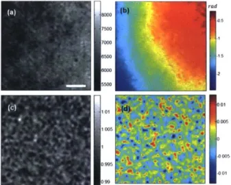
Figure 2.3 (a), (b) Amplitude and phase, respectively, of the raw interferograms in absence of any sample. (c), (d) Corresponding corrected amplitude and phase maps. Scale bar is 2.5

pm.

An alternate way of achieving higher sensitivity is recording more images and averaging the frames, which is effectively increasing the number of collected photons on each pixel while sacrificing temporal resolution. As shown in Table 2.1, amplitude noise improves with an increase in the number of the averaged frames, i.e., with a 10 times increase in the number of frames, we observe

vrih

x 10

2 (a _1.006

2 (a) Average Phase F uumm M.0 C Average Arnplitude Fluchuaton

0 200 400 600 800 1000 0 200 400 600 800 100 frames (d) Frequency Spectrum

I

A

. 1

-- IL

.

Figure 2.4 (a), (c) Variations in the average phase and amplitude over time, respectively. (b), (d) Frequency spectra of the phase and amplitude fluctuations. The vertical axes of the frequency spectra are normalized relative to the peak value.

Next, we record interferograms using a novel Adimec camera (model # Q-2A750/CXP) with a superior full well depth of about 1,600,000 electrons. We record interferograms at 600 fps for 2 seconds with an illumination wavelength of

A

Mira 900, Coherent Inc.). Our analysis of the fringe pattern shows an effective camera count of about

835,000 electrons that corresponds to a sensitivity of roughly 1.1 x 10-3. Each diffraction-limited spot

is again sampled over 7 camera pixels and each interference fringe is sampled using four pixels in this case, which is consistent with the theoretical framework. Therefore, the theoretical limit for sensitivity is expected to be about 4.1 x 10-4 that matches well with experimental results. By increasing the number of averaged frames from I to 10, phase and amplitude sensitivities improve roughly three times. However, increasing number of frames from 10 to 100 increases the phase and amplitude sensitivities

by slightly above two times, instead of the expected three-fold increase.

Table 2.1 Phase and amplitude sensitivities as a function of the number of averaged frames

Photron Adimec

phase (rad) amplitude phase (rad) amplitude

I frame 3.3 x 10-3 3.3 x 10-3 5.9 x 10-4 5.9x 10-4 10 frame 1.1 x 10-3 1.0 x 10-3 19.1 x 10-5 18.7x 10-5 100 frame 3.4x 10-4 3.3 x 10-4 8.3 x 10-5 7.2x10-5 (b) Frequency SpectuM

jou.1

L

0

The most sensitive measurement by the Adimec camera shows an optical path length stability of about 10 pm at 6 fps. Figure 2.5 shows the temporal standard deviation maps of the amplitude and phase at this speed for both cameras. As seen in Figure 2.5(a) and 2.5(b), temporal fluctuations of the amplitude and phase is relatively flat over the field of view for the case of Photron camera. However, as shown in Figure 2.5(c) and 2.5(d), there is a certain pattern present for phase and amplitude fluctuations in sensitive measurements done by the Adimec camera. This suggest we may be facing an environmental limit at a frequency around 20 Hz. Since mechanical vibration tend to happen at much higher frequencies, we speculate that this distribution could be due to a mismatch of optical path length between the reference and the sample arms in the non-common path part of the interferometer due to air-density fluctuations.

S5

~

Figure 2.5 (a), (b) standard deviation maps of the temporal fluctuations of the amplitude and phase measured by the Photron camera. (c), (d) standard deviation maps of the temporal fluctuations of the amplitude and phase measured by the Adimec camera. Scale bar is 2.5 pm

2.1 Conclusion

In this chapter, we initially lay out a theoretical framework to link the phase and amplitude sensitivity of the off-axis interferometric measurements to the intensity distribution of the fringe in the recorded interferogram at the shot noise limit. The conclusions, however, are readily extensible to the case of phase shifting interferometry where the intensity variations occur temporally for the same pixel rather than spatially over a few pixels. Following this theoretical analysis, we show experimental sensitivity values match very well with this predicted theoretical limit. This agreement means sensitivities of phase and amplitude measurements made with a conventional CMOS camera is mostly limited by photon shot noise, particularly at high imaging speeds e.g. hundreds of frames per second.

Integration of the signal through averaging of the frames can improve measurement sensitivities until we face environmental disturbances at approximately 20 Hz in our case. Therefore, when integration time is faster than approximately 50 ms, the measurement sensitivities improves by the square root of the number of the averaged frames, as expected. However, as noted earlier integration in time will compromise the temporal resolution of the measurements and does not improve sensitivity when integration time is beyond 50 ms (i.e. 20 Hz environmental noise). Using a novel camera with more than a million full electron well capacity, we show that contribution of the shot noise can be significantly reduced and sub-milliradian sensitivity can be achieved at high-speed single frame measurements. Through temporal averaging, sensitivity can be further improved, achieving an optical path stability of a few picometers. Our conclusion is that sensitivity at this order is limited by the air-density fluctuations even for near-common path interferometers. We are designing next generation interferometers that can even better reduce these residual non-common path environmental effects.

Chapter 3

Scanning Color Optical

Tomography (SCOT)

We have developed an interferometric optical microscope that provides three-dimensional refractive index map of a specimen by scanning the color of three illumination beams. Our design of the interferometer allows for simultaneous measurement of the scattered fields (both amplitude and phase) of a complex input beam. By obviating the need for mechanical scanning of the illumination beam or detection objective lens; the proposed method can increase the speed of the optical tomography by orders of magnitude.

* _{The content of this chapter is published as,}

3.1 Introduction

Digital Holographic Microscopy (DHM) provides unique opportunities to interrogate biological specimens in their most natural condition with no labeling and minimal phototoxicity. The refractive index is the source of the image contrast in DHM, which can be related to the average concentration of non-aqueous contents within the specimen, the so-called dry mass (31-33). Tomographic interrogation of living biological specimens using DHM can thereby provide the mass of cellular organelles (34) as well as three-dimensional morphology of the subcellular structures within cells and small organisms (35). There are other label-free approaches (36, 37) that rely on non-linear light-matter interactions to provide rich molecular-specific information. Compared to such nonlinear techniques, DHM can significantly reduce the damage to the specimens and minimally interferes with the cell physiology, because the scattering cross-section of the linear light-matter interaction is much higher. Therefore, DHM is highly suitable for monitoring morphological developments and metabolism of cells and small organisms over an extended period (38, 39). Recently, DHM was also used to quantify cellular differentiation, which promises an exciting opportunity for the regenerative medicine where labeling is often not a viable option (40).

A variety of DHM techniques have been demonstrated to measure both the amplitude and phase

alterations of the incident beam due to the interrogated sample (29, 41). In transmission phase measurements, the refractive index of the sample and its height are coupled; the measured phase can be due to the variation in either height or refractive index distribution within the sample. One approach to acquire the depth-resolved refractive index map is to record two-dimensional phase maps at multiple illumination angles and use a computational algorithm for the three-dimensional reconstruction. The illumination angle on a sample can be varied either by rotating the sample (42) as shown in Figure

3.1(a) or by rotating the illumination beam (35, 43, 44), as shown in Figure 3.1(b). To achieve higher

stability, common-path adaptations of the angle-scan technique were recently presented (45, 46). Tomographic cell imaging has also been demonstrated using partially-coherent light, where the focal plane of objective lens was axially scanned through the sample (47-50), see Figure 3.1(c). It is worth nothing that the speed of the data acquisition in these techniques is limited by the mechanical scanning of a mirror or the sample stage. Recently, in our center, we have demonstrated three-dimensional cell imaging using a focused line beam, as shown in Figure 3.1(d), which allows interrogation of the cells as translated on a mechanical stage (51) or continuously flowing in a microfluidic channel (52).

In this chapter, we present a unique three-dimensional cell imaging technique that completely obviates the need for scanning optical elements of a microscope. In the proposed method, the depth

information is acquired by scanning the wavelength of illumination, which was first proposed in the ultrasound regime (53). Because scanning the wavelength of a single illumination beam does not provide good depth sectioning, we split the beam into three branches, each of which is collimated and incident onto the specimen at a different angle Figure 3.1(e). Both the phase and amplitude images corresponding to the three beams are recorded in a single shot for each wavelength using our novel phase microscope. The wavelength is scanned using an acousto-optic tunable filter whose response time is only tens of microseconds, several orders of magnitude faster than mechanical scanning (54). In the following sections, we explain the theoretical framework upon which the new technique is founded, and the experimental setup allowing for the measurements required by the theory. Applying our method to polystyrene beads and live biological specimens, we demonstrate the three-dimensional imaging capability of the proposed system for a practically attainable color-scan range of 430nm

-630nm.

(a) Unicolor Coherent Ilhunination (b) Coherent Angle-Scanning

(e) Color Scanning Optical Tomography

sample rotalios

(c) Partially-Coherent Illumination (d) Focused-beam illumination +0

white ight sample

l jctive scan

Figure 3.1 Tomographic optical microscopy in various configurations for three-dimensional refractive index mapping of a

specimen: (a) Rotating-sample geometry (42). (b) Rotating-beam geometry (35, 43, 44). (c) Objective-lens-scan geometry (47-50). (d) Scanning-sample geometry (51, 52), and (e) color-scan geometry proposed in this study. The figure (e) also shows the spatial (XY,Z) coordinates used for derivation of the formula

3.2 Scanning color optical tomography (theory)

Suppose that we illuminate a sample with a collimated beam at certain wavelength and record the amplitude and phase of the scattered field from the sample. The recorded images will contain the information of the sample's structure and refractive index. Specifically, the scattered field recorded for a collimated beam of a specific color and illumination angle contains the sample information lying on the Ewald sphere in the spatial frequency space (53). The arc C in Figure 3.2(a) represents a cross-section of the Ewald sphere, where the radius of arc is the inverse of the wavelength and its angular

extent is determined by the numerical aperture of the imaging system. Thus by varying the color of illumination, we will retrieve a different portion of the object's spatial-frequency spectrum. This additional information on the sample effectively improves the three-giimensional imaging capability, as was first explained in the context of ultrasonic tomography (53). It is important to note that reconstructing the three-dimensional refractive index map of the sample from this mapping in the spatial-frequency space is an ill-posed inverse problem (55), which becomes better posed to solve as we retrieve more regions of the spatial-frequency space by performing additional measurements. One may define the axial resolution of the system as the inverse of the bandwidth or frequency support in the Kz direction. It must be noted that this axial resolution is not necessarily the same for all the transverse frequencies.

(d) (e) (t) 1

1.57

1.56

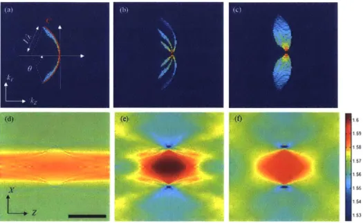
Figure 3.2 Mapping of the two-dimensional scattered fields in the spatial frequency space for different wavelengths and

illumination angles: (a) Single-beam illumination. (b) Three-beam illumination (0, +0 and -0), and (c) continuous scanning of the illumination angle from -0 to +0. For this simulation, 0 = 320 was used. Figures (d)-(f) are X-Z cross-sections of the refractive index map reconstructed from (a)-(c), respectively. The wavelength is varied from 430 to 630 nm. Imaging objective (60X, NA=1.2). Scale bar is I Opm.

Application of the wavelength-scan approach for optical microscopy has been discouraged due to the fact that one needs to scan the wavelength over an impractically broad range to achieve reasonably high depth resolution. For a more quantitative assessment of this argument, we simulated three imaging geometries using a I 0-pm polystyrene microsphere (immersed in index matching oil of

n = 1.56) as a sample. In the first simulation, we assumed that a single collimated beam was incident

and 3.2(d) show the vertical cross-sections of retrieved frequency spectrum and reconstructed tomogram, respectively. The spatial-frequency support in Figure 3.2(a) is narrow, which explains the elongated shape of bead along the z-direction in Figure 3.2(d). Increasing the wavelength range up to

830 nm did not make a visible improvement on the image. This result is consistent with previous studies

(56), which showed that wavelength scan alone does not provide the sufficient coverage in the

spatial-frequency space. To get around this limitation, we introduce two additional beams to the sample and change their illumination color at the same time. Figure 3.2(b) shows a cross-section of the retrieved frequency spectrum when three beams are introduced at the angles of 0, +0 and -0 with respect to the optical axis and their colors are changed simultaneously. The reconstructed bead for this case, shown in Figure 3.2(e), converges to the true shape of the bead. To make a comparison with the angle-scan tomography, shown in Figure 3.1(b), we further simulated the case where the sample was illuminated with a single beam at 530 nm, the average wavelength, and the angle of illumination was varied from

-0 to +0. As one may expect, the retrieved spatial-frequency spectrum in Figure 3.2(c) is now

continuous, however, the spatial-frequency coverage in the z-direction is comparable to the case of the wavelength scan using three beams. This could be also visually seen from a comparison between the extent of the frequency support in the Kz direction for Figure 3.2(b) and 3.2(c).

Interferometry-based techniques are highly suitable for measuring the complex amplitude (both amplitude and phase) of the scattered field in the visible range. To record the scattered field of the three incident beams, we built an instrument (see Figure 3.3) adapted from a Diffraction Phase Microscope (DPM)( 19). Specifically, the output of a broadband source (Fianium SC-400) is tuned to a specific wavelength through a high-resolution acousto-optic tunable filter (AOTF) operating in the range from 400 to 700 nm. The filter bandwidth linearly increases with the wavelength, but stays in the range of 2-7 nm; therefore, we may assume that the illumination used for each measurement is quasi-monochromatic. The output of the AOTF is coupled to a single-mode fiber, collimated and used as the input beam to the setup. A Ronchi grating (40 lines/mm, Edmund Optics Inc.) is placed at a plane (IPo) conjugate to the sample plane (SP) in order to generate three beams incident on the sample at different angles. Note that other than the condenser (Olympus 60 X, NA = 0.8) and the collector lens

(f3 = 200 mm) we use a 4F imaging system (fi = 30 mm,f2= 50 mm) in order to better adjust the beam

diameter and the incident angle on the sample. Using a 4F imaging system also facilitates filtering the beams diffracted by the grating so that only three beams enter the condenser lens. Three collimated beams pass through the microscope objective lens (Nikon 60 X, A = 1 .2) and tube lens

(f=

plane (IP2). There is another 4F imaging system between the grating and the CCD camera (f5 = 100

mm,f6 = 300 mm). The focal lengths of the lenses and the grating period are chosen to guarantee that

one period of the grating is imaged over approximately four camera pixels (12). As shown in Figure

3.3, there are nine diffracted orders at the Fourier plane, as opposed to three in the conventional DPM.

Three columns correspond to three angles of incidence on the sample while three rows are due to diffraction by the grating in the detection arm. We apply a low-pass filter on the strongest diffracted beam at the center to use it as a reference for the interference. The recorded interferogram provides the information of the sample carried by the three beams. Therefore, the recorded interferogram contains three interference patterns, two of which are oblique (I and III) and the third (II) is vertical. While the three patterns may not be distinguishable in the raw interferogram, one can isolate the information for each incident angle in the spatial frequency domain, i.e., by taking the Fourier transform of the interference pattern. Ipi f2 FP1 fi IN *1kP Phyukl Mask (M~) fs Collector Lens

-#

-

r-Y---[

Figure 3.3 Schematic diagram of the experimental setup: SP (Sample plane); IP (Image plane); FP (Fourier Plane); Condenser

lens (Olympus 60 X, NA = 0.8), Objective lens (Nikon 60 X, NA = 1.2). fi = 30 mm,2 = 50 mm,3 = 200 mm,f4 = 200 mm,

f5 = 100 mm, and f6 = 300 mm. Non-diffracted order is shown in red while yellow refers to the oblique illumination.

Interferograms I, II, and III are decomposition of the raw interferogram (bottom right) into its three components. The physical mask placed at FP2, creates a reference by spatially cleaning the non-diffracted order while passing the I ' order sample beams that correspond to the three incident angles

3.3 Data analysis and experimental results

We use an illumination consisting of three beams and record two-dimensional scattered fields after the specimen for different wavelengths. For a monochromatic, plane-wave illumination, the

i

Z'

-

16

scattered field after specimen can be simply related to the scattering potentialf of the specimen in the spatial frequency space. To briefly summarize the theoretical background used for data analysis, the scattering potential is defined as

f H

)=

where Ao is the wavelength in the vacuum, ko=27/lo is the wave number in the free space, n,, is the refractive index of surrounding medium, and n(r) is the complex refractive index of the sample (57). Ignoring the polarization effects of the specimen, the complex amplitude u(r) of the scattered field satisfies the following scalar wave equation,

[V2 + k 2u,(F)= f(i)u(F), k = n. ko (3.2)

where k is the wave number in the medium, and u(r) is the total field, which is recorded by the detector, and represents a sum of the incident and scattered field. A more complete theoretical framework taking the vector nature of light in tomographic techniques into account can be found here (43). When the specimen is weakly scattering, the two-dimensional Fourier transform of the scattered field recorded in various illumination conditions can be mapped onto the three-dimensional Fourier transform of the scattering potential of the object, as was first proposed by E. Wolf (57):

F(kx,ky,kzj =(ikz/ff)exp(-ikzz)U(k,k,;z),

(3.3) k=7k2 -k|-k 2

where F(kxky,kz) is the three-dimensional Fourier transform of scattering potential f(XYZ), and

U.(k,kyz) is the two-dimensional Fourier transform of the scattered field u,(x,yz) with respect to x and

y. The variables kx, ky, and kzare the spatial frequency components in the object coordinates, while kx,

ky and kz refer to the those in the laboratory frame. Therefore, one needs to map the scattered field of

the transmitted waves for each illumination condition to the right position in the three-dimensional Ewald's sphere discussed earlier,

kX =k -k m,

ki, =k,1-k m,, (3.4)

kz =k:-k

_l-m

where m. and m, are functions of the illumination, which are proportional to the location of of the object's zero frequencies in the object coordinate. In the case of off-axis interferometry these parameters can be readily calculated using the two-dimensional Fourier transform of the scattered waves, see Figure 3.4. The original formulation in Eq. (3.3) was derived using the first-order Born

approximation., A. Devaney later extended this formulation to allow for the first-order Rytov approximation as well, which resulted in better reconstruction of optically thick specimens (58). The Rytov formulation use the same equation, Eq. (3.3), after substituting the scattered field defined as:

(3.5)

p, (F) = ln [u()/uo (F)].

where uo(x,y;z) is the incident field. The Rytov approximation is valid when the following criterion is met,

n, >>[kVqj2 . (3.6)

where n8 is the refractive index change within the sample. Therefore, the Rytov approximation is valid when the phase change of propagating light is not large over the wavelength scale. This is in contrast to Born approximation where the total change in the phase itself must be small rather than the phase gradient (53).

Lky

rad

6

4

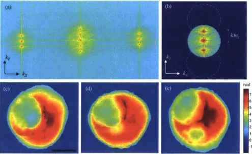
Figure 3.4 Data processing. (a) Two-dimensional Fourier transform of the raw interferogram, whose magnitude is shown in

a logarithmic scale of base 10. (b) Cropping the spatial frequencies using masks defined by the physical numerical aperture. The circles are centered at the object zero frequency location corresponding to the illumination angle. Blue dots show the center points. (c)-(e) Phase maps after unwrapping, which correspond to +0, normal, -0 beams, respectively. Scale bar is 1 Opm.

In off-axis interferometry adopting a single illumination beam, one can simply extract both the amplitude and phase of the measured field using the Hilbert Transform applied to the raw interferogram

(18, 19). In our method adopting three beams, we need to isolate the contribution of each beam prior