HAL Id: hal-02285340
https://hal.archives-ouvertes.fr/hal-02285340
Submitted on 16 Sep 2019
HAL is a multi-disciplinary open access
archive for the deposit and dissemination of
sci-entific research documents, whether they are
pub-lished or not. The documents may come from
L’archive ouverte pluridisciplinaire HAL, est
destinée au dépôt et à la diffusion de documents
scientifiques de niveau recherche, publiés ou non,
émanant des établissements d’enseignement et de
torque nano-oscillators under conservative and
dissipative driving signals
J. Hem, Liliana D. Buda-Prejbeanu, U. Ebels
To cite this version:
J. Hem, Liliana D. Buda-Prejbeanu, U. Ebels.
Power and phase dynamics of injection-locked
spin torque nano-oscillators under conservative and dissipative driving signals. Physical Review B:
Condensed Matter and Materials Physics (1998-2015), American Physical Society, 2019, 100 (5),
pp.054114. �10.1103/PhysRevB.100.054414�. �hal-02285340�
Power and phase dynamics of injection locked spin torque
nano-oscillators under conservative and dissipative driving signals
J. Hem
1, L.D. Buda-Prejbeanu
1and U. Ebels
11 Univ. Grenoble Alpes, CEA, CNRS, Grenoble INP1, IRIG-Spintec, 38000 Grenoble, France
To describe all possible injection locking configurations of spin torque nano-oscillators (STNO), previous analytical descriptions are extended by introducing the most general form of the driving
force: ℱ ∝ + . We provide the expressions of the corresponding forcing
functions ℱ for the six basic conservative and dissipative forcing torques ( ~ × and ~ × × with = , , ), and demonstrate at the example of a uniform in-plane magnetized STNO, that the general case (| | | |) as well as special cases, can occur depending on: (i) the nature of the forcing torque, (ii) the direction with respect to the equilibrium direction, (iii) the harmonic order and (iv) the operation point (dc current). These relations provide a straightforward means to analyze more complex forcing torques such as a rotating field or the superposition of damping-like and field-like spin transfer torques. Besides the phase properties we also address in detail the power properties of the injection locked state for which two new parameters are introduced: the locking power range and the power angle . They can provide important complementary information on the driving forces from experiment. The general description presented here is not limited to STNOs and is valid for any non-isochronous auto-oscillator driven by an elliptical forcing of conservative or dissipative nature.
I. INTRODUCTION
Many studies1,2,3,4,5,6,7,8,9have experimentally demonstrated the possibility to injection lock spin torque
nano-oscillators (STNOs) to a spin polarized rf current or an rf field. Injection locked STNOs can serve to overcome the problems associated with signal stability, can be efficient rf frequency dividers10 or can enhance
the efficiency of the conversion of rf power into a dc voltage signal for energy harvesting applications11,12. They
are also the building blocks for the development of mutually synchronized STNOs13,14,15,16,17,18 which has made
recently, for nanocontacts19,20 and nanopillars21,22, many progress in terms of experimental feasibility.
The injection locked STNO can be studied numerically by solving the Landau-Lifshitz-Gilbert-Slonczewski equation (LLGS). For example, locking to a spin polarized rf current was addressed23,24,25,26,27,28 to investigate
hysteresis and temperature effects of the locking range, the transient states, the phase slips or the role of the
field like torque. Analytically injection locking was treated for several symmetrical cases and vortex STNOs by linearization of LLGS to derive the locking range29,30,31,32 through the well-known Adler equation33. An
alternative analytical approach is based on the Hamiltonian formalism for spin waves34,35 which consists in the
transformation of the LLGS equation into a general non-isochronous auto-oscillator equation for a complex oscillator variable. This transformation was applied first to STNOs in the autonomous regime34,36, then
extended to the non-autonomous regime including external driving signals35. This framework can also explain
many properties of the injection locked STNO such as the locked phase1,2,3, the non-Adlerian transients7,26,37,
the general concepts of fractional synchronization3 and hysteretic behavior8.
While most of these descriptions focused on the locking to an rf spin polarized current and on the phase dynamics in the stationary locked state, less has been reported on: (i) the locking to rf fields3,5,8,30 or several
locking forces acting simultaneously24, (ii) the differences or common features of all different injection locking
configurations for conservative (rf fields) or dissipative (rf currents) driving signals, (iii) the properties of the locked oscillation power in addition to the locked phase26,38 and (iv) the dependence of the locking properties
on the free running oscillation power. All these issues should be addressed in order to significantly help defining efficient and robust injection locking schemes for various applications of signal generation or detection.
In order to answer these questions, we have extended existing analytical descriptions based on the Hamiltonian formalism in section II.A. The main modification to describe the dynamics of the complex oscillator variable is the introduction of a general forcing function ℱ ∝ + that is called elliptical, since the real and imaginary parts are unequal | | ≠ | |. This contrasts most descriptions of injection locked STNOs in literature that use circular forcings (| | = | |). We provide the stationary solutions of the injection locked phase as well as the power for a general non-isochronous auto-oscillator under elliptical forcing. Notably, the discussion of the power is important because it provides a new powerful tool to characterize experimentally the injection locking properties. In section II.B, we summarize the transformation of the LLGS equation to the general oscillator equation following Ref34,35. Then, we provide the corresponding transformations of the six basic
forcing torques, which are three conservative torques (~ × ) and three dissipative torques (~ × × ) with the direction of the spin polarization or driving field and = , , . Through this, we provide the
corresponding expressions of the forcing parameters and for the basic forcing torques in terms of the free running power and in the case of STNOs the ellipticity of the precession trajectory. Any other forcing torque can then be derived from this through a linear combination. In section III, the analytical results will be compared to numerical simulations for specific cases that are of interest for experiments and applications. We discuss the dependence of the power deviation vs detuning, the dependence of the synchronization properties as a function of dc current and also demonstrate that the derived expressions provide a straightforward means to analyze injection locking of more complex locking torques.
II. THEORITICAL ANALYSIS
A. General non-isochronous auto-oscillator under elliptical forcing
Stationary solutions. The dynamics of non-isochronous auto-oscillators is described by the oscillation power and the angular frequency ! = 0! + # where # is the non-linear frequency shift and 0! the angular frequency at zero power. Under injection locking to an external driving signal of the form $= %$ &'$( (with amplitude %$> 0 and the angular frequency $), the dynamics of the forced motion expressed in the rotating frame through the complex variable35,39* = + , / !, is given by Eq. 1.
*. = / ! − $1 * − 23 !* + 24 !* + ℱ , !* 1!
Here is the phase difference between the phase of the oscillator and that of the external generator = ' − '$ and n is the harmonic order defined by the ratio between the generator to the oscillator free running
frequency $≈ !.
The forcing function ℱ , !, given in Eq. 2, is written as a complex elliptical function, where the real forcing parameters > 0 and respectively scale the real and imaginary part that act on the power respectively phase.
The angle 8 defines the orientation of the forcing in the complex plane. The exact expressions of !, ! and 8 ! depend on p and and, as in the case of STNOs, on the ellipticity of the trajectory (details see Sec. II B). They reflect the way the external signal source couples to the oscillator trajectory3,36,35 and therefore have
to be derived for each type of oscillator and injection locking case separately.
In order to obtain the stationary solution of the injection locked state, Eq. 1 is linearized around the free running state35
;, ;! assuming that is shifted by a small amount = − ;≪ 1. With this, one obtains the
expressions given in Table I for the phase difference and the power deviation as a function of the frequency detuning = ;− $ and the locking range I . As compared to Ref35, I and the phase
difference ; at zero detuning = 0 are generalized to the case of elliptical forcings ℱ ;!, by rescaling the
normalized non-linear frequency shift parameter P with the ratio / . This leads to a new factor λ = P / . Here P is defined through P = # ;/2 35 with the power damping rate 2 . It is noted, that from the
expression I/%$ given in Table I, it may be tempting to conclude that I/%$ scales with , however since , depend themselves on n this dependence is more complicated and an example will be discussed in Sec. III.C for spin torque oscillators.
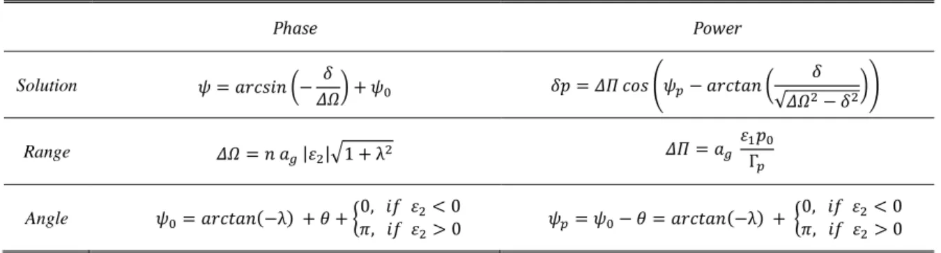
TABLE I. Summary of the solutions and the synchronization parameters (λ = P / ) for a non-isochronous oscillator under elliptical forcing.
Phase Power
Solution = %R S− IT + ; = U − %R V% S
√ I − TX
Range I = %$ | |+1 + λ = %$ Γ ;
Angle ;= %R V% −λ! + 8 + Z0, [ < 0], [ > 0 = ;− 8 = %R V% −λ! + Z0, [ < 0], [ > 0
Table I provides the expression for the power deviation , introducing two new parameters: the locking power range and the power angle. The power range gives the maximum power deviation and depends on the generator amplitude %$ as well as the ratio /2 . The latter dependence can be interpreted as
the competition between the power component of the forcing that tries to increase the power deviation and the restoring force proportional to 2 that tries to bring the oscillation back to the free running limit cycle
;.
The power angle influences strongly the shape of the power deviation within the locking range. This is demonstrated in Fig. 1 where the normalized power deviation / from Table I is plotted as a function of the normalized detuning / I for different values of . For = 0 or ]!, the power deviation describes a
half circle in the positive (negative) plane, for =]/2 (or 3]/2! it is linear and for any other value of the shape of the power deviation is a superposition of a half circle and a linear curve. Since is given by λ (see Table I) the shape of the power deviation within the locking range depends on λ and therefore contains many valuable information on the oscillator isochronicity and/or on the ratio / of the forcing parameters. The different limit cases of λ are discussed next for which the synchronization parameters simplify.
FIG.1. Normalized power deviations / as a function of the normalized detuning / I for several values of ≤ ] as
indicated on the figure. To obtain / for ≥ ] one has to use the axial symmetry & + ], ( = − , !, with a
2]-periodicity in . The special solution of = 0 leads to ! = 0 (black dashed line).
(i) Non-isochronous oscillator and/or power forcing |b| ≫ d: This case occurs when the system is very non-isochronous |P| ≫ 1 and/or when the power forcing is larger than the phase forcing parameter ≫ . As a consequence, the forcing function Eq. 2 is approximated by a “power forcing” ( ≠ 0, ≈ 0), i.e.: ℱf ≈ ℛ, ℱ!. Furthermore, takes only two possible values = ]/2 for #>0) and = 3]/2 (for #<0) and as shown in Fig. 1 the power deviation is linear and given by = / I! = / #!. This relation expresses that in
the locked regime the oscillator adapts its power to match the frequency detuning corresponding to the non-linear frequency-power dependence of the free running regime.
(ii) Isochronous oscillator and/or phase forcing |b| ≪ d: This case occurs when |P| ≪ 1 and/or | / | ≪ 1. For |P| ≪ 1, the oscillator is isochronous so that the phase difference and the power deviation will be decoupled.With = −%R V% h ≈ 0 the dependence of i describes a half circle, see Fig 1. For | / | ≪ 1, the forcing function Eq. 2 can be approximated by a “phase forcing” ( = 0, ≠ 0) that only acts on the phase difference : ℱf ≈ ℐk ℱ!. An important consequence is that in this case the variation of the power deviation is zero ( =0). Both situations |P| ≪ 1 and/or | / | ≪ 1 lead to a strong reduction of the locking range I. It is emphasized that even for large |P|, this limit case can occur when the ratio | / | ≪ 1 and an example will be given for STNOS in Sec. III.
(iii) Special cases |b|~d and |b| = |l|: For the case of |λ|~1, the full elliptical forcing function Eq. 2 has to be considered, the locking range will be enhanced moderately by ~√2 and the power deviation will be asymmetric with since ≈ ]/4 or 3]/4, (compare Fig. 1). In the case of circular forcing |λ| = |P|, the external driving signal will drive the phase and power with the same amplitude (~%$ and | | = | |). This forcing has been most often considered in the literature to discuss injection locking of STNOs35,26. Note that in
the case of large P, the circular forcing also simplifies to the power forcing discussed above. As we will see in Sec II.B, the circular forcing is not the only possible form of driving signal for STNOs. There are situations when the driving remains elliptical or reduces to a phase or power forcing. The discussion of this section on the elliptical forcing function and its special cases will therefore be relevant for experiments on spin torque oscillators as shown next.
B. Transformation of the LLGS equation using the Hamiltonian spin wave formalism
In the following injection locking of STNOs is considered where the example of a uniformly magnetized in-plane oscillator of elliptical cross-section is chosen, see Fig. 2a. The dynamics of the free layer magnetization = &kn, ko, kp(, subjected to a current spin polarized in the direction q= &k n, k o, 0(, is governed by the
. = −rst& × uvww( − rstx × & × uvww( − rst%y; z{| × & × q( + . !} V! 3!
The right hand side terms are the precession torque, the Gilbert damping torque, the spin transfer torque (STT) (called here damping-like torque DLT) and . !} is the forcing torque. rs′= r0/ 1 + x2! is the modified
gyromagnetic ratio with r; = 2.21 105 m.A-1.s-1, x the Gilbert damping constant, %
y; the DLT constant and z{| the
injected dc current density. The field-like torque (FLT) . !}~•= −rs′ €z0z*& × q( with the FLT constant €y;
is, for simplicity, neglected for the free running regime but its effect on the injection locking can be prominent and will be considered in Sec. III.E. The effective magnetic field uvww= u{|+ u{v•, defines the equilibrium direction ‚(Fig. 2a) with u{|= ƒ{| n the static applied field, u{v•= −„…†‡ the demagnetizing field, „… the saturation magnetization. †‡ is the demagnetizing tensor, its off-diagonal components are zero and its diagonal components obey the relation #pp≫ #oo> #nn. Because of this, the motion of the free layer magnetization is strongly elliptical around the x-axis with a small out-of-plane component kp. The material parameters used are summarized in Fig. 2d and some trajectories are plotted in Fig.3a.
FIG.2. (a) Schematics of the in-plane uniform oscillator with ( n, o, p) the local coordinate system and n the equilibrium
direction. (b) Frequency [;= ;/ 2]! as a function of the free running power ; (N<0), for the full range of existence of
the in-plane precession (IPP) mode defined by: 0 < ;< 0.52 or equivalently 1 < Š < 1.71 or |z|Œ| < |z{|| < 640. 10Ž•/
k². The inset shows the conversion of power to current density. It is noted that for ;> 0.52 the excitation mode changes
(d) LLGS equation Analytical model
„… (A/m) 106 ‘/’ -0.91
ƒ{| (A/m) 31831 [}“” (GHz) 6.441
x 0.02 N/(2π) (GHz) -5.030 %y; (m) -2.5x10⁻⁸ z
to an out-of plane precession42,40 that is not considered here. (c) Normalized non-linear frequency shift |P| (left scale) and
power damping rate Γ /] (right scale) vs power ;. Note that |ν|≫1 for the oscillator parameters considered here. (d) Table
of parameters used for the numerical evaluations based on equations given in the Appendix A and with dimensions of the
free layer (in nm) •n = 90, •o = 80, •p = 3.9, demagnetization factors #nn = 0.0525, #oo = 0.0594, #pp = 0.880, k n=
cos(165°), ko = sin(165°), k p = 0, linear damping Γ–/ 2]! ≈ 318 MHz, non-linear damping — ≈ −0.350. For a power of
;≈ 0.1 (corresponding to Š = 1.07 and z{| = -400x109 A/m²) one obtains: [; = 5.974 GHz, P ≈ −22 and Γ /] = 42.36 MHz.
Using the Hamiltonian formalism for spin waves described in Ref34,35, one can transform the LLGS equation Eq.
3, into the general oscillator equation Eq. 1 for the complex variable * where each torque of Eq. 3 has its equivalent in Eq. 1. The details on the precession, damping and spin transfer torque as well as the expressions of the corresponding prefactors of 0!, #, 23 !, 24 ! of Eq. 1 are given in Appendix A; It is noted that
0!, #, 23 depend on the ellipticity of the conservative orbits of which is defined through ‘/’ (with -1 ≤
‘/’ ≤ 1). The free running power is related to z{| through35 ;= Š − 1!/ Š + — !, with the supercriticality
Š = z{|/z|Œ and z|Œ = Γ–/˜ the critical current density above which stable limit cycles are stabilized. Fig. 2(b, c)
shows the evolution of the free running frequency [;= ;/ 2]!, of the amplitude relaxation frequency Γ /]
and of the non-linear coupling parameter |P| as a function of ;.
The corresponding transformation of the forcing torque . !} to the general elliptical forcing function ℱ , ! of Eq. 2 has to consider the different possible injection locking cases of STNOs. For example, a driving field ƒ$ & $V( ™, linearly polarized in a direction ™, generates a conservative forcing torque . !š=
−rt
; ƒ$ & $V( & × ™(, while injection of a current density z$ & $V(, spin polarized in a direction q=
™, generates in Eq. 3 a conservative and a dissipative forcing torque . !š = −rt; z$ & $V(& €y; × ™+ %y; × × $( due to field-like and the damping-like torque contributions. All different types of driving
signals can be obtained from a linear combination of only two basic forms of forcing torques: conservative . !}= %$ & $V( × or dissipative . !}= %$ & $V( × × ! each one for three directions in
space i = x, y, z, where ‚ is the static equilibrium direction and %$ & $V( the driving signal. The corresponding transformations are given by the basic forcing functions, written as ℱ , ! = %$›œ,• , ! where subscripts (i, n) indicate that the forcing depends on the direction and the order . For the in-plane STNO these transformations are listed in Table II, where we differentiate for clarity between conservative ›œ,•= žœ,• , ! and dissipative ›œ,•= Ÿœ,• , ! forcing functions. The detailed expressions of
the different forcing terms are quite lengthy and are provided in Appendix B. They take the form of an elliptical forcing (Eq. 2): ›œ,• , ! = ;/2!7 − 8! + − 8!9 with the power and phase forcing parameters , ‘/’ !, , ‘/’! and an additional parameter ; , ‘/’! that scales the strength %$ of the driving signal. Through ;, , the forcings ›œ,• depend on the free running power ; and the orbit ellipticity ‘/’. The detailed dependencies differ for the different orders and directions œ, but for clarity we leave out
the indices , for ;, , . From these basic forcing functions one can obtain immediately the transformation of any arbitrary forcing torque through a linear combination of the basic forcing terms ›œ,• , !, as will be illustrated in Sect. IV.E. Before discussing explicit examples, we first discuss some general properties of the forcing terms ›œ,• , !
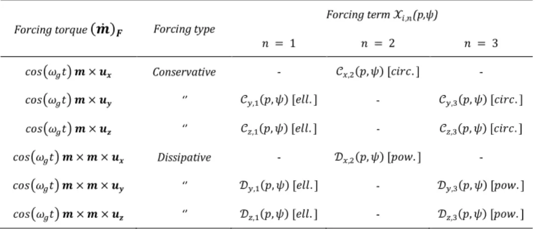
TABLE II. Summary of the transformations of the forcing torques . !š to the forcing functions ℱ , ! expressed through the forcing terms žœ,• , ! and Ÿœ,• , ! for respectively conservative and dissipative forcing and for the three directions with = , , . The forcing terms take the form of an elliptical (ell.), circular (circ.) or power (pow.) forcing, see discussion in Sect. II.A. Detailed expressions for ›œ,• , ! are given in Appendix B.
Forcing torque . !š Forcing type
Forcing term ›œ,•(p,ψ) = 1 = 2 = 3 & $V( × ‚ Conservative - žn, , ! 7 R . 9 - & $V( × ‘’ žo, , ! 7,••. 9 - žo,¡ , ! 7 R . 9 & $V( × ¢ ‘’ žp, , ! 7,••. 9 - žp,¡ , ! 7 R . 9 & $V( × × ‚ Dissipative - Ÿn, , ! 7 £. 9 - & $V( × × ‘’ Ÿo, , ! 7,••. 9 - Ÿo,¡ , ! 7 £. 9 & $V( × × ¢ ‘’ Ÿp, , ! 7,••. 9 - Ÿp,¡ , ! 7 £. 9
(i) Forcing Form: Table II shows that for STNOs all different cases of forcing can occur. More specifically, for = 1 the forcings are elliptical, for ≥ 2, the dissipative forcings Ÿœ,• , ! are power forcings ( . ,. = 0),
whereas the conservative forcings žœ,• , ! are circular forcings (i.e. | / | = 1). For many spin torque nano-oscillators one has P ≫ 1 and thus |λ| ≫ 1, so that the synchronization properties in the case of elliptical and circular forcing can be approximated by those of power forcing. As will be shown below the case of Ÿo, turns into phase forcing at specific values of the power.
(ii) Harmonic order: For both conservative and dissipative driving signals, injection locking occurs at even orders = 2, when the driving signal is along the equilibrium direction n and at odd orders = 1, 3 when it is along an orthogonal direction o or p. This confirms experiments and simulations using rf fields and currents3,4,23 .
(iii) Ellipticity ¤/¥: The exact expressions in Appendix B show that ;, , depend on the orbit ellipticity ‘/’. An important consequence is that for |‘/’| = 0 (i.e. for circular orbits) injection locking cannot occur at ≥ 2 (power and circular forcings) since here = = 0. This is consistent with descriptions for out-of-plane precessions23,38 either for a driving by field or current injection. When |‘/’| is non-zero, each case has
to be analyzed separately since not only the forcing parameters , , but also the nonlinear parameters P and Γ depend on |‘/’|, see Appendix A.
(vi) Power dependence: An important aspect of the optimization of the injection locking is to define the operational conditions that for instance provide large locking ranges. Therefore one should inspect in more detail the dependence of the locking parameters of Table I on the power p0 or equivalently on the injected dc
current density.
From Appendix B the forcing terms ›œ,• , ! for ≥ 2 are circular or power forcings that depend only on which is proportional to ;¦§ ¨ = 0,1,2 or 3). With I~ ;!P ;!, and P decreasing with ;, see Fig. 2c, the locking range I can thus either increase or decrease with ; and each injection locking case has to be analyzed separately to determine the best operation.
A more interesting situation occurs for = 1. Here the forcings žo, žp, , Ÿo, Ÿp, (see Appendix B) are elliptical functions, with more complex dependencies of , on ;. From these dependencies two critical values of power can be derived: {o for Ÿo, where = 0 and |o for žo, where = 0. As a consequence this leads to singularities in the ratio |ε /ε | and in |h| vs. ; as shown in Fig. 3(b,c) for the in-plane oscillator (with ‘/’ ≈ −0.91). For small powers ( ;< 0.1! the ratio | / | ≈ 1 and žo, , žp, , Ÿo, , Ÿp, behave all as circular forcings. Upon increasing ; the forcings žp, , Ÿp, remain almost circular while for žo, and Ÿo, the ratio | / | and |h| vary a lot, turning žo, into a power forcing at |o (|h| ≫ 1! and Ÿo, into a phase forcing at {o (|h| ≪ 1!. While
in the case of žo, one does not expect that the synchronization properties are strongly affected at |o, in the case of Ÿo, one expects at {o : (i) a strong reduction of the locking range I (absence of the non-linearity contribution), (ii) zero variation of power ( = 0 % * = 0) and (iii) in the vicinity of {o, a progressive change in the power angle . These peculiar properties are confirmed in Sec. III.B by numerical simulations. Note that for a case of strong positive ellipticity ‘/’ ≈ +1 the singularities would have led to a critical behavior in žp, , Ÿp, . These findings are an important illustration of the strong interdependence between the forcings and the orbits and that the exact forcing function has to be derived separately for each injection locking case and for the different operational points.
FIG.3. (a) 3D trajectories for the in-plane precession (IPP) mode with ‘/’ ≈ −0.91 for several free running powers ;
using the parameters of the in-plane oscillator given in Fig. 2. (b) Evolution of the ratio | / | for four different forcings at
n=1, žo, žp, Ÿo, Ÿp, over the full range of the IPP mode existence: 0 < ;< 0.52 (1 < Š < 1.71). The vertical dashed lines
correspond to the critical powers {o= 0.22 |o= 0.34 (see Appendix C). (c) Evolution of |λ| = |Pε /ε | with ;.
To conclude this part, we point out some limitations of the analytical description. (i) The transformation of the locking torques . !} for the in-plane uniform STNO provides resonant terms only for the locking order = 1, 2, 3. It does not describe injection locking for > 3 or fractional synchronization3k
$≈ s. To describe
these situations of injection locking, the analytical description needs to include additional fast oscillating terms. (ii) The analytical description is limited to small amplitudes of the driving signals, leading to linear boundaries
of the Arnold tongue defined by I/%$. This results from the approximation that the forcing functions ℱ
depend only on the free running power ; and not on the power deviation . For larger driving signals the numerical simulations43 (not shown here) reveal non-linear and asymmetrical boundaries of the Arnold tongue
as was also found in Ref8,32,44.The derived analytical expressions permit to extend the analytical description to
larger values of 43 as will be described elsewhere.
III. ANALYSIS OF SPECIFIC INJECTION LOCKING CASES
A. Macrospin solver
In the following the analytical description of Section II for the in-plane uniform oscillator will be applied to several concrete injection locking cases that are of interest for defining experiments or applications. The first case treats the injection locking for a dissipative forcing Ÿo, at n=1 applied through a spin-polarized current in the polarizer direction to illustrate the singular behavior at the critical power pdy. The second case compares
the efficiency of the injection locking by a driving field žœ,• at different orders n=1, 2, 3 and the last examples treat the superposition of two basic forcing functions. The results will be compared to macrospin simulations to validate the analytical approaches. For this the LLGS equation (Eq. 3) is numerically integrated to obtain the time evolution of the magnetization V!, using a 2nd order predictor scheme45,46 and the material parameters
of Fig. 2d. The solutions V! are then numerically transformed into V! and V!, using the transformations of Sec. II.B and are averaged over one period. The solutions are analyzed for a given set of control parameters (applied dc field Hdc and applied dc current density Jdc) upon varying the frequency detuning by varying the
frequency of the generator $. The dependencies of and on the frequency detuning are then fitted to the solutions of Table I to extract the synchronization properties ∆I, , s, , which will be compared to the corresponding results obtained from the analytical description.
B. Injection locking through the dissipative forcing ¬ ,d supplied by a spin polarized current Injection locking by an rf current density z$ & $V( at = 1, spin polarized along the polarizer direction $=
= &k ,k , 0( illustrates the forcing Ÿo, , !. The corresponding forcing torque . !š and the forcing function are given in Eq. 4:
. !š= −rst z$%y; & $V( /ko × & × (1 4%! ℱ , ! = −rst z$%y;k oŸo, , ! 4€!
with the forcing term Ÿo, , ! given in Table B4 and %$= −rs′ z$%y;ko.
Fig. 4 shows the corresponding synchronization properties ∆I, , s, as a function of the supercriticality Š =z* /zR and for a constant ratio of z$/z*. As expected from the discussion of Fig. 3, due to the singularity at the power {o where h → 1, and where the elliptical forcing turns into phase forcing, the locking range as well as the locking power are reduced by two orders of magnitude. At the same time the phase difference at zero detuning ; exhibits a jump of ], see Fig. 4c and the power angle goes to infinity, see Fig. 4d. These
variations result from a sign change of and the ] increment of 8 at the critical point.
According to the discussion on Fig. 1, the strong change of with Š is expected to lead to a strong variation of
the power deviation ! with the supercriticality Š. This is confirmed in Fig. 5(a-c). For small Š = 1.06, the elliptical forcing function ℱ can be approximated by a power forcing using ℱf = ℛ, ℱ! because for the STNO considered here P ≫ 1. This leads to close to 3]/2 (see Sect. IIA) and a linear dependence of !, as shown in Fig. 5a. Increasing the supercriticality to Š = 1.19 the power forcing starts to turn into a phase forcing and takes a value between 3]/2 and 2], explaining the transition from a linear to a tilted parabolic dependence of !, see Fig. 5(b,c). At the critical power {o≈ 0.22, corresponding to Š ≈ 1.2, compare Fig. 3b, the analytical model predicts a pure phase forcing ℱf= ℐkℱ!, leading to =0 and hence =0. However, the simulated power range in Fig. 4b and the power deviation in Fig. 5d are small but not equal to zero, the solutions are asymmetric with the detuning and the phase difference (inset of Fig. 5d) does not show the typical arcsine shape predicted from the Adler equation. From this, it is concluded that in the close vicinity of the critical power pdy, the synchronization cannot be fully described by the analytical solutions of Fig. 1
because non-resonant terms have been neglected in the transformation (see Sec. II.B) that might start to become important to correctly describe the power variation around pdy,
Except these deviations for at the critical power, there is otherwise a very good agreement between the analytical description using Ÿo, and the numerical results for all locking parameters, see Fig. 4 and the power deviation see Fig. 5 throughout the full range of super-criticalities considered here. This confirms the validity of the analytical description, in particular the occurrence of the critical power. It is an important finding relevant for experiments since the corresponding value of the supercriticality lies in the range used in common experiments.
With respect to experiments we would like to make a general comment on the power deviation . The oscillation power discussed up to now relates to the theoretical oscillation amplitude of the complex variable
d: p=|d|². This should not be confused with the experimentally measured electrical power which in the case of
STNOs can be the power spectral density measured on a spectrum analyzer1,2,3,47 or a dc rectified signal11,12
measured by a voltmeter. In magneto-resistive nanopillars the electrical power is given by the projection of the free layer magnetization on the polarizer magnetization. Thus for a given STNO configuration it is in principle possible to establish a relation between the oscillation power p=|d|² and the measured electric signals, even though this might not be straightforward for all STNO configurations. Independent of the details of this relation, an analysis of the experimentally measured power deviation as a function of detuning should reflect the dependencies of the theoretical power deviations presented in Fig. 1. In particular for the case of power
forcing (P and/or h ≫ 1) where the power deviation varies linearly, it is expected that the experimentally
measured power deviation vs. detuning is linear with a slope that reflects the relation between the free running frequency and power. Similarly, in the case of pure phase forcing, the electrical measured power deviation is
expected to be zero. This analysis provides valuable additional information on the oscillator and its
FIG.4. Injection locking using a spin polarized current polarized along for = 1. (a) locking range I, (b) power range
, (c) phase shift at zero detuning s, (d) power angle are shown as a function of Š, in the range of 1 < Š < 1.41 (0 < ;
< 0.39) with z$/z{|= -3x10⁻³. For larger driving amplitudes, the model induces an asymmetry of the Arnold tongue and is
no longer valid. All other parameters are the same as in Fig. 2. Results are compared for simulations (open dots) and
analytical calculations using the elliptical forcing (red line) ℱ ∝Ÿ ,1 Eq. 4b.
FIG.5. Power deviation versus the normalized detuning /∆Ω for different Š using parameters of Figs. 2,4. Black dots
simulations. (a) Š = 1.06, = 277°. Grey dashed line: prediction by the exact forcing ℱ using = 275° with ≈ /N. (b)
Š = 1.17, = 316°. (c) Š = 1.19, = 337°. (d) Š = 1.20 corresponding to the critical power {o≈0.22. Grey dashed line:
prediction by the exact forcing ℱ = ℐk ℱ! with ∆Π=0 and = 0. The insets in all figures show vs. the detuning .
C. Injection locking through the conservative forcings ° ,d, °‚,±, ° ,² supplied by a magnetic field The next example will compare the efficiency of the injection locking to an external field at different orders = 1, 2, 3. We consider a linearly polarized driving field ƒ$ & $V( $, see Fig. 6a, where the field direction $=
³!, ³!, 0! lies in the − plane of the layer with ³ the angle between the applied field and the x-axis. For this case, we focus only on the phase properties I and ;. For the simulation, the forcing torque is given by Eq. 5a whereas the analytical model gives three different forcings Eq. 5(b-d) depending on the order (see Table II):
. !š= −rst ƒ$ & $V( & ³! × ‚+ ³! × o( 5%!
•V = 1, ℱ , ! = −rst ƒ$ ³!žo, , ! 5€!
•V = 2, ℱ , ! = −rst ƒ$ ³!žn, , ! 5 !
•V = 3, ℱ , ! = −rst ƒ$ ³!žo,¡ , ! 5*!
The expressions of the forcing terms žo, , !, žn, , ! and žo,¡ , ! are given in Tables B1, B3), using %$=
−rst ƒ$ ³! for = 1, 3 and %$= −rst ƒ$ ³! for = 2.
To compare the efficiency, the corresponding locking ranges are normalized by the driving field amplitude and the ratio I/ƒ$ is called here coupling sensitivity. Fig. 6(b-c), shows the evolution of the coupling sensitivity I/ƒ$ and of the phase difference ; as a function of the angle ³ of the driving field. As can be seen the
coupling sensitivities I/ƒ$ are ]-periodical with ³ and the phase differences ; are 2]-periodical. This is consistent with reported experiments3 and simulations48 where the locking range for = 1, 3 is maximum
0!. When the coupling sensitivity goes to zero, the corresponding phase difference ; exhibits a jump of ] due
to the sign change of ³ and respectively ³.
Note that for the operating point (Š = 1.06) in Fig. 6,the maximum locking range for =1 (³ = 90°) is larger than for =2 (³ = 0°), which is larger than for =3 (³ = 90°): I•µn,•¶ > I•µn,•¶ > I•µn,•¶¡, see Fig. 6b. However, this is not the case for all values of Š, for instance for Š = 1.4 (not shown here) it is I•µn,•¶ > I•µn,•¶¡> I•µn,•¶ . Hence, the locking parameters strongly depend on the operational point Š (i.e. on the
power) and it is not straightforward to predict for which order n, injection locking will be more efficient. This is a further demonstration that the exact expressions of the forcing are needed to correctly describe the injection locking behavior and to compare specific configurations.
FIG.6. Injection locking using a linearly polarized driving field applied in the ( ‚, ) plane. (a) Schematic of the
configuration. ³ is the angle between the field direction ™ and the equilibrium direction ‚. Dependence on the angle ³ of
(b) the coupling sensitivity I/ƒ$ and (c) the phase difference at zero detuning ;, for injection locking at different orders
= 1, 2, 3 (blue, red, green respectively). The supercriticality is Š = 1.06 (corresponding to ;≈ 0.1 ) and all other
parameters are the same as in Fig. 2.
D. Injection locking through two simultaneous conservative forcings ° ,d and °¢,d, supplied by a magnetic field
The analytical model presented here provides a straigthforward means to address more complicated injection locking cases that are a superposition of the basic forcing torques and consequently of the basic forcing functions defined in Table II. As an example we consider the injection locking to a rotating driving field ƒ$ $ V!
at = 1, where the dynamic direction $ V! = /0, ·o & $V(, ·p & $V −'¸(1 lies in the plane ( o, p),
orthogonal to the equilibrium direction of the magnetization. Here '¹is a fixed phase delay.
The forcing torque . !š and the analytical forcing function ℱ , ! are given in Eq. 6, where the analytical description is simplified under the assumption that |h| ≫ 1 (only power forcings):
. !š= −rst ƒ$ &·o & $V( × + ·p & $V + '¹( × ¢( 6%! ℱ , ! = −rst ƒ$/·o ′ ,o & − 8o( + ·p ′,p − 8p− '¹!1 6€!
This case is more elaborated because now, two basic forcing torques & $V( × and & $V( × ¢ contribute simultaneously to the synchronization. The related basic forcing functions are ℛ, /žo, , !1 = ′,o & − 8o( and ℛ, /žp, , !1 = ′,p − 8p! with ′ ,o= ;,o ,o/2 and ′ ,p= ;,p ,p/2 (Table B3).
The phase delay '¹between the two directions and ¢induces a polarization of the driving field. In what
follows, we will focus on: (i) a linear polarized field ('¹= 0 (]), similar to Sec. III.C) and (ii) a circular polarized
field ('¹=±]/2 and ·o = ·p).
(i) Linear polarized field
The driving field is linearly polarized along the fixed direction $ = &0, ·o, ·p( = &0, ¼!, ¼!(, defined by the angle ¼, see Fig. 7a. The linear combination of the two power forcings Eq. 6b can be reduced to the form of one power forcing: ℱ ∝ ̃ & − 8f(, where ̃ and 8f depend on the parameters of the two basic forcings ·œ,
,œ
t , 8œ with = , and with the ratio ·o/·p = V% ¼!. The locking range I and the phase difference at zero
detuning ; are then given by Eq. 7:
I = ¾ ·p Ip! + &·o Io( = |·p Ip|¿1 + À·o ,o t ·p ,pt Á 7%! ;= Â Ã Ä Ã Å Æ− %R V% À t ,o/ t ,p ·p/·o Á [ ·p ,p t > 0 Æ− %R V% À t ,o/ t ,p ·p/·o Á + ] [ ·p ,p t < 0 7€!
Here Iœ = r′ ƒ
$ 1,′ |P| is the locking range when
$ = ± œ, with = , , the angle Æ is constant and defined
by Æ= & Ç #!] + 8o+ 8p+ ]/2(/2 with = +1 if '¹ = ], or −1 if '¹ = 0. Due to the assumption of |h| ≫
1 the power range is = I/ #! and = 3]/2 is a constant.
The angular variation of the coupling sensitivity I/ƒ$ and the phase difference at zero detuning ; are illustrated for the in-plane STNO in Fig. 7(b-c) for a supercriticality Š = 1.06. The analytical description (red line) agrees very well with the simulation (dots). According to Eq. 7a, the coupling sensitivity evolves ]-periodically with the angle ¼ and it is bounded between the maximum value Io/ƒ$ at ™= ± (ℱ ∝ ℛ,&žo, (, ¼=]/2 (or 3]/2)) and the minimum value Ip/ƒ$ at ™= ± ¢ (ℱ ∝ ℛ,&žp, (, ¼=0 (or ])). The difference
between Io and Ip is determined by the ratio of the power forcings t,o/ ,p
t which in the case of STNOs
depends on the ellipticity ‘/’ (see Table B3). For the in-plane STNO considered here with ‘/’ = −0.91, this leads to a forcing ratio of ′,p/ ′,o≈ 0.2. Consequently, injection locking is by a factor of ≈ 5 more efficient when the driving field is applied along as compared to ¢. For the special case of circular orbits with ‘/’ = 0, the ratio becomes t,o/ t,p = 1 and the locking range I is independent of ¼.
The angular variation of the phase difference ; in Fig. 7c (full line for ‘/’ = −0.91 ) shows an abrupt change around ™= ± ¢ but varies smoothly around ™= ± . These peculiar variations reflect the influence of the geometry of the orbit on the synchronization properties. For comparison, the dashed line in Fig. 7c shows the special case of circular orbits with ‘/’ = 0, where ; varies linearly with the angle ¼ over a 2]-range. Such a linear dependence of the phase difference can be of interest to develop a tunable phase shifter. Upon varying the field angle, the phase shift of the oscillator can be tuned linearly over a range of 2]. A similar result has been discussed in Ref48 by numerical simulations.
FIG.7. (a-c) Injection locking at = 1 to a linear polarized driving field applied in the ( , ¢) plane with '¹= 0 : (a)
Schematic with ¼ the angle between with the driving field direction ™ and ¢. Evolution as a function of ¼ of (b) the
coupling sensitivity I/ƒ$ and (c) the phase difference at zero detuning ; for the supercriticality Š = 1.06 ( ;≈ 0.1! and
other parameters as in Fig. 2. (d-f) Injection locking at = 1 to a circularly polarized driving field applied in the ( , ¢)
plane with '¹= ]/2 and ·o = ·p : (d) Schematics to indicate the rotation sense of the rotating driving field ™ with respect
to the magnetization m: plus (minus) sign means the same (opposite) rotation sense. (e) Coupling sensitivity I/ƒ$ and
(f) phase shift at zero detuning ; as a function of supercriticality Š.
(ii) Circular polarized field
We now add a constant phase delay between the y- and z- components of the driving field in Eq. 6a to generate a circularly polarized magnetic field in the plane ( o, p). Choosing ·o = ·p= · and a phase delay '¹ = ±]/2
one arrives at two configurations indicated in Fig. 7d: for '¹=+]/2 the driving field rotates in the same
direction as the dynamical component of the magnetization and for '¹=−]/2 it rotates in the opposite
expressions of Eq. 8 that show that the locking range I is now a linear superposition of the locking ranges Ip and Io, while ; is constant, as shown in Fig. 7f.
I = Ip+ Io = IoÀ1 + ′′ ,p
,oÁ 8%!
;= ] 8€!
The important result here is that upon adjusting the phase delay '¹ it is possible to enhance or reduce the
locking range: an identical rotation sense (s=+1) of the magnetization and the driving field increases the locking range whereas an opposite rotation sense (s=-1) reduces it. This is illustrated in Fig. 7e for the corresponding coupling sensitivity I/ƒ$ as a function of supercriticality. Fig. 7e furthermore shows that for s=+1 I/ƒ$ is larger than the largest of the two locking ranges which is Io, and that overall I/ƒ$ decreases with increasing supercriticality Š . Finally, there is a good agreement between the analytical model and the simulation.
This configuration is very important for practical applications, notably the mutual synchronization of STNOs. The understanding of their coupling through the generated dynamic dipolar fields will be crucial to define a robust array of mutually synchronized oscillators. For instance, the situation described in Fig. 7(d-f) would correspond to two in-plane STNOs whose time varying y- and z- components of the magnetization define a circularly polarized dipolar field in the y-z-plane. Other configurations are the out-of-plane precession mode or a vortex STNO21 that generate a circularly polarized field in the x-y-plane. Based on the results in Fig. 7e, it
is predicted that the coupling is more efficient when each oscillator sees a global dipolar field, rotating in the same direction as the magnetization. This is actually found in experiments on dipolar coupling of vortex oscillators21.
E. Injection locking through two simultaneous forcings
To finish, we generalize the method in Sec. III.C-D of combining two forcings to any sum of two functions ›É and ›Ê of Table II. For this it is necessary to define a “global phase delay” Ë written: Ë = 8É− 8Ê− '¹, where the
(i) Ì = Í/2 or 3Í/2: In this case the combination of two forcing ›É and ›Ê leads to the properties of Eq. 7a and Eq. 7b, where the locking range depends in a non-trivial manner on the individual locking ranges and the phase difference ; can be continuously tuned via the driving components ·É, ·Ê of the two involved forcings. An important example for the case of Ë = ]/2 (3]/2) is the injection locking at = 2, using a spin polarized current with a spin polarization component along the x-axis, i.e. $. n≠ 0. Considering besides the damping-like torque (DLT) also the field-damping-like torque (FLT) the total forcing torque is !. } V! ∝ z$ & $V(Î%y; × × n+ €y; × ‚Ï and the corresponding forcing function (see Table II) is ℱ ∝ %y;ℛ,&Ÿn, ( + €y;ℛ,&žn, (.
Here %y; and €y; are respectively the DLT and the FLT coefficients. With Ë = 8{n − 8|n = 3]/2 and '¹ = 0, the zero detuning phase difference ; is modified as given in Eq. 9 for the in-plane STNO. It depends on the ratio of the two torque components €y;/%y; and the ratio of the corresponding power forcings ,|n and ,{n .
;= %R V% À ,|n ,{n
€y;
%y;Á + ]/2 + &] [ %y; ,{n < 0( 9!
In the case of a strong FLT (€y;≫ %y;) this will add a phase shift of ±]/2 to ;. However, even if the FLT is small, but ,|n ≫ ,{n , there will be a non-negligible contribution to the zero detuning phase difference. A similar result has been found to explain injection locking and mutual locking of vortex oscillators7,22. It was
shown that the field like torque cannot be neglected to interpret the experimental results. Injection locking can thus provide important information on the presence and value of the field like spin transfer torque.
(ii) For Ì = Ð or Í, the injection locking properties of the combined forcing simplify to Eq. 8a and Eq. 8b. As a consequence, similar to the rotating field discussed in Fig. 7(d-f), the locking range will be enhanced or reduced depending on the rotation sense. For example, this can be useful to elaborate more complicated injection locking schemes, where at the same time, a driving current and a field synchronize the system. The model states that an optimal increase (or resp. decrease) of the locking range is possible, when the condition Ë = 0 (or resp. ]) is fulfilled. This can be obtained by choosing an adequate forcing and phase delay '¹.
In summary, in order to treat analytically all possible injection locking configurations for STNOs, we have introduced the most general form of the forcing function ℱ, which is elliptical : ℱ ∝ + with | | ≠ | |. We first provide for such elliptical forcing the stationary solutions (Sec. II.B) for the phase difference and the power deviation . They are fully described by the four locking parameters I, , ;, that depend on the forcing parameters and as well as on the non-linear oscillator parameters P and 2 (see Table I) that can be varied through the free running power ;. Here we have introduced: (i) the power range , that defines the largest power deviation within the locking range, (ii) the power angle that defines its shape (Fig. 1) and (iii) the enhancement factor h that rescales the non-linear coupling parameter P, and through this modifies previous expressions of I, ;. Since the analytical oscillation power and the experimentally measured electrical signal can be related, it is expected that one can obtain important additional information on the locking forces from experiments when analyzing the power in the injection locked state. The results for a general elliptical forcing ℱ are valid for any non-isochronous auto-oscillator. Here they are applied to the specific case of a uniformly in-plane magnetized STNO, although this can be easily transferred to other STNO configurations by appropriate choice of the coordinate system. An important output of the paper is that we provide for the six basic forcing torques (three conservative ~ × and three dissipative ~ × × ) the explicit expressions of the corresponding forcing functions ℱ ∝ + (Table II), where the forcing parameters , depend on the free running power ; (or supercriticality Š ) and the ellipticity ‘/’ of the STNO trajectory. With this, one straightforwardly obtains the dependence of the injection locking properties I, , ;, as a function of ; (or Š) and ‘/’. This allows the analysis and comparison of different injection locking configurations vs. external control parameters (dc current and via ‘/’ applied magnetic dc field) or the anisotropy (defining ‘/’ ). The full potential of the analytical description is demonstrated when superposing two external rf driving signals at the same frequency and with a fixed phase delay. For the example of a rotating rf magnetic field we show that the locking range depends on the rotation sense. Rotating rf fields occur when considering mutual synchronization of STNOS via dipolar fields. The analytical description is expected to provide a better understanding of the mutual synchronization of several STNO devices via dipolar field and/or rf currents and will help to define robust synchronization schemes, that are also relevant for rf signal detection.
ACKNOWLEDGMENTS
J. Hem acknowledges financial support from DGA. We thank C. Dieudonné for fruitful discussions.
APPENDIX A: TRANSFORMATION of LLGS The effective field of the STNO takes the following form using reduced parameters:
uÑÒÒ =ÓÔÕÀÖ4Ö×3ÖØÚØÙ••ÚÙ 4ÖØÛ•Û Á £ Vℎ Â Ä Å Ý= r;tƒ{| Þn= −r;t„…#nn Þo= r;t„…#oo Þp= r;t„…#pp •1!
The parameters of the spin wave transformation are summarized in Table A1 and the equivalent expressions in the d-variable of each torque of the LLGS equation, Eq. 3, are shown in Table A2. The parameters of the conservative and dissipative terms are defined in Table A3. More details on the transformations can be found in Refs37,43.
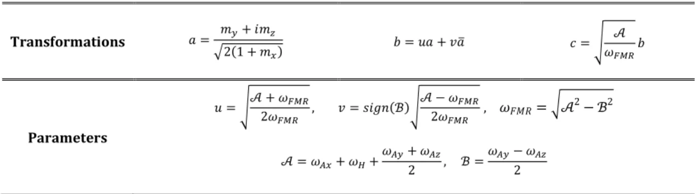
TABLE A1. Transformations of the spin wave formalism.
Transformations % = ko+ kp +2 1 + kn! € = ß% + i%à = ¿ ’ }“”€ Parameters ß = ¿’ +2 }“” }“” , i = Ç ‘!¿ ’ − }“” 2 }“” , á„â=¾’ 2− ‘2 ’ = Þn+ Ý+ Þo+2 Þp, ‘ = Þo−2 Þp
Note 1: ß, i can be expressed only through the ellipticity of the precession trajectory ‘/’.
Note 2: The non-linear factor 1/√1 − %%à coming from the first transformation is neglected in all calculations.
TABLE A2. Transformation of precession, damping and STT torques.
. = −rst& × uvww( −rstx × & × uvww( −rst%y; z{| × & × q( + . !} V!
*. = / ! − $1 * −23 !* +24 !* +ℱ , !*
! = }“”+ # 23 ! = 2– 1 + — ! Γ4 ! = ˜z{| 1 − ! Sect. II.B
TABLE A3. Coefficients of the analytical model.
Linear damping Γ$= x’
Linear spin transfer ˜ = −r;t%y;k n,
Non-linear damping
parameter — = − / ’ 1 ã3ßi&−}“” Þo+ Þp( + ß + i ! S3 Þn+32 & Þo+ Þp( + ÝTä
Non-linear frequency
shift coefficient # = − / }“”’ 1 Î3ßi ß + i !& Þp− Þo( + ßå+ iå+ 4ß i !&2 Þn+ Þo+ Þp(Ï
Power relaxation rate Γ = &ΓÇ—1+ ˜z*( 0
APPENDIX B: FORCING FUNCTIONS
TABLE B1. Circular forcings at = 2, 3 with æ ! = √1 − and for ‘/’ > 0 (If ‘/’ < 0 add +] to 8).
Forcings ›œ,• , ! =12 !,4œ ç4è!
žn, , ! ! =æ ‘/’!|‘/’| 8 = ]2
žo,¡ , ! ! = U+1 + æ ‘/’! − é Ç ‘/’!+1 − æ ‘/’!æ ‘/’! X|‘/’|2√2 + 8 =]2
žp,¡ , ! ! = U+1 + æ ‘/’! + é Ç ‘/’!+1 − æ ‘/’!æ ‘/’! X|‘/’|2√2 + 8 = ]
TABLE B2. Power forcings at = 2, 3 with æ ! = √1 − and for ‘/’ > 0 (If ‘/’ < 0 add +] to 8).
Forcings ›œ,• , ! = ! − 8!
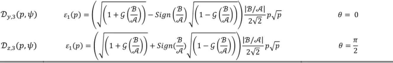
Ÿo,¡ , ! ! = ê¿À1 + æ S’TÁ − é Ç S‘ ’T ¿À1 − æ S‘ ’TÁë‘ |‘/’|2√2 + 8 = 0
Ÿp,¡ , ! ! = ê¿À1 + æ S’TÁ + é Ç ‘ ’!¿À1 − æ S‘ ’TÁë‘ |‘/’|2√2 + 8 =]2
TABLE B3. Conservative elliptical forcings at = 1 with æ ! = √1 − and with é Ç ! = 1 [ R > 0, é Ç ! = −1 [ R < 0 and S Ç ! = 0 [ R = 0. Forcings ›œ,• , ! =1 2 ; !7 ! − 8! + ! − 8!9 žo, , ! ; ! = U+1 + æ ‘/’! − é Ç ‘/’!+1 − æ ‘/’!æ ‘/’! X2+21 ! = 1 − , ! = − S1 − S2 −’T T‘ 8 = ]/2 žp, , ! ; ! = U+1 + æ ‘/’! + é Ç ‘/’!+1 − æ ‘/’!æ ‘/’! X 1 2+2 ! = 1 − , ! = − S1 − S2 +’T T‘ 8 = ]
TABLE B4. Dissipative elliptical forcings at = 1 with æ ! = √1 − , and with é Ç ! = 1 [ R > 0, é Ç ! = −1 [ R < 0 and S Ç ! = 0 [ R = 0. Forcings ›œ,• , ! =12 ; !7 ! − 8! + ! − 8!9 Ÿo, , ! ; ! = U+1 + æ ‘/’! + é Ç ‘/’!+1 − æ ‘/’!æ ‘/’! X 1 2+2 ! = ì1 − 3 S1 −’T + S1 −‘ ’T S2 −‘ ’T ì ! = −1‘ 8 = ] Ÿp, , ! ; ! = U+1 + æ ‘/’! − é Ç ‘/’!+1 − æ ‘/’!æ ‘/’! X 1 2+2 ! = ì1 − 3 S1 +’T + S1 +‘ ’T S2 +‘ ’T ì ! = −1‘ 8 =3]2
APPENDIX C: CRITICAL POWERS
The elliptical forcing Ÿo, , ! becomes a phase forcing when {o! = 0 :
{o=32 S2 − ‘/’T ê1 − ¿1 −1 49 S2 − ‘/’1 − ‘/’Të £ Vℎ ’ ∈ ã−1,‘ 15ä î1!
The elliptical forcing žo, , ! becomes a power forcing when |o! = 0:
|o =2 − ‘/’ £ Vℎ 1 ’ ∈ ã−1,‘ 12ä î2!
From symmetry, the critical power |p of žp, is given by : |p ‘/’! = |o −‘/’!, with ‘/’ ∈ 7−1/5,19 and the critical power {p of Ÿp, is given by {p ‘/’! = {o −‘/’! with ‘/’ ∈ 7−1/2,19.
REFERENCES
1 W. Rippard, M. Pufall, S. Kaka, T. Silva, S. Russek and J. Katine, Phys. Rev. Lett. 95, 067203 (2005).
2 B. Georges, J. Grollier, M. Darques, V. Cros, C. Deranlot, B. Marcilhac, G. Faini and A. Fert, Phys. Rev. Lett. 101,
017201 (2008).
3 S. Urazhdin, P. Tabor, V. Tiberkevich and A. Slavin, Phys. Rev. Lett. 105, 104101 (2010). 4 M. Quinsat et al., Appl. Phys. Lett. 98, 182503 (2011).
5 A. Hamadeh, N. Locatelli, V. V. Naletov, R. Lebrun, G. de Loubens, J. Grollier, O. Klein and V. Cros, Appl. Phys.
Lett. 104, 022408 (2014).
6 A. Dussaux et al., Appl. Phys. Lett. 98, 132506 (2011). 7 R. Lebrun et al., Phys. Rev. Lett. 115, 017201 (2015).
8 P. Tabor, V. Tiberkevich, A. Slavin and S. Urazhdin, Phys. Rev. B 82, 020407(R) (2010). 9 R. Lehndorff, D.E. Bürgler, C.M. Schneider and Z. Celinski, Appl. Phys. Lett. 97, 142503 (2010).
10 P.S. Keatley, S.R. Sani, G. Hrkac, S.M. Mohseni, P. Dürrenfeld, J. Åkerman and R.J. Hicken, Phys. Rev. B 94,
094404 (2016).
11 B. Fang et al., Nat. Commun. 7, 11259 (2016).
12 D. Tiwari, N. Sisodia, R. Sharma, P. Dürrenfeld, J. Åkerman and P.K. Muduli, Appl. Phys. Lett. 108, 082402
(2016).
13 S. Kaka, M.R. Pufall, W.H. Rippard, T.J. Silva, S.E. Russek and J.A. Katine, Nature 437, 389 (2005). 14 F.B. Mancoff, N.D. Rizzo, B.N. Engel and S. Tehrani, Nature 437, 393 (2005).
15 B. Georges, J. Grollier, V. Cros and A. Fert, Appl. Phys. Lett. 92, 232504 (2008).
16 V. Tiberkevich, A. Slavin, E. Bankowski and G. Gerhart, Appl. Phys. Lett. 95, 262505 (2009). 17 D. Li, Y. Zhou, C. Zhou and B. Hu, Phys. Rev. B 82, 140407(R) (2010).
18 J. Turtle, K. Beauvais, R. Shaffer, A. Palacios, V. In, T. Emery and P. Longhini, J. Appl. Phys. 113, 114901
(2013).
19 A. Houshang, E. Iacocca, P. Dürrenfeld, S.R. Sani, J. Åkerman and R.K. Dumas, Nat. Nanotechnol. 11, 280
(2016).
20 A.A. Awad, P. Dürrenfeld, A. Houshang, M. Dvornik, E. Iacocca, R.K. Dumas and J. Åkerman, Nat. Phys. 13,
292 (2016).
21 N. Locatelli et al., Sci. Rep. 5, 17039 (2015). 22 R. Lebrun et al., Nat. Commun. 8, 15825 (2017).
23 M. d’Aquino, C. Serpico, R. Bonin, G. Bertotti and I.D. Mayergoyz, Phys. Rev. B 82, 064415 (2010). 24 G. Finocchio, M. Carpentieri, A. Giordano and B. Azzerboni, Phys. Rev. B 86, 014438 (2012).
25 A.D. Belanovsky, N. Locatelli, P.N. Skirdkov, F. Abreu Araujo, K.A. Zvezdin, J. Grollier, V. Cros and A.K.
Zvezdin, Appl. Phys. Lett. 103, 122405 (2013).
26 Y. Zhou, V. Tiberkevich, G. Consolo, E. Iacocca, B. Azzerboni, A. Slavin and J. Åkerman, Phys. Rev. B 82,
012408 (2010).
27 Y. Zhou and J. Åkerman, Appl. Phys. Lett. 94, 112503 (2009).
28 M. d’Aquino, S. Perna, A. Quercia, V. Scalera and C. Serpico, IEEE Trans. Magn. 53, 4300905 (2017). 29 C. Serpico, R. Bonin, G. Bertotti, M. D’Aquino and I.D. Mayergoyz, IEEE Trans. Magn. 45, 3441 (2009). 30 M. Carpentieri, G. Finocchio, B. Azzerboni and L. Torres, Phys. Rev. B 82, 094434 (2010).
31 S. Perna, L. Lopez-Diaz, M. D’Aquino and C. Serpico, Sci. Rep. 6, 31630 (2016). 32 A. Quercia, M. D’Aquino, V. Scalera, S. Perna and C. Serpico, Phys. B 549, 87 (2018). 33 R. Adler, Proc. IEEE 61, 1380 (1973).
34 A. Slavin and V. Tiberkevich, IEEE Trans. Magn. 44, 1916 (2008). 35 A. Slavin and V. Tiberkevich, IEEE Trans. Magn. 45, 1875 (2009).
36 S.M. Rezende, F.M. de Aguiar and A. Azevedo, Phys. Rev. B 73, 094402 (2006). 37 M. Tortarolo et al., Sci. Rep. 8, 1728 (2018).
38 A. Hamadeh, G. de Loubens, V. V. Naletov, J. Grollier, C. Ulysse, V. Cros and O. Klein, Phys. Rev. B 85,
140408(R) (2012).
39 A. Pikovsky, M. Rosenblum and K. Jurgen, Synchronization A Universal Concept in Nonlinear Sciences
(Cambridge University Press, 2001).
40 J. Xiao, A. Zangwill and M.D. Stiles, Phys. Rev. B 72, 014446 (2005). 41 L. Lopez-Diaz et al., J. Phys. D. Appl. Phys. 45, 323001 (2012).
42 S.I. Kiselev, J.C. Sankey, I.N. Krivorotov, N.C. Emley, R.J. Schoelkopf, R.A. Buhrman and D.C. Ralph, Nature
43 J. Hem, Ph.D. thesis, Univ. Grenoble Alpes, 2018.
44 E. Jué, M.R. Pufall and W.H. Rippard, Appl. Phys. Lett. 112, 102403 (2018). 45 I. Firastrau et al., Phys. Rev. B 78, 024437 (2008).
46 J.L. García-Palacios and F.J. Lázaro, Phys. Rev. B 58, 14937 (1998). 47 E. Grimaldi et al., Phys. Rev. B 89, 104404 (2014).
![TABLE B2. Power forcings at = 2, 3 with æ ! = √1 − and for ‘/’ > 0 (If ‘/’ < 0 add + ] to 8 ).](https://thumb-eu.123doks.com/thumbv2/123doknet/13393455.405636/26.892.107.787.725.928/table-b-power-forcings-æ-gt-lt-add.webp)