1
Supplementary materials for manuscript: Resting-State EEG Topographies: Reliable and Sensitive Signatures of Unilateral Spatial NeglectSupplementary Material
In order to demonstrate that all subjects had similar spatial map per component, we first performed SVD decomposition of the EEG signal of each participant and every session. The spatial maps obtained for each participant and session were matched to the spatial maps obtained concatenating all subjects and sessions (i.e., group-level EEG-SVD maps) using Hungarian algorithm1. We computed correlation values
between the individual spatial maps and the group-level EEG-SVD maps. The correlation was high for all top-five components (mean and standard deviation across components: 0.77± 0.10 – see Supplementary Figure 1A) highlighting that all the subjects had similar spatial maps. Second, to further support the similarity across the topographies of the individual subjects, we computed a spatial regression to acquire subject-specific spatial maps. Specifically, we ran the time-concatenated SVD (i.e., concatenating all subjects and sessions) and then we regressed per subject the spatial maps of the component; i.e., we used each subject/session part of the components’ time-courses as regressors against this subject/session data to retrieve level spatial maps. We then compute the correlation between these subject-level spatial maps with the group-subject-level EEG-SVD maps obtained concatenating all subjects and sessions. The correlation was high for all top-five components (mean and standard deviation across components: 0.84 ± 0.12 – see Supplementary Figure 1B) highlighting that all the subjects had similar spatial maps and also similar to the group-level EEG-SVD topographies.
Supplementary figures
Supplementary figure 1: (A) Correlation between individual maps and group-level
EEG-SVD maps for the first five components. Error bars represent average values +/− standard error of the mean (SEM) across participants. (B) Correlation between
maps for the first five components. Error bars represent average values +/− standard error of the mean (SEM) across participants. (C) We computed EEG-SVD
decomposition concatenating separately RHD patients of group #1 and RHD patients of group #2. Bars represent correlation between EEG-SVD group-level topographical maps for RHD patients of group #1 and EEG-SVD maps for RHD patients of group #2.
Supplementary figure 2: Paper and pencil scores divided for no-neglect, mild,
and severe spatial neglect patients identified using k-means clustering algorithm. Error bars represent average values +/− standard error of the mean (SEM) for no-neglect (black bars), mild-no-neglect (grey bars), and severe no-neglect (red bars) patients. When available we report the cut-off for spatial neglect. (A) The patients were
clustered using the behavioral canonical correlation scores obtained from CCA between behavior and CVs of the EEG-SVD components. (B) The patients were
clustered using the behavioral canonical correlation scores obtained from CCA between behavior and CVs for theta and alpha bands for the P3 and P4 electrodes.
Supplementary figure 3: Chance level confusion matrix for the three-class
classifier built using the CVs of the EEG-SVD components (A) and for the three-class
classifier built using the CVs for theta and alpha bands for the P3 and P4 electrodes
3
Supplementary tables
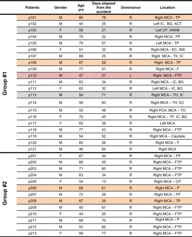
Table 1: summary of stroke patients enrolled in the study
Patients Gender Age yrs Days elapsed from the
accident Dominance Location
G
roup
#1
p101 M 66 78 R Right MCA - TP
p102 M 44 35 R Left IC, BG, ACT
p103 F 59 21 R Left CP, IHWM
p104 M 70 22 R Right MCA- FP
p105 M 79 57 R Left MCA - TP
p106 F 51 32 R Right MCA - EC, INS
p107 M 68 25 R Right MCA - Th, IC
p108 M 67 26 R Right MCA - TP
p109 M 77 91 R Right MCA - F
p110 M 47 21 L Right MCA - FTP
p111 M 63 34 R Right MCA – IC, BG
p112 F 62 32 R Left MCA – IC, BG
p113 M 54 71 R Right MCA – TH, IC
p114 M 56 60 R Right MCA – TH, EC
p115 M 53 48 R Right PCA, MCA – TO
p116 F 70 45 R Right MCA – TP, IC, BG
p117 F 65 39 R Left MCA
p118 M 77 43 R Right MCA – FTP
p119 M 54 52 R Right MCA – Caudate
p120 M 60 26 R Right MCA – F p121 M 46 84 R Right MCA
G
roup
#
2
p201 F 67 54 R Right MCA – FP p202 M 66 45 R Right MCA – FTP p203 M 71 60 R Right MCA – FTP p204 M 63 34 R Right MCA – FTP p205 F 54 13 R Right MCA – CP p206 M 66 61 R Right MCA – P p207 M 72 29 R Right MCA – FP p208 M 67 26 R Right MCA – TP p209 M 45 61 R Right MCA – FTP p210 F 44 20 R Right MCA – FTP p211 M 68 70 R Right MCA – P p212 M 53 60 R Right MCA – FTP p213 F 58 77 R Right MCA – FTPLabels in the 2nd column refer to (F) Female and (M) Male. Labels in the 5th column refer to (L) Left and (R) Right. Labels in the 6th column refer to (RHD and LHD) right and left hemisphere damage, respectively; (MCA) middle cerebral artery; F/P/T/O - Frontal/ Parietal/ Temporal/ Occipital, respectively; (STG) superior temporal gyrus; (IPL) inferior parietal lobule; (BG) basal ganglia; (IC) internal capsule; (EC) External capsule; (INS) insula; (IHWM) intra-hemishperic white matter; (TH) Thalamus. Subjects highlighted in grey were excluded from the analysis because unable to complete any of the sessions of recordings (i.e., resting-state and SNT task). The subject highlighted in pink was excluded from the analysis because
left-handed. Subjects highlighted in orange were recorded in both studies.
5
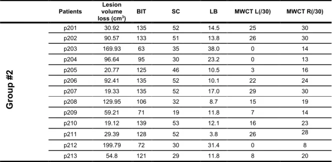
Table 2: Paper and pencil test results and volume lesion for patients of group #2Patients volume Lesion
loss (cm3) BIT SC LB MWCT L(/30) MWCT R(/30)
G
roup
#
2
p201 30.92 135 52 14.5 25 30 p202 90.57 133 51 13.8 26 30 p203 169.93 63 35 38.0 0 14 p204 96.64 95 30 23.2 0 13 p205 20.77 125 46 10.5 3 16 p206 92.41 135 52 10.1 22 24 p207 19.33 135 52 17.0 29 30 p208 129.95 106 32 8.7 15 19 p209 59.21 71 19 11.8 7 14 p210 19.12 139 53 12.1 16 23 p211 29.39 128 52 3.8 26 28 p212 199.79 72 30 31.4 0 8 p213 54.8 121 29 11.8 8 20Table 3: summary of the recordings sessions for healthy subjects and patients of group #1
Subjects Day 1 Day 2 Days between D1 and D2
Morning Afternoon Evening Morning Afternoon Evening
Healt hy su bject s c301 7 c302 5 c303 -- c304 7 c305 7 c306 7 Pat ien ts gr oup # 1 p101 7 p102 1 p104 1 p105 43 p106 11 p107 7 p108 7 p109 -- p111 7 p112 5 p114 2 p115 -- p116 2 p117 7 p118 9 p119 7 p120 1 p121 --
Green squares indicate that an entire session (i.e., resting-state and SNT task) was completed and included in the analysis.
7
Table 4: summary of the recordings sessions for patients of group #2. Days between sessions are reported as mean ± std over following sessions.Subjects Days of recordings Days between sessions
D1 D2 D3 D4 D5 D6 D7 D8 D9 D10 Pa tie nts gr oup #2 p201 4 ± 2 p202 3 ± 1 p203 2 ± 1 p204 2 ± 1 p205 3 ± 3 p206 2 ± 1 p207 1 ± 1 p208 2 ± 1 p209 2 ± 1 p210 2 ± 1 p211 2 ± 2 p212 2 ± 1 p213 1 ± 1
Green squares indicate that an entire session (i.e., resting-state and SNT task) was completed and included in the analysis.
Table 5: Percentage of outliers for healthy control (first column), LHD patients (second column), RHD patients of group #1 (third column), and RHD patients of group #2 (fourth column). Values indicate mean ± SEM over subjects. We compared the number of outliers between healthy subjects and i) LHD, ii) RHD patients of group #1, and iii) RHD patients of group #2 (one-tailed, non-paired t-test with heteroschedasticity (α=0.05)). No significant differences were found.
Healthy
subjects LHD group #1 RHD group #2 RHD %Outliers 2.08
±0.20 ±0.31 0.82 ±0.26 1.72 ±0.16 2.08
Table 6: p-values, degree of freedom of the test, and t-value of the statistical test comparing RHD patients and healthy controls for the behavioral measures for the two groups.
Hit LMRT LVRT RMRT RVRT F LI Group #1 p-value df t 0.02 13.00 2.23 0.0003 15.74 4.21 0.006 13.50 2.94 0.004 16.62 3.00 0.07 17.67 1.53 0.006 13.69 2.90 0.003 15.35 -3.15 Group #2 p-value df t 0.04 12.00 1.97 0.003 14.83 3.29 0.013 12.49 2.55 0.04 14.00 1.83 0.19 13.95 0.91 0.002 13.12 3.49 0.0002 15.54 -4.50 Table 7: test-retest correlation values for behavioral measures for patients of group #1 and group #2. (*) indicate significant correlation. For patients of group #2 the test-retest correlation was calculated between days that had all the 13 patients included in the analysis (i.e., day 1, day 3, and day 7). Values indicate mean±std over pair of days.
Hit LMRT LVRT RMRT RVRT F LI
Group #1 0.55 0.82 (*) 0.61 (*) 0.91 (*) 0.27 0.62 (*) 0.85 (*) Group #2 0.94±
0.04(*) 0.03(*) 0.95± 0.04(*) 0.90± 0.09(*) 0.80± 0.19(*) 0.67± 0.30± 0.12 0.09(*) 0.86±
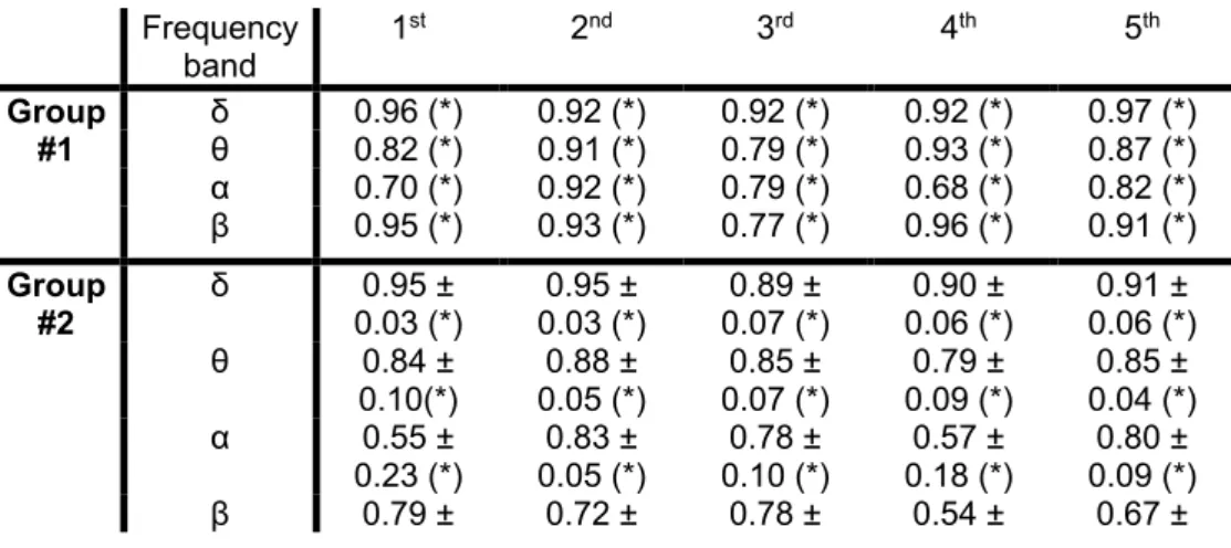
Table 8: test-retest correlation values for resting-state brain measures for patients of group #1 and group #2. (*) indicate significant correlation. For patients of group #2 the test-retest correlation was calculated between days that had all the 13 patients included in the analysis (i.e., day 1, day 3, and day 7). Values indicate mean±std over pair of days.
Frequency band 1 st 2nd 3rd 4th 5th Group #1 δ θ 0.96 (*) 0.82 (*) 0.92 (*) 0.91 (*) 0.92 (*) 0.79 (*) 0.92 (*) 0.93 (*) 0.97 (*) 0.87 (*) α 0.70 (*) 0.92 (*) 0.79 (*) 0.68 (*) 0.82 (*) β 0.95 (*) 0.93 (*) 0.77 (*) 0.96 (*) 0.91 (*) Group #2 δ 0.03 (*) 0.95 ± 0.03 (*) 0.95 ± 0.07 (*) 0.89 ± 0.06 (*) 0.90 ± 0.06 (*) 0.91 ± θ 0.84 ± 0.10(*) 0.05 (*) 0.88 ± 0.07 (*) 0.85 ± 0.09 (*) 0.79 ± 0.04 (*) 0.85 ± α 0.55 ± 0.23 (*) 0.05 (*) 0.83 ± 0.10 (*) 0.78 ± 0.18 (*) 0.57 ± 0.09 (*) 0.80 ± β 0.79 ± 0.72 ± 0.78 ± 0.54 ± 0.67 ±
9
0.01 (*) 0.13 (*) 0.06 (*) 0.11 (*) 0.19 (*)
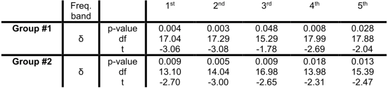
Table 9: p-values, degree of freedom of the test, and t-value of the statistical test comparing RHD patients and healthy controls for the CVs of delta band for the five EEG-SVD components and the two groups.
Freq. band 1 st 2nd 3rd 4th 5th Group #1 δ p-value df t 0.004 17.04 -3.06 0.003 17.29 -3.08 0.048 15.29 -1.78 0.008 17.99 -2.69 0.028 17.88 -2.04 Group #2 δ p-value df t 0.009 13.10 -2.70 0.005 14.04 -3.00 0.009 16.98 -2.65 0.018 13.98 -2.31 0.013 15.39 -2.47 Table 10: Number of patients (and sessions) per cluster. For the sessions we reported the mean and standard deviation over the patients of the cluster.
No-neglect
Mild-neglect Severe-neglect Group #1 11 (4±2) 9 (2±1) 8 (1.2±0.5) Group #2 10 (3±2) 12 (5±2) 5 (6±3) Reference
1 Munkres, J. Algorithms for the assignment and transportation problems. Journal of