HAL Id: hal-02408744
https://hal.archives-ouvertes.fr/hal-02408744
Submitted on 5 Dec 2020HAL is a multi-disciplinary open access archive for the deposit and dissemination of sci-entific research documents, whether they are pub-lished or not. The documents may come from teaching and research institutions in France or abroad, or from public or private research centers.
L’archive ouverte pluridisciplinaire HAL, est destinée au dépôt et à la diffusion de documents scientifiques de niveau recherche, publiés ou non, émanant des établissements d’enseignement et de recherche français ou étrangers, des laboratoires publics ou privés.
Possible patterns of marine primary productivity during
the Great Ordovician Biodiversification Event
Alexandre Pohl, David Harper, Yannick Donnadieu, Guillaume Le Hir, Elise
Nardin, Thomas Servais
To cite this version:
Alexandre Pohl, David Harper, Yannick Donnadieu, Guillaume Le Hir, Elise Nardin, et al.. Possi-ble patterns of marine primary productivity during the Great Ordovician Biodiversification Event. Lethaia, Wiley, 2018, 51 (2), pp.187-197. �10.1111/let.12247�. �hal-02408744�
Durham Research Online
Deposited in DRO:
13 October 2017
Version of attached le:
Accepted Version
Peer-review status of attached le:
Peer-reviewed
Citation for published item:
Pohl, Alexandre and Harper, David A. T. and Donnadieu, Yannick and Le Hir, Guillaume and Nardin, Elise and Servais, Thomas (2018) 'Possible patterns of marine primary productivity during the Great Ordovician Biodiversi cation Event.', Lethaia., 51 (2). pp. 187-197.
Further information on publisher's website:
https://doi.org/10.1111/let.12247
Publisher's copyright statement:
This is the accepted version of the following article: Pohl, A., Harper, D.A.T., Donnadieu, Y., Le Hir, G., Nardin, E. Servais, T. (2018) Possible patterns of marine primary productivity during the Great Ordovician Biodiversi cation Event. Lethaia, 51(2): 187-197, which has been published in nal form at https://doi.org/10.1111/let.12247. This article may be used for non-commercial purposes in accordance With Wiley Terms and Conditions for self-archiving.
Additional information:
Use policy
The full-text may be used and/or reproduced, and given to third parties in any format or medium, without prior permission or charge, for personal research or study, educational, or not-for-pro t purposes provided that:
• a full bibliographic reference is made to the original source • alinkis made to the metadata record in DRO
• the full-text is not changed in any way
The full-text must not be sold in any format or medium without the formal permission of the copyright holders. Please consult thefull DRO policyfor further details.
Possible patterns of marine primary productivity during the Great Ordovician
1
Biodiversification Event
2
3
Alexandre Pohl, David A.T. Harper, Yannick Donnadieu, Guillaume Le Hir, Elise
4Nardin & Thomas Servais
5Abstract
6
Following the appearance of numerous animal phyla during the ‘Cambrian Explosion’, the ‘Great
7
Ordovician Biodiversification Event’ (GOBE) records their rapid diversification at the lower taxonomic
8
levels, constituting the most significant rise in biodiversity in Earth’s history. Recent studies suggest
9
that the rapid rise in phytoplankton diversity observed at the Cambrian–Ordovician boundary may
10
have profoundly restructured marine trophic chains, paving the way for the subsequent flourishing
11
of plankton-feeding groups during the Ordovician. Unfortunately, the fossil record of plankton is
12
incomplete. Its smaller members represent the bulk of the modern marine biomass, but they are
13
usually not documented in Palaeozoic sediments, preventing any definitive assumption with regard
14
to an eventual correlation between biodiversity and biomass at that time. Here we use an up-to-date
15
ocean general circulation model with biogeochemical capabilities (MITgcm) to simulate the spatial
16
patterns of marine primary productivity throughout the Ordovician, and we compare the model
17
output with available palaeontological and sedimentological data.
– 160/250 words –
18
19
20
Alexandre Pohl [pohl@cerege.fr], Aix Marseille Université, CNRS, IRD, Coll France, CEREGE, Aix-en-Provence, 21
France; David A.T. Harper [david.harper@durham.ac.uk], Palaeoecosystems Group, Department of Earth
22
Sciences, Durham University, Durham DH1 3LE, UK & Department of Geology, University of Lund, SE 223 62 23
Lund, Sweden; Yannick Donnadieu [donnadieu@cerege.fr], Aix Marseille Université , CNRS, IRD, Coll France, 24
CEREGE, Aix-en-Provence, France; Guillaume Le Hir [lehir@ipgp.fr], Institut de Physique du Globe de Paris,
25
Université Paris7-Denis Diderot, 1 rue Jussieu, Paris, France; Elise Nardin [elise.nardin@get.obs-mip.fr],
26
UMR5563 Géosciences Environnement Toulouse, Observatoire Midi-Pyrénées, CNRS, Toulouse, France; 27
Thomas Servais [thomas.servais@univ-lille1.fr], Univ. Lille, CNRS, UMR 8198 - Evo-Eco-Paleo, F-59000 Lille, 28 France. 29
Introduction
30 31The ‘Great Ordovician Biodiversification Event’ (GOBE) was arguably the most important and
32
sustained increase of marine biodiversity in Earth’s history (e.g. Sepkoski 1995; Webby 2004; Harper
33
2006). During the so-called ‘Cambrian explosion’ most, if not all, animal phyla first appeared in the
34
fossil record. Subsequently, during the Ordovician Period, an ‘explosion’ of diversity at the order,
35
family, genus, and species level occurred.
36 37
The search for the triggers of this biodiversification is ongoing, but most probably there was no
38
unique cause, but the combined effects of several geological and biological processes that helped
39
generate the GOBE.
40 41
During the Ordovician Period, a unique palaeogeographical scenario existed, with the greatest
42
continental dispersal of the Palaeozoic. High sea levels that were the highest during the Palaeozoic, if
43
not of the entire Phanerozoic, allowed marine waters to cover large epicontinental areas and flooded
44
large tropical shelf areas, enabling diversification (e.g. Servais et al. 2009, 2010). The climate was
45
warm, although recent studies indicate a significant, long cooling trend throughout the Ordovician,
46
followed up by an abrupt cooling at the end of the period, triggering the Late Ordovician glacial peak
47
(Trotter et al. 2008, Nardin et al. 2011, and Harper et al. 2014).
48 49
During the Ordovician, important ecological evolutionary changes occurred, beginning with the
50
‘explosion’ of the phyto- and zooplankton, leading to the ‘Ordovician plankton revolution’ (Servais et
51
al. 2008). The onset of the GOBE is actually, at least partly for the planktonic groups, rooted in the
52
late Cambrian, when most of the planktonic organisms started to rapidly diversify (Servais et al.
53
2016). In this context, Saltzman et al. (2011) already considered that during the latest Cambrian a
54
major increase of atmospheric oxygen concentration (pO2) had already taken place. The temporal
55
correlation between the Cambrian oxygenation event and the concomitant rise in plankton diversity
56
led Saltzman et al. (2011) and Servais et al. (2016) to hypothesize that the increase of pO2 might have
57
triggered the increase of plankton diversity, which may be related to changes in macro- and
58
micronutrient abundances in increasingly oxic marine environments. The higher amount of available
59
nutrients in the oceans possibly triggered the development of pico- and phytoplankton, i.e. the basis
60
of modern marine trophic chains (Saltzman et al. 2011; Servais et al. 2016). Logically, the trophic
61
chain is then assembled with additional tiers provided by the suspension-feeding benthos (e.g.,
62
brachiopods, bryozoans and corals) and nekton, themselves prey to a range of predators, including
63
the trilobites, with orthoconic cephalopods and fishes at and near the top of the food chain.
64 65
Great advances have been made during the last decades concerning palaeogeographical
reconstructions for the Early Palaeozoic, including the Ordovician (e.g. Torsvik & Cocks 2013). These
67
more reliable global palaeogeographical reconstructions have allowed the formulation of simple
68
conceptual and more complex numerical models for ancient atmospheric and ocean circulation
69
patterns, or to hypothetically locate upwelling zones (e.g. Wilde, 1991; Christiansen & Stouge 1999;
70
Hermann et al. 2004; Pohl et al. 2014 ; Servais et al. 2014). More recently, new constraints on the
71
palaeobiogeography of marine living communities were provided by the publication of maps showing
72
much more precisely the ocean surface circulation modelled at various atmospheric CO2 levels during
73
the Early, Middle and Late Ordovician (Pohl et al. 2016b).
74 75
The aim of the present paper is to model possible patterns of biomass production in the Ordovician
76
seas, in order to attempt to understand where and how the diversification originated. We use here
77
an ocean-atmosphere general circulation model with biogeochemical capabilities (MITgcm) in order
78
to simulate the changing spatial patterns of marine primary productivity in response to the
79
palaeogeographical evolution throughout the Ordovician. We subsequently attempt to compare the
80
model output with available palaeontological and sedimentological data.
81 82
Ordovician biomass and the sedimentary record
83 84
Primary productivity in ancient oceans
85Many palaeontologists have focussed on the analyses of palaeobiodiversity during the Phanerozoic
86
(e.g., Sepkoski et al. 1981; Alroy 2010; Harper et al. 2015). Such studies lead to the understanding of
87
the major trends in biodiversification during Earth History, and to the discovery of the major
88
extinction phases, including the Big-Five mass extinctions. Specialists in macroevolution and
89
macroecology usually apply various statistical methods in order to better understand and interpret
90
the changing palaeobiodiversities (e.g. Sepkoski 1995; Bambach 2006; Alroy 2010; Stanley 2016). The
91
GOBE has also been recognized based on these studies.
92 93
Biodiversity is a measure of the number of biological organisms present at a given moment, but
94
usually provides no information about the abundance of these organisms. Little attention has been
95
paid to the evolution of the biomass in the oceans (e.g. Franck et al. 2006; Kallmeyer et al. 2012).
96
Similarly, the evolution of the abundance of nutrients available in the oceans during the history of
97
the Earth is only poorly known (e.g. Allmon & Martin 2014). In addition, biodiversity is not (at least
98
not directly) linked to the biomass produced (Irigoien et al. 2004; Finnegan & Droser 2008). As a
99
result, little information is available about biomass, or the primary productivity in ancient oceans,
including that during the GOBE.
101 102
A few authors attempted to understand the evolution of the marine biomass during geological time.
103
Martin (2003), for instance, analysed the fossil record of biodiversity in relation to nutrients,
104
productivity and habitat area, whereas Martin et al. (2008) investigated the evolution of ocean
105
stoichiometry (nutrient content) in order to understand the biodiversification of the Phanerozoic
106
marine biosphere. Concerning the Ordovician, Payne & Finnegan (2006) considered that during the
107
GOBE the increase in the complexity of the marine trophic chains and in the efficiency of marine
108
organisms in removing available food, from both the water column and the sediment, appears to
109
account for a secular increase in animal biomass. Based on Martin et al. (2008), Servais et al. (2016)
110
further considered that the increasing presence of planktonic organisms in the late Cambrian – Early
111
Ordovician must coincide with increasing nutrient supply, increased primary productivity and
112
expanded biomass production, that resulted during the initiation of the GOBE with a higher diversity
113
and increased abundance of plankton-feeding groups during the Ordovician. Nowak et al. (2015)
114
effectively observed a dramatic increase in diversity of the acritarchs, i.e. the organic-walled fraction
115
of the phytoplankton, in the late Cambrian – Early Ordovician interval. But do the higher diversities
116
of phytoplanktonic organisms also indicate an increased abundance of phytoplankton, and an
117
increased biomass?
118 119
Ocean productivity largely refers to the production of organic matter by ‘phytoplankton’ (e.g. Sigman
120
& Hain 2012). In summary, most of the single-celled phytoplankton are ‘photoautotrophs’ that use
121
nutrients and light to convert inorganic to organic carbon. They are subsequently consumed by the
122
‘heterotrophs,’ that include the ‘zooplankton’, the ‘benthos,’ and the ‘nekton.’ The most important
123
nutrients necessary for the phytoplankton are nitrogen (N), phosphorus (P), iron (Fe), and silicon (Si),
124
while sunlight is the basic energy source needed. Until recently, it was assumed that the larger parts
125
of the phytoplankton (between 5 and 100 µm in diameter) account for most phytoplankton biomass
126
and productivity. This larger phytoplankton is partly preserved in the fossil record, and corresponds
127
in the Palaeozoic to the informal group of the acritarchs. However, recent studies indicate that more
128
than half of the biomass in modern oceans is actually produced by the much smaller fraction (< 2 µm
129
in diameter), referred to the picoplankton (e.g. Buitenhuis et al. 2012). Recent estimates indicate
130
that 30 % of the modern oceanic biomass is constituted by picoheterotrophs and 25 % of
131
picophytoplankton (e.g., Buitenhuis et al. 2013; Moriarty & O’Brien 2013). This small fraction is
132
almost entirely unknown from the fossil record, the picoplankton not being observed by
133
palaeopalynologists because it falls out of the range of classical observational methods. However,
134
most recent studies indicate that it is this fraction that is the most diverse in modern oceans (e.g., De
Vargas et al. 2015).
136 137
Thus, our understanding of the fossil record of the base of the trophic chain is highly incomplete in
138
the Ordovician, as only a minor fraction of the phytoplankton is recorded under the informal
139
grouping of, for example, the acritarchs. A key approach, therefore, to tentatively understand the
140
biomass production in the Early Palaeozoic is numerical models. In the present study we apply such a
141
model for three different time intervals in the Ordovician to tentatively understand marine
142
productivity during the GOBE interval. Our analysis specifically focuses on large-scale upwelling
143
systems, which generate high rates of biomass production and leave a distinctive fingerprint in the
144
sedimentary record.
145 146
Secondary production in upwelling systems
147Modern coastal upwelling zones have been a focus of investigation for a number of years as loci of
148
bioproductivity. Here, benthic and nektonic diversity is influenced by a wide range of environmental
149
factors together with low-oxygen concentrations and biotic interactions such as competition and
150
predation. Upwelling zones promote bioproductivity through the delivery of nutrient-rich, deep
151
water onto the shelf, igniting the growth and abundance of phytoplankton. During the GOBE and
152
early stages of the establishment of the Palaeozoic Evolutionary Fauna, communities were
153
dominated by suspension feeders such as the brachiopods, bryozoans and corals and potentially
154
could benefit directly as primary consumers. There is a wealth of biodiversity data available for all
155
the major benthic and nektonic groups (e.g. Webby et al. 2004) but there are relatively few regional
156
studies related to specific geographic areas.
157 158
Recent studies of some of the key coastal upwelling zones, e.g. along the Namibian Coast (Eisenbrath
159
& Zettler 2016), associated with the Benguela Current Large Marine Ecosystem (BCLME), together
160
with those on coastal upwelling along the Peru coast (Rosenberg et al. 1983), the effects of El Nino
161
on the benthos of the Benguela, California and Humboldt upwelling ecosystems (Arntz et al. 2006)
162
and upwelling along the NW Africa coast (Thiel 1982) have established some key properties for these
163
zones. Primary and secondary production is substantial, however, it also generates low-oxygen
164
conditions commonly moving the Oxygen Minimum Zone (OMZ) into shallower-water environments.
165
Biotas are dominated by soft-bodied taxa, there is a reduced diversity and evenness and fewer
166
calcified forms (Levin 2003). In many cases assemblages are dominated by pioneer communities
167
populated by opportunistic species forming dense accumulations. Moreover, the poor oxygen
168
conditions encourage the migration of taxa into shallower water, extending too their geographic
ranges along the shelf. Organisms are abundant, generating substantial biomass but not necessarily
170
high diversities.
171 172
Methods: model description
173
Ocean, atmosphere and sea ice
174We used a coupled ocean-atmosphere-sea ice setup of the Massachusetts Institute of Technology
175
general circulation model (MITgcm). An isomorphism between ocean and atmosphere dynamics is
176
exploited to allow a single hydrodynamical core to simulate both fluids (Marshall et al. 2004). The
177
oceanic and the atmospheric components also share the same cubed-sphere grid with 32 x 32 points
178
per face (cs32), yielding a mean equatorial resolution of 2.8° x 2.8°. The cubed-sphere grid avoids
179
polar singularities resulting from the convergence of the meridians at the poles, thus ensuring that
180
the model dynamics there is treated with as much fidelity as elsewhere (Adcroft et al. 2004).
181
The oceanic component is an up-to-date, hydrostatic, implicit free-surface, partial step topography
182
ocean general circulation model (Marshall et al. 1997a, b). Twenty-eight levels are defined vertically,
183
the thickness of which gradually increases from 10 m at the surface to 1300 m at the bottom. Effects
184
of mesoscale eddies are parameterised as an advective process (Gent & McWilliams 1990) and an
185
isopycnal diffusion (Redi 1982). The nonlocal K-Profile Parameterisation (KPP) scheme of Large et al.
186
(1994) accounts for vertical mixing in the ocean’s surface boundary layer, and the interior. The
187
atmospheric physics is based on the Simplified Parameterisations, Primitive-Equation Dynamics
188
(SPEEDY) scheme (Molteni 2003). The latter comprises a four-band longwave radiation scheme, a
189
parameterisation of moist convection, diagnostic clouds, and a boundary layer scheme. A low vertical
190
resolution is used. Five levels are defined: one level represents the planetary boundary layer, three
191
layers are placed in the troposphere and the fifth layer is placed in the stratosphere. The pressure
192
coordinate p is employed. Sea ice is simulated using a thermodynamic sea-ice model based on the
193
Winton (2000) two and a half layer enthalpy-conserving scheme. Sea-ice growth occurs when the
194
ocean temperature falls below the salinity dependent freezing point.
195
Fluxes of momentum, freshwater, heat, and salt are exchanged every 20 minutes in the model (i.e.,
196
the ocean time step). The resulting coupled model can be integrated for ca. 100 years in one day of
197
dedicated computer time. Relatively similar model configurations were used in the past (Enderton &
198
Marshall 2009; Ferreira et al. 2010; 2011), including those for palaeoceanographical purposes
199
(Brunetti et al. 2015; Pohl et al. 2017).
200
Primary productivity
201The MITgcm includes a biogeochemistry model that simulates the net primary productivity (NPP) in
202
the ocean. NPP is computed based on Michaelis-Menten equations as a function of available
203
photosynthetically active radiation (PAR) and phosphate concentration (PO4),
204
205
where α = 2 × 10⁻³ mol m−3 yr−1 is the maximum community productivity, KPAR = 30 W m−2 the half
206
saturation light constant, and KPO4 = 5 × 10⁻⁴ mol m−3 the half saturation phosphate constant. In this
207
configuration, phosphate is the single limiting nutrient. It is consumed in the photic zone to fuel the
208
marine primary productivity, regenerated by remineralisation throughout the water column based
209
on the empirical law of Martin et al. (1987), redistributed within the ocean using the velocity and
210
diffusivity fields provided by the general circulation model and ultimately returned back to the ocean
211
surface in upwelling zones. Because phosphate is assumed to have an oceanic residence time much
212
longer than the oceanic turnover time scale (i.e., 10–40 kyr; Ruttenberg 1993; Wallmann 2003), its
213
global oceanic concentration is fixed in the model (Dutkiewicz et al. 2005). Iron is known as another
214
major factor in productivity (Falkowski 2012). Because it is mainly delivered to the ocean surface as
215
dust from deserts, the emissions of which are difficult to quantify today (Bryant 2013); providing the
216
model with seasonal maps of iron input in the Ordovician is challenging. Although our
217
biogeochemical model has the provision to account for cycling of iron, we prefer not to consider iron
218
fertilisation here. The PAR is computed at the ocean surface as a fraction of the incident shortwave
219
radiation provided by the atmospheric component of the MITgcm. It is then attenuated throughout
220
the water column assuming a uniform extinction coefficient. Similar configurations of this
221
biogeochemistry model have been used in the past (Friis et al. 2006; 2007), including those for the
222
Ordovician (Pohl et al., 2017).
223
Boundary and initial conditions
224We ran our model on three palaeogeographical reconstructions representative of the Early
225
Ordovician (480 Ma, Tremadocian), the Middle Ordovician (460 Ma, Darriwilian) and the early
226
Silurian (440 Ma, Aeronian). The location of the continental masses is taken from the reconstructions
227
by Torsvik & Cocks (2009). The topography and the bathymetry are reconstructed based on
228
published global reconstructions, with additional information from regional studies for Gondwana
229
(e.g. Torsvik & Cocks 2013), Laurentia (e.g. Cocks & Torsvik 2011), Baltica (e.g. Cocks & Torsvik 2005),
230
Siberia (e.g. Cocks & Torsvik 2007) and Asia (e.g. Cocks & Torsvik 2013). Because the location and
231
depth of Ordovician ocean ridges is not well constrained, they are not included in the model. We use
232
a flat-bottom ocean, the depth of which is set to present-day mean seafloor depth, i.e., –4000 m
(Pohl et al. 2014). The flat bottom is not expected to constitute a major bias. Several studies on late
234
Palaeozoic oceans suggest that it does not critically impact the large-scale patterns of simulated
235
ocean circulation (Montenegro et al. 2011; Osen et al. 2012). The resulting palaeomaps are very
236
similar to those used by Pohl et al. (Pohl et al. 2016b).
237
A gradual greening of the continents occurred throughout the Ordovician. The first, non-vascular
238
land plants are documented from the Middle Ordovician Dapingian (Rubinstein et al. 2010). There is
239
no evidence of plants on land before that date, including during the Tremadocian, i.e., the first time
240
slice used in the present study. In addition, the spatial cover of this primitive vegetation is difficult to
241
estimate for the remainder of the period (Edwards et al. 2015; Porada et al. 2016). As a consequence
242
we here follow previous studies (Nardin et al. 2011; Pohl et al. 2014) and impose a rocky desert
243
landscape on the continents (ground albedo of 0.24, which is potentially modified by snow).
244
During the Ordovician, the atmospheric partial pressure of CO2 (pCO2) was significantly higher than
245
today (e.g. Berner 2006). However, the MITgcm does not account for varying pCO2 levels. It is tuned
246
to the present-day pCO2. We therefore increased the solar forcing in the model to simulate various
247
climatic states (Ferreira et al. 2011) and subsequently compared the simulated temperatures with
248
Ordovician estimates. A solar constant of 350 W m-2 (instead of 342 W m-2 today) induces an increase
249
in tropical sea-surface temperatures (SSTs) up to 32.5 °C to 33.7 °C (depending on the time slice
250
considered). These values compare well with the SSTs reconstructed by Trotter et al. (2008) for the
251
Middle Ordovician based on ∂18O measurements (see their Fig. 3 in particular). Alternative values
252
would better fit the Early and the Late Ordovician SSTs, but we here aim at quantifying the impact of
253
the palaeogeographical changes on the spatial patterns of Ordovician primary productivity, all other
254
things kept equal. We therefore conduct our three simulations using a solar constant of 350 W m-2,
255
which are here selected to provide the best match with Middle Ordovician SST estimates. The orbital
256
configuration is defined with an obliquity of 23.45° and an eccentricity of 0°.
257
We use identical initial conditions in all simulations, including an homogeneous salinity of 35 psu
258
(practical salinity units) and a theoretical latitudinal gradient of ocean temperature characterised by
259
equatorial and polar SSTs of respectively 35 °C and 6 °C and an ocean bottom potential temperature
260
of 3 °C. These values ensure that the ocean is sea ice free at the beginning of each model run.
261
Phosphate is initialised with its present-day depth profile. For each simulation, the physical
ocean-262
atmosphere-sea ice model is first run until deep-ocean equilibrium is reached (≥ 2000 model years).
263
It is subsequently restarted with marine biogeochemistry for 550 additional years and climatic fields
264
used for analysis are averaged over the last 50 years of the simulation.
265
Results: simulated Ordovician marine productivity
267
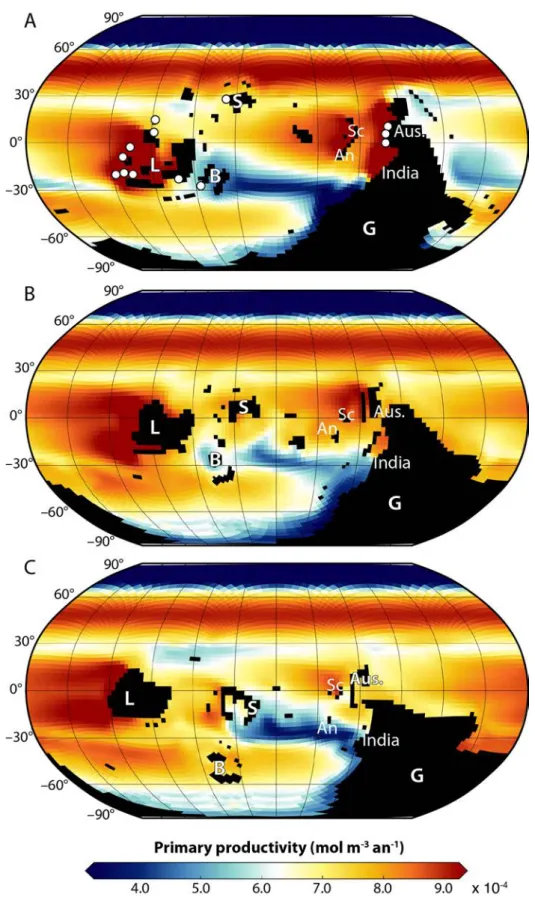
In space: wind belts and Ekman pumping
268The main patterns of simulated Ordovician surface primary productivity (Fig. 1) reflect in simple
269
terms the ocean phosphate concentration, while the PAR only imposes a hemispheric-scale decrease
270
of NPP with latitude. The phosphate concentration in surface seawaters results, in turn, from the
271
large-scale patterns of Ekman pumping. The concentration in PO4 is lower in shallow waters because
272
nutrients are consumed during photosynthesis and it increases with depth due to remineralisation of
273
sinking particles. Upwelling systems allow nutrient-rich deep waters to be transported back to the
274
surface and they are therefore associated with locally high phosphate content. On the contrary,
275
down welling areas are poor in nutrients. The spatial patterns of upwelling and down welling are
276
essentially driven by the direction of the wind blowing over the ocean surface through Ekman
277
pumping and suction. The Trade Winds induce large-scale upwelling systems on the western margin
278
of tropical landmasses, and the Westerlies cause high phosphate concentrations at the mid-latitudes
279
(40° – 60°). Between the Trade Winds and the Westerlies, the down welling of surface waters along
280
the tropics (30°) leads to low phosphate levels. A local minimum in phosphate concentration and
281
thus primary productivity occurs in the Palaeo-Tethys, between the eastern coasts of Baltica and the
282
western margin of tropical Gondwana (Fig. 1A-C). Here, the down welling of surface waters combines
283
with a strong freshwater input from the continent. The latter results from the intense orographic
284
precipitation that occurs when the moisture-laden Westerlies intercept the coastal topography of
285
Gondwana. Pohl et al. (2017) demonstrated that this strong runoff to the ocean is a robust model
286
result that it not overly model-dependent. While the polar latitudes (60° – 90°) are dynamically
287
isolated from the global ocean and thus depleted in phosphate in the Northern Hemisphere (Pohl et
288
al. 2017), deep-water convection along the coast of Gondwana (e.g. Poussart et al. 1999; Herrmann
289
et al. 2004) drives the local enrichment of surface waters in nutrients, ensuring relatively high
290
productivity levels there.
291
Although the small-scale spatial patterns of simulated NPP may be model-dependent to some extent,
292
the fact that the first-order signal results from a fundamental characteristic of Earth’s climate (the
293
zonal wind belts) suggests that these results are relatively robust (Pohl et al, 2017).
294
In time: throughout the Ordovician
295The three studied time slices share a certain number of common features (Fig. 1). The western
296
margin of Laurentia, first, is associated with high levels of simulated NPP. In both hemispheres, the
297
mid-latitudes are further characterised by zonal currents inducing Ekman pumping and the upwelling
of nutrients fuelling a strong productivity. On the contrary, low marine productivity levels typify the
299
tropics (30°), the margin of Gondwana situated over the South Pole and the Northern high-latitudes.
300
A local minimum persists throughout the period at 30° S between the western coast of Gondwana
301
and the tropical landmasses.
302
Nevertheless, major changes can be observed from 480 Ma to 440 Ma (Fig. 1). The most considerable
303
alteration of the NPP patterns between the Early and the Late Ordovician resulted from the gradual
304
drift of Gondwana to the North. Confined in the Southern Hemisphere at 480 Ma, the supercontinent
305
reached 30° N at 440 Ma. The direct consequence of this continental drift was the appearance of a
306
major upwelling system at tropical latitudes in the Late Ordovician along the coasts of Gondwana
307
(Australia and India) and South China-Annamia. The contrast between the eastern and western
308
tropical coasts of Gondwana increased at the same time, with simulated NPP significantly decreasing
309
along the eastern coast of Gondwana at 440 Ma. Elsewhere, the spatial patterns of simulated NPP
310
remained relatively stable as the tropical continental masses slowly migrated to the North. This
311
continental drift prompted Siberia to slowly shift, from the Early to the Late Ordovician, from the
312
zone of minimum NPP reported previously at 30° S to the highly productive Panthalassic circumpolar
313
current. On the contrary, Baltica underwent a migration from nutrient-rich mid-latitude waters in the
314
Southern Hemisphere at 480 Ma to the depleted water masses centred on 30° S at 440 Ma.
315
316
Discussion
317
Here we compare our modelling results with the Ordovician geological record in order to validate our
318
simulations. We also discuss some enigmatic biotic events in the light of our model runs, such as the
319
sudden and widespread bioherm development that punctuated the Late Ordovician of Baltoscandia.
320
Geological evidence for upwelling systems
321During the Ordovician two key coastal areas are typified by high levels of primary productivity in the
322
model: the west coasts of Laurentia and tropical Gondwana (Fig. 1), in particular Australia and South
323
China. These modelling results are supported by geological data. Indeed, a wide range of
324
sedimentary indicators has been confirmed for a prolonged phase of upwelling across much of
325
Laurentia during the Middle and Late Ordovician related to glaciation (Pope & Steffen 2003). A
326
careful reassessment of the ages of many of the units (Leslie & Bergström 2003) indicates that the
327
formation of cherts may be much more widespread, suggesting the possibility that this is related to
328
more general phases of upwelling across the Laurentian continent. Associated biotic indicators are
329
sparse and under-developed. Graptolites, however, were most common in upwelling zones along
continental margins. In the Vinini Formation, Roberts Mountains, Nevada, for example, changes
331
within the graptolite zooplankton have been associated with fluctuating oceanographic conditions
332
and the upwelling of anoxic waters. During high-stands graptolite faunas diversified within the OMZ
333
but the ecosystem collapsed with the substantial fall of sea level associated with the end Ordovician
334
glaciation and the retreat of the OMZ (Finney et al. 2007). Elsewhere in the Great Basin the
macro-335
shelly fauna is abundant throughout much of the Ordovician, forming locally shell beds and
336
concentrations (Finnegan & Droser 2005), with individuals increasing in size (Payne & Finnegan 2006)
337
and shell thickness (Pruss et al. 2010); the faunas are never highly diverse but they are abundant.
338
Bryozoan-rich deposits, formed by another suspension feeder, have also been associated with the
339
upwelling of nutrients in parts of Laurentia during the later Ordovician (Taylor & Sendino 2010).
340
In detail the location of the large-scale upwelling systems simulated in the model is in relatively good
341
agreement with most of the evidence of upwelling (cherts and phosphate deposits) documented by
342
Pope & Steffen (2003) (Fig. 1A). Best match is observed on the western margin of the tropical
343
landmasses, i.e., Laurentia and Gondwana. Some data points are more difficult to explain (e.g., in
344
southeastern Laurentia), and the most outstanding model-data mismatch is observed in Baltica.
345
Clearly, our simulation provides no explanation for the preservation of cherts in that precise location.
346
In order to explain the discrepancy, we emphasize that the spatial resolution of our model (ca. 300
347
km) does not allow us to capture small-scale processes. In addition, the land-sea mask interpolated
348
on the model’s grid constitutes a crude approximation of Ordovician coastlines. Finally, current
349
palaeogeographical reconstructions only provide first-order indications of Early Palaeozoic
350
bathymetry and topography and they generate large uncertainties in the position of the continental
351
masses (up to 15° in latitude) (Lees et al. 2002), which makes any straightforward model-data
352
comparison challenging.
353
To explain the appearance of these unusual carbonates with abundant chert and phosphate, Pope &
354
Steffen (2003) required the strengthening of the meridional overturning circulation and associated
355
increased nutrient supply to the ocean surface in response to glacial onset during the late Middle
356
Ordovician. Because similarly high levels of primary productivity are simulated on the western
357
margin of Laurentia during each of the three studied time slices (Fig. 1A-C), with no ice sheet over
358
the South Pole, our model suggests that such coastal upwelling may instead have been a persistent
359
characteristic of Ordovician oceans. These results are supported by the reappraisal of the age of
360
many of the deposits originally reported by Pope & Steffen (2003), a number of them being
361
potentially Early Ordovician in age (Leslie & Bergström 2003). Together this raises serious doubts
362
about the climatic implications of the phosphatic rocks proposed by Pope & Steffen (2003). Glacial
363
onset does not seem to be a necessary condition for strong upwelling to occur along the margin of
Laurentia.
365
Another possible indicator of high levels of primary productivity is the preservation of sediments
366
enriched in organic matter. Melchin et al. (2013) published a compilation of Late Ordovician – early
367
Silurian black shale occurrence. They illustrated three time slices immediately before, during and
368
right after the Hirnantian glacial peak. Using simulations similar to ours, but focusing on the Late
369
Ordovician, Pohl et al. (2017) recently demonstrated a striking correlation between the regions of
370
high (low) primary productivity simulated in their model and the preservation of organic-rich
371
(organic-poor) sediments in the geological record of the late Katian (i.e., the first time slice of
372
Melchin et al. 2013). Similar to the cherts and phosphate deposits of Pope & Steffen (2003), the black
373
shales are documented on the western margins of equatorial Laurentia and equatorial Gondwana,
374
thus matching simulated upwelling systems (Fig. 1A). More interestingly, the deposits depleted in
375
organic matter are found around Baltica and along the coast of Gondwana over the South Pole
376
(Melchin et al. 2013), precisely where the model simulates local NPP minima (Fig. 1A). This
model-377
data agreement supports the spatial patterns of NPP simulated in the present study. It also suggests
378
that the preservation of black shales in the late Katian may have been driven by the patterns of
379
primary production at the ocean surface (Pohl et al. 2017).
380
Baltoscandian reefs and mounds
381In their comprehensive review, Kröger et al. (2016) demonstrated a critical change in the mode of
382
carbonate production across the Baltic Basin during the latest Sandbian – earliest Katian (Late
383
Ordovician, ca. 453 Ma). This boundary marked the beginning of a protracted period of widespread
384
development of reefs in shallow-water areas and mud mounds in deeper epicontinental settings. The
385
authors showed that biotic factors do not explain the initiation of Late Ordovician bioherm growth.
386
They postulated climatic and eustatic drivers and further identified the northward drift of Baltica as
387
the main determining factor for the timing of the start of the Baltic reef and mound development.
388
More specifically, they suggested that ‘the entry of Baltica in a geographical zone that allowed for a
389
widespread bioherm formation was a major factor for the Sandbian radiation of reefal and
reef-390
related organisms‘. Although the most direct effect of the latitudinal shift of Baltica was probably the
391
establishment of climatic conditions more favourable to the shallow-water carbonate factory, our
392
model runs also indicate that this northward migration made Baltica enter the nutrient-depleted
393
tropical region during the Late Ordovician (Fig. 1A). Such unparalleled oligotrophic conditions may
394
have provided the appropriate environmental background for the explosion of the bioherms on
395
Baltoscandia.
396
Limitations
398
Our simulations provide an overview of possible spatial patterns of Ordovician NPP in time and space.
399
However, it does not tell us anything about the total amount of NPP. The latter is a relatively direct
400
function of nutrient availability in the ocean, which depends in turn on the intensity of continental
401
weathering. Estimating continental weathering requires major assumptions on both the lithology and
402
vegetation cover of emerged continental masses and global climate (e.g. Goddéris et al. 2014). In
403
particular, weathering may have significantly varied throughout the Ordovician as a result of changes
404
in global climate (Trotter et al. 2008), continental configuration (Nardin et al. 2011), volcanic activity
405
(Lefebvre et al. 2010), land-ice cover (Pogge von Strandmann et al. 2017) or in response to the
406
advent of the first land plants (Lenton et al. 2012; 2016; Porada et al. 2016). Such mechanisms do lie
407
beyond what we are able to resolve using our ocean-atmosphere model. As a result, we are unable
408
to predict the trend towards an increase or a decrease in NPP throughout the period.
409
410
Conclusion
411
Numerical simulations conducted with an ocean-atmosphere general circulation model with
412
biogeochemical capabilities (MITgcm) predict the position and longevity of upwelling zones in the
413
Ordovician Earth system. Upwelling zones host specific types of ecosystems, characterised by high
414
organic productivity, abundant organisms (commonly opportunist species, often soft-bodied) but not
415
necessarily high diversities. Nevertheless, high productivity levels may have provided the primary
416
resources needed by superior consumers and thus paved the way for the development of more
417
complex trophic chains featuring more diverse taxonomic assemblages. Fossil data have, to date, not
418
been aligned with these predictions although accumulations of organic matter, bone and skeletal
419
concentrations are identifiable in the fossil record and can be correlated with characteristic
420
sediments, such as cherts, that signpost upwelling zones in deep time. The present study therefore
421
targets in-depth analysis of the smaller members of the fossil record as the logical next step towards
422
the integrated understanding of the diversification patterns throughout the early Palaeozoic.
423
424
Acknowledgments
425
The findings in this study are based on climatic fields simulated by the ocean-atmosphere general
426
circulation model MITgcm. Code for the climate model MITgcm can be accessed at http://mitgcm.org.
427
Requests for the climate model output can be sent to A.P (pohl@cerege.fr). The authors thank Peter
Doyle and Alan Owen for editorial handling. We also thank Tom Challands and Axel Munnecke for
429
helpful and constructive reviews, and the guest-editors of this volume for the invitation to submit.
430
The authors acknowledge the financial support from the CNRS (INSU, action SYSTER). A.P. and Y.D.
431
thank the CEA/CCRT for providing access to the HPC resources of TGCC under the allocation
2014-432
012212 made by GENCI. A.P. thanks Maura Brunetti from the University of Geneva and David
433
Ferreira from the University of Reading, who provided expertise that greatly assisted the research.
434
This research was funded through a CEA PhD grant CFR. This is a contribution to the IGCP Project-653,
435
‘The onset of the Great Ordovician Biodiversification Event’. D.A.T.H. acknowledges financial support
436
from the Leverhulme Trust and the Wenner Gren Foundation.
437
438
439
References
440
Adcroft, A., Campin, J.M. and Hill, C. 2004: Implementation of an atmosphere-ocean general
441
circulation model on the expanded spherical cube. Monthly Weather Review 132, 2845–2863.
442
Allmon, W.D. and Martin, R.E. 2014. Seafood through time revisited: the Phanerozoic increas in
443
marine trophic resources and its macroevolutionary consequences. Paleobiology 40, 256-287.
444
Alroy, J. 2010: The shifting balance of diversity among major marine animal groups. Science 329,
445
1191–1194.
446
Arntz, W.E., Gallardo, V.A., D. Gutiérrez, D., Isla, E., Levin, L.A., Mendo, J., Neira, C., Rowe, G.T.,
447
Tarazona, J. and Wolff, M. 2006.El Niño and similar perturbation effects on the benthos of the
448
Humboldt, California, and Benguela Current upwelling ecosystems. Advances in Geosciences 6,
449
243–265.
450
Bambach, R. K., 2006: Phanerozoic Biodiversity Mass Extinctions. The Annual Review of Earth and
451
Planetary Science 34, 127-155.
452
Berner, R.A. 2006: GEOCARBSULF: A combined model for Phanerozoic atmospheric O2 and CO2.
453
Geochimica et Cosmochimica Acta 70, 5653–5664.
454
Brunetti, M., Vérard, C. and Baumgartner, P.O. 2015: Modeling the Middle Jurassic ocean circulation.
455
Journal of Palaeogeography 4, 371–383.
456
Bryant, R.G. 2013: Recent advances in our understanding of dust source emission processes. Progress
457
in Physical Geography 37, 397–421.
458
Buitenhuis, E.T., Li, W.K.W., Lomas, M.W., Karl, D.M., Landry, M.R, Jacquet, S., 2012: Picoheterotroph
459
(Bacteria and Archaea) biomass distribution in the global ocean. Earth System Science Data 4,
460
101-106.
461
Buitenhuis, E.T., Vogt, M., Moriarty, R., Bednarsek, N., Doney, S.C., Leblanc, K., Le Quérér, C., Luo,
Y.-462
W., O’Brien, C., O’Brien, T., Peloquin, J., Schiebel, R., Swan, C., 2013: MAREDAT: towards a world
463
atlas of MARine Ecosystem DATa. Earth System Science Data 5, 227-239.
464
Christiansen, J.L. & Stouge, S., 1999: Oceanic circulation as an element in palaeogeographical
465
reconstructions: the Arenig (early Ordovician) as an example. Terra Nova 11, 73–78
466
Cocks, L.R.M. and Torsvik, T.H. 2005: Baltica from the late Precambrian to mid-Palaeozoic times: The
467
gain and loss of a terrane's identity. Earth-Science Reviews 72, 39–66.
468
Cocks, L.R.M. and Torsvik, T.H. 2007: Siberia, the wandering northern terrane, and its changing
469
geography through the Palaeozoic. Earth-Science Reviews 82, 29–74.
470
Cocks, L.R.M. and Torsvik, T.H. 2011: The Palaeozoic geography of Laurentia and western Laurussia: A
stable craton with mobile margins. Earth-Science Reviews 106, 1–51.
472
Cocks, L.R.M. and Torsvik, T.H. 2013: The dynamic evolution of the Palaeozoic geography of eastern
473
Asia. Earth-Science Reviews 117, 40–79.
474
de Vargas, C., Audic, S., Henry, N., Decelle, J., Mahe, F., Logares, R., Lara, E., Berney, C., Le Bescot, N.,
475
Probert, I., Carmichael, M., Poulain, J., Romac, S., Colin, S., Aury, J.M., Bittner, L., Chaffron, S.,
476
Dunthorn, M., Engelen, S., Flegontova, O., Guidi, L., Horak, A., Jaillon, O., Lima-Mendez, G., Luke,
477
J., Malviya, S., Morard, R., Mulot, M., Scalco, E., Siano, R., Vincent, F., Zingone, A., Dimier, C.,
478
Picheral, M., Searson, S., Kandels-Lewis, S., Tara Oceans Coordinators, Acinas, S.G., Bork, P.,
479
Bowler, C., Gorsky, G., Grimsley, N., Hingamp, P., Iudicone, D., Not, F., Ogata, H., Pesant, S., Raes,
480
J., Sieracki, M.E., Speich, S., Stemmann, L., Sunagawa, S., Weissenbach, J., Wincker, P., Karsenti,
481
E., Boss, E., Follows, M., Karp-Boss, L., Krzic, U., Reynaud, E.G., Sardet, C., Sullivan, M.B. and
482
Velayoudon, D. 2015: Eukaryotic plankton diversity in the sunlit ocean. Science 348, 1261605–
483
1261605.
484
Dutkiewicz, S., Follows, M.J. and Parekh, P. 2005: Interactions of the iron and phosphorus cycles: A
485
three-dimensional model study. Global Biogeochemical Cycles 19, GB1021.
486
Edwards, D., Cherns, L. and Raven, J.A. 2015: Could land-based early photosynthesizing ecosystems
487
have bioengineered the planet in mid-Palaeozoic times? Palaeontology 58, 803–837.
488
Eisenbarth, S. and Zettler, M.L. 2016. Diversity of the benthic macrofauna off northern Namibia from
489
the shelf to the deep sea. Journal of Marine Systems 155, 1–10.
490
Enderton, D. and Marshall, J. 2009: Explorations of atmosphere–ocean–ice climates on an
491
aquaplanet and their meridional energy transports. Journal of the Atmospheric Sciences 66,
492
1593–1611.
493
Falkowski, P. 2012: Ocean science: the power of plankton. Nature 483, S17–S20.
494
Ferreira, D., Marshall, J. and Campin, J.-M. 2010: Localization of deep water formation: role of
495
atmospheric moisture transport and geometrical constraints on ocean circulation. Journal of
496
Climate 23, 1456–1476.
497
Ferreira, D., Marshall, J. and Rose, B. 2011: Climate determinism revisited: multiple equilibria in a
498
complex climate model. Journal of Climate 24, 992–1012.
499
Finnegan, S. and Droser, M.L. 2005. Relative and absolute abundance of trilobites and
500
rhynchonelliform brachiopods across the Lower/Middle Ordovician Boundary, Eastern Basin and
501
Range. Paleobiology 31, 480-502.
502
Finnegan, S. and Droser, M.L. 2008: Body size, energetics, and the Ordovician restructuring of marine
503
ecosystems. Paleobiology 34, 342–359.
504
Finney, S.C., Berry, W.B.N. and Cooper, J.D. 2007. The influence of denitrifying seawater on graptolite
505
extinction and diversification during the Hirnantian (latest Ordovician) mass extinction event.
506
Lethaia 40, 281-291.
507
Franck, S., Bounama, C. and Bloh, Von, W. 2006: Causes and timing of future biosphere extinctions.
508
Biogeosciences 3, 85–92.
509
Friis, K., Najjar, R.G., Follows, M.J. and Dutkiewicz, S. 2006: Possible overestimation of shallow-depth
510
calcium carbonate dissolution in the ocean. Global Biogeochemical Cycles 20, GB4019.
511
Friis, K., Najjar, R.G., Follows, M.J., Dutkiewicz, S., Körtzinger, A. and Johnson, M. 2007: Dissolution of
512
calcium carbonate: observations and model results in the subpolar North Atlantic.
513
Biogeosciences 4, 205–213.
514
Gent, P.R. and McWilliams, J.C. 1990: Isopycnal mixing in ocean circulation models. Journal of
515
Physical Oceanography 20, 150–155.
516
Goddéris, Y., Donnadieu, Y., Le Hir, G., Lefebvre, V. and Nardin, E. 2014: The role of palaeogeography
517
in the Phanerozoic history of atmospheric CO2 and climate. Earth-Science Reviews 128, 122–138.
518
Harper, D.A.T. 2006: The Ordovician biodiversification: Setting an agenda for marine life.
519
Palaeogeography, Palaeoclimatology, Palaeoecology 232, 148-166.
520
Harper, D.A.T., Hammarlund. E.U. and Rasmussen, C.M.Ø. 2014. End Ordovician extinctions: A
521
coincidence of causes. Gondwanan Research 25, 1294–1307.
522
Harper, D.A.T., Zhan, R.-B. and Jin, J. 2015: The Great Ordovician Biodiversification Event: Reviewing
two decades of research on diversity's big bang illustrated by mainly brachiopod data.
524
Palaeoworld 24, 75–85.
525
Herrmann, A.D., Haupt, B.J., Patzkowsky, M.E., Seidov, D. and Slingerland, R.L. 2004: Response of
526
Late Ordovician paleoceanography to changes in sea level, continental drift, and atmospheric
527
pCO2: potential causes for long-term cooling and glaciation. Palaeogeography,
528
palaeoclimatology, palaeoecology 210, 385–401.
529
Irigoien, X., Huisman, J. and Harris, R.P. 2004: Global biodiversity patterns of marine phytoplankton
530
and zooplankton. Nature 429, 863–867.
531
Kallmeyer, J., Pockalny, R., Adhikari, R.R., Smith, D.C. and D'Hondt, S. 2012: Global distribution of
532
microbial abundance and biomass in subseafloor sediment. 109, 16213–16216.
533
Kröger, B., Hints, L. and Lehnert, O. 2016: Ordovician reef and mound evolution: the Baltoscandian
534
picture. Geological Magazine, 1–24.
535
Large, W.G., McWilliams, J.C. and Doney, S.C. 1994: Oceanic vertical mixing: a review and a model
536
with a nonlocal boundary layer parameterization. Reviews of Geophysics 32, 363–403.
537
Lees, D.C., Fortey, R.A. and Cocks, L.R.M. 2002: Quantifying paleogeography using biogeography: a
538
test case for the Ordovician and Silurian of Avalonia based on brachiopods and trilobites.
539
Paleobiology 28, 343–363.
540
Lefebvre, V., Servais, T., François, L. and Averbuch, O. 2010: Did a Katian large igneous province
541
trigger the Late Ordovician glaciation? A hypothesis tested with a carbon cycle model.
542
Palaeogeography, palaeoclimatology, palaeoecology 296, 310–319.
543
Lenton, T.M., Crouch, M., Johnson, M., Pires, N. and Dolan, L. 2012: First plants cooled the
544
Ordovician. Nature Geoscience 5, 86–89.
545
Lenton, T.M., Dahl, T.W., Daines, S.J., Mills, B.J.W., Ozaki, K., Saltzman, M.R. and Porada, P. 2016:
546
Earliest land plants created modern levels of atmospheric oxygen. Proceedings of the National
547
Academy of Sciences of the United States of America, 201604787.
548
Leslie, S.A. and Bergström, S.M. 2003. Widespread, prolonged late Middle to Late Ordovician
549
upwelling in North America: A proxy record of glaciation?: Comment and Reply. Geology 31,
e28-550
e29.
551
Levin, L.A. 2003. Oxygen minimum zone benthos: adaptation and community response to hypoxia.
552
Oceanography and Marine Biology: an Annual Review 41, 1–45.
553
Marshall, J., Adcroft, A., Campin, J.M., Hill, C. and White, A. 2004: Atmosphere-ocean modeling
554
exploiting fluid isomorphisms. Monthly Weather Review 132, 2882–2894.
555
Marshall, J., Adcroft, A., Hill, C., Perelman, L. and Heisey, C. 1997a: A finite-volume, incompressible
556
Navier Stokes model for studies of the ocean on parallel computers. Journal of Geophysical
557
Research 102, 5753–5766.
558
Marshall, J., Hill, C., Perelman, L. and Adcroft, A. 1997b: Hydrostatic, quasi-hydrostatic, and
559
nonhydrostatic ocean modeling. Journal of Geophysical Research 102, 5733–5752.
560
Martin, J.H., Knauer, G.A., Karl, D.M. and Broenkow, W.W. 1987: VERTEX: carbon cycling in the
561
northeast Pacific. Deep Sea Research 34, 267–285.
562
Martin, R.E., 2003: The fossil record of biodiversity: nutrients, productivity, habitat area and
563
differential preservation. Lethaia 36, 179-193.
564
Martin, R.E., Quigg, A., Podkovyrov, V., 2008: Marine biodiversification in response to evolving
565
phytoplankton stoichiometry. Palaeogeography, Palaeoclimatology, Palaeoecology 258, 277-291
566
Melchin, M.J., Mitchell, C.E., Holmden, C., & Štorch, P., 2013. Environmental changes in the Late
567
Ordovician-early Silurian: Review and new insights from black shales and nitrogen isotopes.
568
Geological Society of America Bulletin, 125(11-12), 1635–1670.
569
Molteni, F. 2003: Atmospheric simulations using a GCM with simplified physical parametrizations. I:
570
Model climatology and variability in multi-decadal experiments. Climate Dynamics 20, 175–191.
571
Montenegro, A., Spence, P., Meissner, K.J., Eby, M., Melchin, M.J. and Johnston, S.T. 2011: Climate
572
simulations of the Permian-Triassic boundary: Ocean acidification and the extinction event.
573
Paleoceanography 26, PA3207.
574
Moriarty, R., O’Brien, T.D., 2013: Distribution of mesozooplankton biomass in the global ocean. Earth
System Science Data 5, 45-55.
576
Nardin, E., Goddéris, Y., Donnadieu, Y., Le Hir, G., Blakey, R.C., Pucéat, E. and Aretz, M. 2011:
577
Modeling the early Paleozoic long-term climatic trend. Geological Society of America Bulletin
578
123, 1181–1192.
579
Nowak, H., Servais, T., Monnet, C., Molyneux, S.G., Vandenbroucke, T.R.A., 2015. Phytoplankton
580
dynamics from the Cambrian Explosion to the onset of the Great Ordovician Biodiversification
581
Event: a review of Cambrian acritarch diversity. Earth-Science Reviews 151, 117–131.
582
Osen, A.K., Winguth, A.M.E., Winguth, C. and Scotese, C.R. 2012: Sensitivity of Late Permian climate
583
to bathymetric features and implications for the mass extinction. Global and Planetary Change,
584
171–179.
585
Payne, J.L. and Finnegan, S. 2006: Controls on marine animal biomass through geological time.
586
Geobiology 4, 1-10.
587
Pogge von Strandmann, P.A.E., Desrochers, A., Murphy, M.J., Finlay, A.J., Selby, D. and Lenton, T.M.
588
2017: Global climate stabilisation by chemical weathering during the Hirnantian glaciation.
589
Geochemical Perspectives Letters, 230–237.
590
Pohl, A., Donnadieu, Y., Le Hir, G., Buoncristiani, J.F. and Vennin, E. 2014: Effect of the Ordovician
591
paleogeography on the (in)stability of the climate. Climate of the Past 10, 2053–2066.
592
Pohl, A., Donnadieu, Y., Le Hir, G., & Ferreira, D. 2017. The climatic significance of Late
Ordovician-593
early Silurian black shales. Paleoceanography, 32(4), 397–423.
594
Pohl, A., Donnadieu, Y., Le Hir, G., Ladant, J.B., Dumas, C., Alvarez-Solas, J. and Vandenbroucke, T.R.A.
595
2016a: Glacial onset predated Late Ordovician climate cooling. Paleoceanography 31, 800–821.
596
Pohl, A., Nardin, E., Vandenbroucke, T. and Donnadieu, Y. 2016b: High dependence of Ordovician
597
ocean surface circulation on atmospheric CO2 levels. Palaeogeography, palaeoclimatology,
598
palaeoecology 458, 39–51.
599
Pope, M.C. and Steffen, J.B. 2003: Widespread, prolonged late Middle to Late Ordovician upwelling in
600
North America: A proxy record of glaciation? Geology 31, 63–66.
601
Porada, P., Lenton, T.M., Pohl, A., Weber, B., Mander, L., Donnadieu, Y., Beer, C., Pöschl, U. and
602
Kleidon, A. 2016: High potential for weathering and climate effects of non-vascular vegetation in
603
the Late Ordovician. Nature communications 7, 12113.
604
Poussart, P.F., Weaver, A.J. and Barnes, C.R. 1999: Late Ordovician glaciation under high atmospheric
605
CO2: A coupled model analysis. Paleoceanography 14, 542–558.
606
Pruss, S.B., Finnegan, S., Fischer, W.W. and Knoll, A.H. 2010. Carbonates in skeleton-poor seas: new
607
insights from Cambrian and Ordovician strata of Laurentia. Palaios 25, 73-84.
608
Redi, M.H. 1982: Oceanic isopycnal mixing by coordinate rotation. Journal of Physical Oceanography
609
12, 1154–1158.
610
Rosenberg, R., Arntz, W. E., Chuman de Flores, E., Flores, L. A., Carbajal, G., Finger, G. & Tarazona, J.
611
1983. Benthos biomass and oxygen deficiency in the upwelling system off Peru. Journal of
612
Marine Research 41, 263–279.
613
Rubinstein, C.V., Gerrienne, P., la Puente, de, G.S., Astini, R.A. and Steemans, P. 2010: Early Middle
614
Ordovician evidence for land plants in Argentina (eastern Gondwana). New Phytologist 188,
615
365–369.
616
Ruttenberg, K.C. 1993: Reassessment of the oceanic residence time of phosphorus. Chemical Geology
617
107, 405–409.
618
Saltzman, M.R., Young, S.A. and Kump, L.R. 2011: Pulse of atmospheric oxygen during the late
619
Cambrian.
620
Sepkoski, J.J., Jr. 1995. The Ordovician Radiations: Diversification and extinction shown by global
621
genus level taxonomic data; pp. 393–396 in J. D. Cooper, M. L. Droser, and S. C. Finney (eds.),
622
Ordovician Odyssey: Short Papers, 7th International Symposium on the Ordovician System. Book
623
77, Pacific Section Society for Sedimentary Geology (SEPM), Fullerton, California.
624
Sepkoski, J.J., Bambach, R.K., Raup, D.M. and Valentine, J.W. 1981: Phanerozoic marine diversity and
625
the fossil record. Nature 293, 435–437.
626
Servais, T., Lehnert, O., Li, J., Mullins, G.L., Munnecke, A., Nützel, A., Vecoli, M. 2008: The Ordovician
Biodiversification: revolution in the oceanic trophic chain. Lethaia 41, 99–109.
628
Servais, T., Harper, D. A. T., Li, J., Munnecke, A., Owen, A. W., Sheehan, P. M. 2009: Understanding
629
the Great Ordovician Biodiversification Event (GOBE): Influences of paleogeography,
630
paleoclimate, or paleoecology? GSA Today 19 (4/5).
631
Servais, T., Owen, A.W., Harper, D.A.T., Kröger, B., Munnecke, A. 2010: The Great Ordovician
632
Biodiversification Event (GOBE): the palaeoecological dimension. Palaeogeography,
633
Palaeoclimatology, Palaeoecology 294, 99-119.
634
Servais, T., Danelian, T., Harper, D.A.T., Munnecke, A. 2014: Possible oceanic circulation patterns,
635
surface water currents and upwelling zones in the Early Palaeozoic. GFF 136, 229-233.
636
Servais, T., Perrier, V., Danelian, T., Klug, C., Martin, R., Munnecke, A., Nowak, H., Nützel, A.,
637
Vandenbroucke, T. R. A., Williams, M. Rasmussen, C. M. Ø. 2016: The onset of the ‘Ordovician
638
Plankton Revolution’ in the late Cambrian. Palaeogeography, Palaeoclimatology, Palaeoecology
639
458, 12-28.
640
Sigman, D.M. and Hain, M.P. 2012: The Biological Productivity of the Ocean. Nature Education 3,
1-641
16.
642
Stanley, S.M., 2016. Estimates of the magnitudes of major marine mass extinctions in earth history.
643
Proceedings National Academy of Sciences 113, 6325-6334.
644
Taylor, P.D. and Sendino, C. 2010. Latitudinal distribution of bryozoan-rich sediments in the
645
Ordovician. Bulletin of Geosciences 85, 565–572.
646
Thiel, H. 1982. Zoobenthos of the CINECA area and other upwelling regions. Rapp. P.-v. Réun. Cons.
647
Int. Explor. Mer. 180, 323-334.
648
Torsvik, T.H. and Cocks, L.R.M. 2009: BugPlates: linking biogeography and palaeogeography,
649
software manual. geodynamics.no. Downloaded from http://www.geodynamics.no on 30 July
650
2014.
651
Torsvik, T.H. and Cocks, L.R.M. 2013: Gondwana from top to base in space and time. Gondwana
652
Research 24, 999–1030.
653
Trotter, J.A., Williams, I.S., Barnes, C.R., Lécuyer, C. and Nicoll, R.S. 2008: Did cooling oceans trigger
654
Ordovician biodiversification? Evidence from conodont thermometry. Science 321, 550–554.
655
Wallmann, K. 2003: Feedbacks between oceanic redox states and marine productivity: A model
656
perspective focused on benthic phosphorus cycling. Global Biogeochemical Cycles 17, 1084.
657
Webby, B.D. 2004. Introduction. In: Webby, B.D., Paris, F., Droser, M.L., Percival I.G. (Eds.), The Great
658
Ordovician Biodiversification Event. Columbia University Press, New York, pp. 1-37.
659
Webby, B.D., Paris, F., Droser, M.L. and Percival I.G. (Eds.), The Great Ordovician Biodiversification
660
Event. Columbia University Press, New York
661
Wilde, P. 1991: Oceanography in the Ordovician. In Barnes, C. R., Williams, S. H. (eds.), Advances in
662
Ordovician Geology, Vol. 90, 283–298. Geological Survey of Canada.
663
Winton, M. 2000: A reformulated three-layer sea ice model. Journal of Atmospheric and Oceanic
664
Technology 17, 525–531.
665 666