Analytic progress in open string field theory

(1)

Analytic progress in open string field theory

MASSACHUSETTS INSTITUTE

by OF TECHNOLOGY

Michael Stefan Kiermaier

AUG 0 4 2009

Submitted to the Department of Physics

LIBRARIES

in partial fulfillment of the requirements for the degree of

Doctor of Philosophy

at the

MASSACHUSETTS INSTITUTE OF TECHNOLOGY

June 2009

@

Massachusetts Institute of Technology 2009. All rights reserved.

Author ...

...

Department of Physics

May 20, 2009

Certified by ...

Barton Zwiebach

Professor of Physics

Thesis Supervisor

Accepted by ...

Thomas J. Greytak

Lester Wolfe Professor of Physics, Associat eDepartment Head for Education

(2)

(3)

Analytic progress in open string field theory

by

Michael Stefan Kiermaier Submitted to the Department of Physics on May 20, 2009, in partial fulfillment of the

requirements for the degree of Doctor of Philosophy

Abstract

Open string field theory provides an action functional for open string fields, and it is thus a mani-festly off-shell formulation of open string theory. The solutions to the equation of motion of open string field theory are expected to describe consistent classical open string backgrounds. In this thesis, I present a number of analytic results in bosonic open string field theory. Firstly, I present analytic solutions to the equation of motion that describe an exactly marginal deformation of the chosen open string background. A prominent example in this class is the rolling-tachyon solution, which describes the decay of an unstable D-brane. Furthermore, I demonstrate that the Riemann surface geometry of string perturbation theory can be radically simplified using propagators of Schnabl gauge instead of Siegel gauge. In principle, this simplification allows the analytic compu-tation of arbitrary off-shell one-loop open string amplitudes. Finally, I show that this simplicity of Schnabl gauge one-loop Riemann surfaces can be combined with the knowledge of analytic so-lutions to construct an analytically computable string field theory boundary state. For all known solutions, this boundary state precisely coincides with the BCFT boundary state of the open string background that the solution is expected to describe. This construction thus confirms the physical interpretation of known analytic solutions and thus provides a nice consistency check on open string field theory.

Thesis Supervisor: Barton Zwiebach Title: Professor of Physics

(4)

(5)

Acknowledgments

I would like to thank Barton Zwiebach and Dan Freedman for their patient advising, exceptional support, and countless stimulating discussions during my time at MIT. Their advice over the past years will be invaluable for my future in academia and beyond. I thank Barton for his patience during my initial steps into research, and Dan for his patience during the fifty-mile bike ride!

I thank Yuji Okawa for taking the risk of collaborating with me at an early stage when my knowledge and research experience was still very limited. I thank Henriette Elvang for her patient and pedagogic explanations that tremendously helped me to to get started on a completely different field of research. Working with Yuji and Henriette was both an honor and a pleasure, and I am looking forward to our future work!

I also thank Stephen Naculich, Leonardo Rastelli, and Ashoke Sen for very enjoyable first collaborations, and I hope there will be many more to come!

I want to thank Gita for her invaluable support over the past years, for her help to get through sometimes stressful and difficult stages of my graduate career. You found the right balance between encouragement and distraction from physics!

I want to thank Mark for being a true friend here in Cambridge, for discussions on physics, life, and beyond. I am looking forward to crashing NYC parties with you in the future! I also want to thank Murad, Martin, Frank, Frodo, and Peter for making the trip across the Atlantic to visit Cambridge. In a new environment, there is nothing more valuable than the visit of an old friend!

I also want to thank my parents for their support and council with all the decisions that I made over the last years, and for all the wonderful trips back home that allowed me to "recharge" for future challenges!

Finally, I want to thank "Mom" Holly Kroncke for a wonderful exchange year in the US that was a formative experience and, among many other things, sparked my interest in MIT. A decade later, that dream actually became true!

(6)

(7)

Chapter 1 Introduction

The action principle has traditionally been a central concept for the formulation of theories in physics. In many theories, from mechanics to the standard model of elementary particle physics, an action function (or functional) is used to determine the equations of motion for the degrees of freedom in the theory and to calculate quantum effects through the path integral formalism. Applying the action principle to string fields, however, turns out to pose enormous challenges. While the action of bosonic open string field theory [1] and the action of bosonic closed string field theory [2] have been known for many years, the equations of motion derived from them are notoriously hard to solve. In 2005, nearly two decades after the initial formulation of the theory, Schnabl found the first analytic solution of open string field theory. It describes the "tachyon vacuum", i.e. a classical open string background with no D-branes present. A new gauge choice, the so-called Schnabl gauge, provided the simplification that made an analytic solution to the equation of motion possible.

Since Schnabl's discovery of an analytic solution, there has been remarkable progress in the analytic understanding of open string field theory [3-41]. The discussion of some of these advances is the main focus of this thesis. We will limit ourselves to bosonic open string field theory, which is an ideal toy model for the more physically relevant open superstring field theory. In fact, almost all results presented in the following chapters have since been generalized to open superstring field theory in a straight-forward manner. Before discussing the details of the new analytic results, however, we will motivate and explain bosonic open string field theory in the remainder of this chapter.

1.1 From string theory to string field theory

The traditional formulation of string theory is a perturbative description of strings propagating in a fixed classical background. The choice of background amounts to the choice of a two-dimensional "world-sheet" conformal field theory (CFT). The choice of a closed string background, which for example includes the choice of a spacetime geometry, is reflected in the bulk action of the CFT. We

(12)

also need to choose an open string background by specifying, for example, a classical configuration of D-branes. This choice is reflected in the boundary conditions on the world-sheet, which is equivalent to the choice of a boundary conformal field theory (BCFT). Backgrounds are consistent if the world-sheet theory is indeed conformal.

Once a choice of background has been made, the spectrum of the corresponding world-sheet CFT reflects the possible excitations of a classical string propagating in the chosen background. Different excitation modes are interpreted as distinct spacetime particle species. More precisely, each cohomology class of the BRST operator Q of the CFT represents a distinct particle. The state space of the CFT is a Fock space and can be built from the CFT vacuum 10) by acting with appropriate creation operators. Unlike in quantum field theory, however, acting with several creation operators does not correspond to the creation of several spacetime particles. Instead, this corresponds to creating a dzfferent spacetime particle associated with a more highly excited and therefore more massive string.

In bosonic string theory formulated around a flat spacetime background, the only matter fields of the world-sheet CFT are the spacetime coordinates X". Denoting the coordinates on the two-dimensional world-sheet by 7 and o, field configurations X"(T, U) correspond to embeddings of the world-sheet in spacetime. These configurations thus describe the propagation of a classical string. A consistent Lorentz-invariant quantization of the CFT requires D = 26 spacetime dimensions,

i.e. t = 0,... 25. The critical dimension for the superstring is lower (D = 10), but the number of spacetime dimensions will not play a crucial role in the following. The world-sheet theory has a gauge invariance, which corresponds to reparametrization of the string world-sheet. This gauge symmetry reflects the redundancy in parameterizing the embedding of the two-dimensional world-sheet in spacetime. BRST quantization of the world-world-sheet theory introduces the ghost field c and the antighost field b of conformal dimensions minus one and two, respectively.

A Dp-brane is a (p+1l)-dimensional extended membrane-like object to which open strings attach.

If we include a flat D-brane in our choice of a classical background, we obtain a CFT whose state

space contains open string excitations. For example a photon of momentum p with polarization E in bosonic open string theory is represented by the statel

S= 7, 0 iilk) . with |k) = Pk xI0) . (1 1.1)

Here apl is an oscillator of the primary operator OXtI of conformal dimension one, 10) is the SL(2,R) invariant vacuum of the CFT which carries ghost number zero. Finally, cl is an oscillator of the

ghost field c, so that I carries total ghost number one.

An interesting feature of bosonic open string theory is the existence of a tachyon in its spectrum. Indeed, the state2

1

I = cilk), with k2 = -m 2 =- (1.1.2)

1

Here, and in the following, we use the flat metric ~,, with signature (-,+,+,..., ) to raise, lower, and contract Lorentz indices.

2

The dimensionful parameter c' sets the scale of string theory. It is related to the strzng length f, through

(13)

is on-shell, but it has negative m2 and is thus a tachyon. A tachyon signals an instability in the theory. In field theory, a tachyon arises if we quantize the action around an unstable back-ground, i.e. around a classical solution that is not a local minimum of the action. This property of bosonic open string theory was originally interpreted as a signal for its inconsistency, and it led to the subsequent discovery of superstring theory in which many backgrounds permit a tachyon-free quantization. As we will see, however, the tachyon has a clear physical interpretation and bosonic string theory is the ideal testing ground to study instabilities which can in fact also occur in certain backgrounds of superstring theory.

The world-sheet CFT formulation of string theory allows us to perturbatively probe string the-ory in the vicinity of a chosen background. For example, we can use it to compute scattering amplitudes in this background. Non-perturbative properties of string theory, however, are much harder to obtain in this formulation. Some non-perturbative insights into string theory were ob-tained from strong-weak dualities, i.e. dual descriptions of the theory that become valid when some parameter in the original formulation becomes large. One of the most prominent example of such a duality is the AdS/CFT correspondence, which describes closed superstring theory in an AdS5 x S5

spacetime geometry in terms of a dual four-dimensional conformal field theory,3 namely

N

= 4 super Yang-Mills theory. The gauge theory description becomes weakly coupled precisely when the supergravity description of the string theory breaks down. This happens when the string scale fs becomes comparable to the characteristic length of the spacetime geometry.

The intricate web of string theory dualities that was developed relies on (an overwhelming amount of) consistency checks, and there is no unified framework or underlying description from which these dualities can be derived. For example, the AdS/CFT correspondence is limited to closed string backgrounds in asymptotically AdS spacetime geometries. Furthermore, evidence for its validity comes for example from the study of symmetries and the study of operators which are protected under the renormalization group flow, rather than from a rigorous derivation from an underlying description.

One of the main motivations and long-term goals for string field theory is to provide such a unified description for string theory. The idea is to develop and study a field theory for the string field T, i.e. _{an action functional S(T). In the current formulations of string field theory,} the string field I "lives" in the state space 7 of the CFT associated with a chosen background.4 The classical solutions to the free (quadratic) part So(4) of the action S(T) correspond to the perturbative particle excitations of string theory in that background. Non-trivial classical solutions to the full action S(T), on the other hand, are expected describe a different classical background of string theory, distinct from the background the theory is formulated around.

3_{This CFT "lives" on the boundary of the AdS}

5 x S5 spacetime, and is not to be confused with the two-dimensional

world-sheet CFT.

4Because of the ghost fields, the state space of the CFT does not have a positive definite inner product and is thus not a Hilbert space, contrary to what the symbol -i may suggest.

(14)

1.2 Sen's conjectures

The tachyonic mode in an open string spectrum signals an instability in the chosen D-brane back-ground. In bosonic string theory, for example, D-branes do not carry any conserved charges and are therefore not protected from decay. The tachyonic mode is the perturbative instability that triggers this decay. The endpoint of the decay, however, is not accessible in perturbation theory. Based on this insight, Ashoke Sen conjectured three properties of open string field theory formulated around such an unstable D-brane background [42]:

1. There should be a classical solution I of open string field theory which describes the endpoint

of the decay, z.e. the endpoint of tachyon condensation. This tachyon vacuum solution thus

describes a background in which the original D-brane is absent. In particular, the energy of this solution should be precisely -TV, where T and V are, respectively, the tension and the volume of the original D-brane.

2. As open strings only exist in the presence of D-branes, no perturbative open string excitations should exist around the new background described by '. This then translates into the statement that the cohomology of the BRST operator associated with the vacuum solution is trivial.

3. Starting from bosonic open string field theory formulated around an unstable Dp-brane, lower dimensional D-branes should arise as solitonic lump solutions of this theory. These are the endpoints of a tachyon condensation in which the tachyon does not condense homogenously in space, but instead forms a spatial "lump". If there are q spatial dimensions extended along the lump (q < p), the solution should be interpreted as a Dq-brane configuration.

Immediately after Sen conjectured these properties, a host of numerical evidence was collected that supplied quantitative support to these conjectures. The first conjecture was since proven analytically by Schnabl [43], who constructed an exact tachyon vacuum solution for Witten's cubic open string field theory.5 In the following section, we will discuss the basic algebraic ingredients of

cubic open string field theory.

1.3 Witten's cubic open string field theory

A candidate for the free (i.e. quadratic) part So(T) of the open string field action S(qf) is easy

to construct. Recall that this part of the action must give rise to an equation of motion whose solutions correspond to the physical particle states associated with the chosen background. As mentioned above, physical states live in the cohomology of the BRST operator Q, z.e. they satisfy

QXF

= 0, (1.3.1)

5

A formal proof for the second conjecture was also given in [7], where Schnabl and Ellwood argued that the cohomology of the BRST operator around the vacuum solution is trivial.

(15)

and T is physically equivalent to I' if

'F

= T

+ Qx

(1.3.2)

for some state x of ghost number zero. Here, and in the following, we assume that the string field

T has ghost number one and is thus Grassmann-odd. The equation of motion (1.3.1) arises from

the simple action

S0(XF)

(x

(T,

Q4)

(1.3.3)

where

(.,

) denotes the BPZ inner product of the CFT. For two states IA), IB), it is defined as

(A, B) _ bpz(IA)) B) = (AIB). (1.3.4)

The BPZ inner product is bilinear.

The equivalence relation (1.3.2) arises from the gauge symmetry of the action (1.3.3):

' -+ T + 6x with 6x = Qx. (1.3.5)

To check gauge invariance, we note that the operator Q is nilpotent,

Q2 = 0, (1.3.6)

and odd under BPZ conjugation,

(A, QB) = _(_)A(QA, B). (1.3.7)

Here (_)A is -1 if A is Grassmann-odd, and +1 otherwise. The invariance of So(X) under the gauge transformation (1.3.5) now immediately follows from (1.3.6) and (1.3.7).

The challenge now is to construct a consistent interacting theory. For bosonic open strings, this problem has a (deceptively simple) solution, which was constructed by Witten in 1985 [1]. His action for the fully interacting theory only contains a cubic interaction term, and takes the Chern-Simons-like form

OF)= g

24 *

+ 3

**T4X**

" (1.3.8)

Here go is the open string coupling constant, and we have introduced the algebraic structures of

star multiplication * _{and integration f:}

a

:

K0

-*K,

:

-C.

(1.3.9)

The form (1.3.8) of the action is convenient to study classical solutions because it implies the simple equation of motion

(16)

However, the quadratic term in (1.3.8) leads to kinetic terms for the component fields which are not canonically normalized due to overall multiplication by 1/g2. To obtain a form that is suitable

for (quantum) perturbation theory, we can redefine T -- go10, which places the coupling go in its

canonical place in front of the cubic interaction term.

Comparing (1.3.8) to (1.3.3) , we see that it is consistent to define

SA B-

(A,

B). (1.3.11)

We will postpone a concrete conformal field theory implementation of * and f to the next section, and will limit ourselves to their algebraic properties for now. In Witten's axiomatic approach to string field theory, the algebraic objects Q, *, and f satisfy the following properties:

* The (linear) operator

Q

: H -- +N is nilpotent (Q2 = 0).

*

Q is a total derivative with respect to the (linear) integration

f:

QA = 0 for any A E . (1.3.12)

*

Q

is a derivation with respect to the (bilinear) star multiplication *:

Q(A * B) = (QA)* B + (-)AA * (QB) for any A,B e . (1.3.13) * The integration f satisfies the cyclicity property

A * B = (-)AB f B A for any A, B E , (1.3.14)

where (_)AB is -1 if both A and B are Grassmann-odd, and +1 otherwise. * Associativity

(A * B) * C = A * (B * C) for any A, B, Ce . (1.3.15) The action (1.3.8) has the gauge invariance

-- XF + 6,T with

SX

= QX + *

x

-

x

, (1.3.16)

where the gauge parameter X is infinitesimal and carries ghost number zero. This is the natural generalization of the gauge transformation (1.3.5) of the free theory. The gauge invariance (1.3.16) is easily checked using the above axioms:

+ * * + * ( ) * + * *

T

J *Q(xq) + J60f) T , (1.3.17)

(17)

The finite form of the gauge transformation (1.3.16) is

T- -+ U- 1 * T * U + U- 1 * (QU) . (1.3.18)

Here the gauge transformation U is a string field of ghost number zero, and U- 1 is understood as the inverse of U with respect to the star product:

U U- 1 = U- U = 1, (1.3.19)

where 1 denotes the identity sting field:

A* 1 = 1 A = A, for any A E T. (1.3.20)

We can make contact with the infinitesimal gauge transformation (1.3.16) by setting

U = exp(x), U- 1 = exp(-x). (1.3.21)

Here the exponentiation of a string field is defined as a series expansion using the star multiplication:

1 1

exp = 1 + X + + 1 1 X*X +. .. (1.3.22)

2! 3!

Now that we have explored the algebraic structure of cubic string field theory, we turn to the concrete implementation of this structure in conformal field theory.

1.4 Surface states, star products, and the algebra of wedge states

Above, we already introduced the CFT implementation of the derivation Q - it acts on open string states simply as the BRST operator that arises in the quantization of the world-sheet theory. The CFT implementation of the operations * and

f

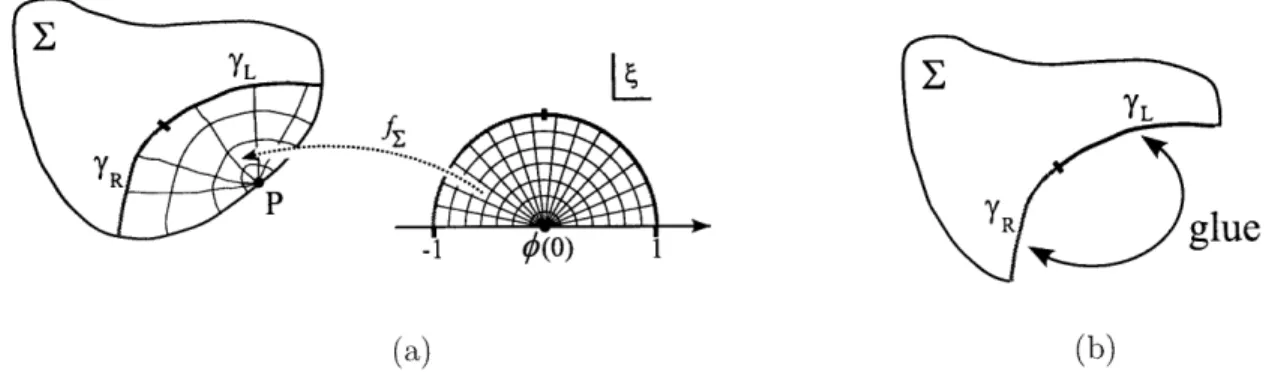
is most naturally explained for surface states.

A surface state IE) is a CFT state that is specified in terms of a Riemann surface E. See Figure 1-la. The Riemann surface has a puncture, i.e. a marked point P on its boundary. Furtheiinolc, the Riemann surface carries a coordinate patch that is specified by a map fE from the upper half unit disk to a neighborhood of the point P. The real axis is mapped to the boundary of E. Denoting the coordinate on the upper half disk by (, we thus have

fE: -+ E, f (0) = P, fr(() EOE for ER. (1.4.1)

To completely specify the state IE), it is sufficient to specify its inner product (0IE) with any state 10). Recall that, by the state-operator-correspondence, a state 10) can be associated with an operator 0. The desired inner products that specify IE) are then given by

(18)

glue

(a) (b)

Figure 1-1: (a) Illustration of a surface state IJ), defined on the Riemann surface E with a local coordinate patch around the puncture P. (b) Illustration of f E, which computes the path integral over the surface with disk topology that arises from the indicated gluing of the coordinate line.

where ([...]E denotes the path integral over the Riemann surface E, with operator insertions [...] on E. Furthermore. fz o 0(0) denotes the conformal mapping of the operator 0(0) from the ( coordinate to the Riemann surface E using fE.

More generally, we will also consider dressed surface states. These are surface states IE()) whose Riemann surface E is dressed with additional operator insertions 0. We require that all operators in 0 lie outside the coordinate patch, i.e. outside of the image of the upper half disk under fr. A dressed surface state is then completely specified by the inner products

(0, E(0)) - (f o (0) 0) . (1.4.3)

For string field theory, the midpoint of the coordinate line of a surface state, t.e. the point fr(i), plays a prominent role. It is natural to split the coordinate line along the midpoint into two parameterized curves "yL and y:

'tL(O) = _fz(e °), YR(O)= fz e i(r- )), with 0 < 0 < (1.4.4)

22

See Figure 1-la. To define the integral over a (dressed) surface state IE(O)), i.e. f E(O), we first remove the coordinate patch from the surface E, and then glue the parameterized curve

7YL(O)

to

YR(O). The resulting surface has the topology of a disk, with operator insertions 0. Then f E(O)

is simply defined as the path integral over this surface. See Figure 1-lb.

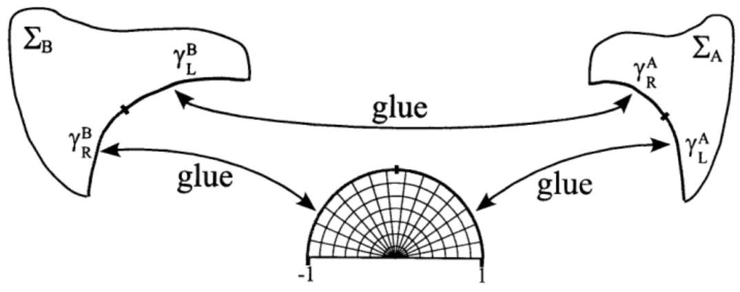
The definition of the star product EA * EB of two (possibly dressed) surface states EA and EB

is now straightforward. We remove the coordinate patches from both surface states, and glue the curve 7R(0) _{to 7L(0). The resulting surface still contains two "unglued" curves} A(0) and R (0).

We use these curves to insert a new coordinate patch. See Figure 1-2. We have thus obtained a surface with disk topology, and a new coordinate patch whose coordinate line consists of -A and

7R. We use the resulting surface state as our definition of EA * EB. Notice, that the star product

of two surface states turned out to be again a surface state.

We have now defined f and *, but the Riemann surfaces resulting from these operations are in general very complicated, and it will then not be simple to compute CFT correlators of operators

(19)

Figure 1-2: Illustration of the star product EA * EB of two surface states.

on these surfaces. We may therefore ask whether there is a frame in which these operations are natural and calculable. Such a frame indeed exists. It is the sliver frame. The sliver frame can be represented in the upper half plane z (R(z) > 0) with the coordinate patch defined through

2

f(l) = - arctan . (1.4.5) Note that the puncture P now sits at the origin in the z frame, and that YL and 7R, i.e. the left

and right half of the coordinate line, are vertical lines at R(z) = ±. The midpoint f(i) has moved off to infinity.

A natural class of surface states that can be defined in the sliver frame are the wedge states [44]. We first define the wedge surface W, as the Riemann surface that arises in the sliver frame z from the identification z _{z+ a +1. In the following, we will represent W}₀ _{in the region -} _< _(z) _{+ a,} with the vertical boundaries R(z) = -1 and R(z) = + a identified. Note that the coordinate patch defined through f () is a vertical strip of unit width on WC. The remainder of W is a strip of width a. We now define wedge states W, of width a as the surface state associated with W,:

(¢, Wa) - (f o ¢(0))W . (1.4.6)

See Figure 1-3a.

Stai multiplication of wedge states is simple - gluing two strips of width a and / to each other with the prescription above results in a strip of width a + t. Wedge states thus satisfy the simple algebra

W * Wp = W+ (1.4.7)

The wedge states of width zero, one, and infinity are of particular importance. Indeed, the wedge of vanishing width is a surface state representation of the identity string field:

W0 = 1. (1.4.8)

The wedge of unit width is nothing but the SL(2,R)-invariant vacuum:

(20)

f

f+1

-

a

-YL YR S-1

4(o)

3 -1 p(o) 1 2 2 2 2 2 2 (a) (b)

Figure 1-3: (a) Illustration of a wedge state W, of width a in the sliver frame. (b) Illustration of a Fock space state

IJp),

represented as a dressed wedge state of unit width. The path integral over the displayed surface computes the BPZ inner product (q, y9).

Finally, the wedge of infinite width is also a well-defined state in the CFT. It is the sliver state. The sliver state is a projector, i.e. it squares to itself:

Woo - lim W , Woo * W oo = Woo. (1.4.10)

a--+oo

We will be particularly interested in dressed wedge states, i.e. wedge states Wa that carry additional operator insertions O in the sliver frame:

( , Wa(0)) - (f o 0(0) O )w (1.4.11)

For example, any Fock state space Wp) associated with an operator Vp is a dressed surface state of unit width. We simply map the operator V from the origin of the upper half unit disk to the point

z = 1:

(0, P) - (f O(0) (f+l) o p(0))x (1 .4.12)

See Figure 1-3b. To see that this is the correct prescription to compute the BPZ inner product of two Fock space states q and W, notice that the maps f and f + 1 that we used precisely fill the entire wedge surface W1. This prescription thus simply glues the boundaries of the upper half disks on which q and o are defined to each other, as expected for the BPZ inner product. One particular example of the wedge representation of a Fock space state was already given above. In fact, the vacuum 10) defined in (1.4.9) is simply the Fock space state associated with the identity operator

P = 1.

Star multiplication of dressed wedge states is also simple. When we perform the gluing, we only have to be careful to translate the operator insertions to the correct position on the combined strip

Wa+.3. Defining the shift map sa(z) = z + a, we have

(0, Wa(0) * W(60)) - (f o 0(0) 0 s o (1.4.13)

Here sa o O simply shifts all operators contained in 0 by a distance a to the right so that they are correctly placed on the combined wedge of width a + i.

(21)

We have now assembled the basic ingredients necessary for our upcoming discussion of the recent analytic progress in string field theory.

1.5 The outline of this thesis

This thesis will present the results of references [13,21,33, 38]. These papers contain various analyt-ical advances in bosonic open string field theory that have been made since Schnabl's discovery of the tachyon vacuum solution. Many of these results have since been translated to open superstring field theory (see, for example, [14, 15, 17,20,23]).

In chapter 2, we present the first analytic solution of open string field theory that describes exactly marginal deformations [12, 13]. Whenever a chosen classical open string background is part of a continuously connected one-parameter family of consistent open string backgrounds, the corresponding boundary conformal field theory (BCFT) contains an exactly marginal operator V. This operator V is a conformal primary operator of dimension one, and it describes the infinitesimal deformation of the chosen background within the family of backgrounds. For such an exactly marginal deformation, we then expect a one-parameter family of solutions to open string field theory. The solutions describe the other backgrounds to which the chosen background is continuously connected. The solutions presented in chapter 2 satisfy the Schnabl gauge condition and describe

regular marginal deformations. The deformation associated with an operator V is called regular,

if operator products of V with itself do not contain any singularities. An interesting regular marginal deformation is the rollhng-tachyon solution.6 _{It describes the dynamical process of tachyon}

condensation in which an unstable D-brane starts condensing in the far past and has completely decayed into the vacuum in the far future. We study the rolling-tachyon solution in particular detail, and find that the time evolution of the tachyon field exhibits a wildly oscillating behavior. This behavior is surprising, as one might naively expect a smooth relaxation of the tachyon field to the minimum of its potential. In fact, Sen computed the time evolution of the pressure of the rolling tachyon using the BCFT boundary state, and found a smooth decay of the pressure to zero. We will reconcile these seemingly contradictory results in chapter 5, as explained below.

In chapter 3, we present a different solution of open string field theory that also describes marginal deformations [21]. This solution has the advantage that it is valid for any exactly marginal deformation. In particular, it is valid even if operator products of the marginal operator V with itself are singular. Furthermore, the solution is constructed directly from the BCFT operators which implement a change of boundary conditions along a segment of the world-sheet boundary. It thus represents a first step towards a map between consistent conformal boundary conditions (the space of BCFT's), and the space of classical solutions in open string field theory. A simple examples of an exactly marginal deformation whose operator V has singular operator products is the translation of the chosen D-brane background along a spatial direction. A physically more interesting example is the deformation from a Dp-brane to a periodic array of D(p - 1)-branes. For

6

(22)

this deformation to be exactly marginal, the periodicity of the D-branes must be a multiple of the critical radius Rc. In this case, the final array of branes has the same energy as the initial D-brane. A general solution for lower dimensional branes, i. e. the lump solution conjectured by Sen, remains an interesting open challenge of open string field theory.

The sliver frame, which plays an important role in our construction of solutions in chapters 2 and 3, also has other surprising applications. In chapter 4, we use a sliver frame analysis to show that string perturbation theory in Schnabl gauge leads to a much simpler Riemann surface geometry of tree and one-loop diagrams than in the conventional Siegel gauge or other linear b-gauges [33,45,46]. This is surprising because naively Siegel gauge seems to be the simplest possible gauge for string perturbation theory. In fact, using a Schwinger parametrization for the Siegel gauge propagators, we can build the Riemann surface associated with an amplitude simply by gluing together rectangular strips of width r. The length of the strips are given by the Schwinger parameters. Furthermore, each external state of the amplitude supplies a semi-infinite strip to the Riemann surface. Unfortunately, the assembled Riemann surface is complicated. With few exceptions, it is then impossible to conformally map the surface to a simpler region (such as the disk or the annulus) on which CFT correlators can be computed. Therefore, off-shell amplitude computations in Siegel gauge are prohibitively complicated. In chapter 4, we demonstrate that the computation in Schnabl gauge simplifies significantly. In fact, the moduli of Riemann surfaces can be exactly determined as functions of the Schnabl-gauge Schwinger parameters. In particular, the Riemann surfaces associated with tree and one-loop amplitudes can be analytically mapped to the disk and the annulus, respectively. This in principle allows the computation of arbitrary off-shell tree and one-loop amplitudes in Schnabl gauge.7

Finally, in chapter 5, we present a first step towards constructing the BCFT associated with solutions of open string field theory. An important object of every BCFT is its boundary state

IB), which encodes all closed-string point functions on a disk. Using the simplicity of

one-loop Riemann surfaces in Schnabl gauge [33], we construct an analytically calculable "string field theory boundary state" [38]. The construction is motivated by the open string field theory one-loop annulus diagram. The diagram is computed in the background of a classical solution. Surprisingly, we precisely recover the BCFT boundary state from the known wedge-based analytic solutions of open string field theory. This result is surprising, because string field theory boundai states in general only agree on-shell with the BCFT boundary state, i.e. they agree when contracted with on-shell closed string states. The precise equivalence of boundary states that we find in the computation is thus much stronger than the expected equivalence "up to BRST-exact terms". In particular, this construction is valid for the rolling tachyon solution mentioned above. We thus recover Sen's result of a smoothly decaying pressure, which is encoded in the BCFT boundary state, from the corresponding analytic solution of open string field theory, which exhibits wildly oscillating component fields. This construction of an important BCFT object from string field theory solutions thus confirms the physical interpretation of known analytic solutions and provides a nice check for the consistency of open string field theory as a whole.

7

(23)

The recent success of analytic methods for open string field theory has led to exciting progress in the field. However, many interesting open questions remain. While analytic solutions for some classical open string backgrounds were successfully constructed, a systematic prescription for the construction of solutions for a given boundary conformal field theory is still lacking. In particular, Sen's conjectured solitonic lump solution, which describes a lower-dimensional D-brane in the back-ground of a higher dimensional D-brane, has not yet been found. The opposite map, from open string field theory solutions to the space of boundary conformal field theories, has been partially established with the construction of the BCFT boundary state from known analytic solutions, but a deep understanding why this construction succeeded is still lacking.

Analytic progress in string field theory has so far been limited to open strings. It would be interesting to see whether the newly gained insights can be also be used to probe closed string physics. Closed string field theory is a manifestly non-polynomial string field theory, and its current formulation is intimately tied to the use of Siegel gauge. Overcoming these obstacles, for example by finding a new, more flexible formulation of closed string field theory would be an exciting first step. Alternatively, closed string physics may also be accessible within the framework of open string field theory. In fact, the AdS/CFT correspondence suggests that theories of open strings secretely contain a dual closed string description. It would be interesting to see how these non-perturbative degrees of freedom emerge within the framework of string field theory.

(24)

(25)

Chapter 2 Marginal deformations in Schnabl

gauge

2.1 Introduction

In this chapter we describe Schnabl gauge analytic solutions of open string field theory (OSFT) corresponding to exactly marginal deformations of the boundary conformal field theory. We closely follow the approach in [13]. Previous work on exactly marginal deformations in OSFT [47] was based on solving the level-truncated equations of motion in Siegel gauge. The level-truncated string field was determined as a function of the vacuum expectation value of the exactly marginal mode fixed to an arbitrary finite value. Level truncation lifts the flat direction, but it was seen that as the level is increased the flat direction is recovered with better and better accuracy. Instead, our approach is to expand the solution as Tx = E C AnI(n), where A parameterizes the exact flat direction.

We solve the equation of motion recursively to find an analytic expression for W(n). Our results are exact in that we are solving the full OSFT equation of motion, but they are perturbative in A; by contrast, the results of [47] are approximate since the equation of motion has been level-truncated, but they are non-perturbative in the deformation parameter.

The perturbative approach of this chapter has certainly been attempted earlier using the Siegel gauge. Analytic work, however, is out of the question because in the Siegel gauge the Riemann surfaces associated with q,(n), with n > 2, are very complicated. The new insight that makes the problem tractable is to use, as in [43], the remarkable properties of wedge states with insertions [44,48,49].

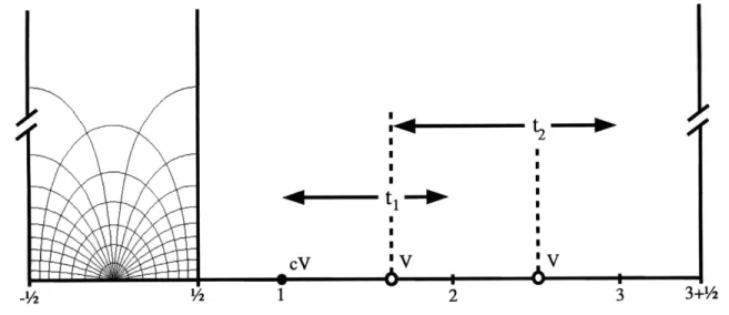
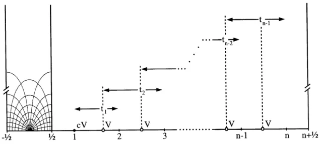
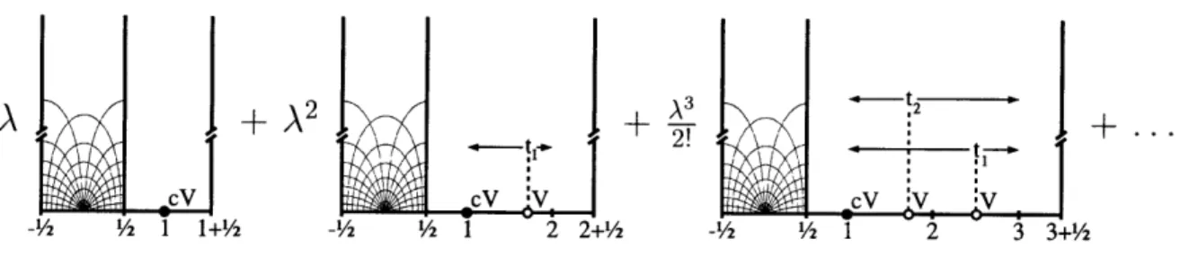
In this chapter, the matter vertex operator V that generates the deformation is assumed to have regular operator products with itself. In this case, the equation of motion can be systematically solved in the Schnabl gauge. The solution takes a strikingly compact form given in the CFT language by (2.3.3), and its geometric picture is presented in Figure 1. The solution x9(n) is made of a wedge state with n insertions of cV on its boundary. The relative separations of the boundary insertions are specified by n - 1 moduli {t}, with 0 < t, < 1, which are to be integrated over.

(26)

Each modulus is accompanied by an antighost line integral 3. The explicit evaluation of T(n) in the level expansion is straightforward for a specific choice of V.

1 X o

We apply this general result to the operator V = e 7 V [50-56]. This deformation describes a time-dependent tachyon solution that starts at the perturbative vacuum in the infinite past and (if A < 0) begins to roll towards the non-perturbative vacuum. The parameter A can be rescaled by a shift of the origin of time, so the solutions are physically equivalent. The time-dependent tachyon field takes the form

1 0 1 0

T(x) = AeJ7x + A/3n e -nx . (2.1.1)

n=2

We derive a closed-form integral expression for the coefficients /, and evaluate them numerically. We find that the coefficients decay so rapidly as n increases that it is plausible that the solution is absolutely convergent for any value of xm. Our exact result confirms the surprising oscillatory behavior found in the p-adic model [52] and in level-truncation studies of OSFT [52,56]. The tachyon (2.1.1) overshoots the non-perturbative vacuum and oscillates with ever-growing amplitude. It has been argued that a field redefinition to the variables of boundary SFT would map this oscillating tachyon to a tachyon field monotonically relaxing to the non-perturbative vacuum [56]. It would be very interesting to calculate the pressure of this exact solution and check whether it tends to zero in the infinite future, as would be expected from Sen's analysis of tachyon matter [57, 58]. We will address this question in chapter 5.

2.2 The action of B/L

2.2.1 Solving the equation of motion in the Schnabl gauge

For any matter primary field V of dimension one, the state T(1) corresponding to the operator

cV(O) is BRST closed:

QBO( 1) 0. (2.2.1)

In the context of string field theory, this implies that the linearized equation of motion of string field theory is satisfied. When the marginal deformation associated with V is exactly marginal, we expect that a solution of the form

TA)= EA n, (n) (2.2.2)

n=l

where A is a parameter, solves the nonlinear equation of motion

QB A + A * TA = 0 0. (2.2.3)

The equation that determines (n) for n > 1 is

n-1

QB ( n ) --= (n) with p(n) _ q (n-k)* _{4 '}(k) (2.2.4)

(27)

For this equation to be consistent, (D(n

) must be BRST closed. This is easily shown using the

equations of motion at lower orders. For example,

QB'1 ( 2 ) = -QB (j(1) * T(1)) = -QBI ( 1 ) * X(1) + XI(1) * QBI(1) = 0 (2.2.5) when QB"(1) = 0 . It is crucial that D(n) be BRST exact for all n > 1, or else we would encounter an obstruction in solving the equations of motion. No such obstruction is expected to arise if the matter operator V is exactly marginal, so we can determine T(n) recursively by solving QB4T(' )

= 4(n) This procedure is ambiguous as we can add any BRST-closed term to (n), so we need to choose

some prescription. A traditional choice would be to work in Siegel gauge. The solution j(n) is then given by acting with bo/Lo on j(n). In practice this is cumbersome since the combination of

star products and operators bo/Lo in the Schwinger representation generates complicated Riemann surfaces in the CFT formulation.

Inspired by Schnabl's success in finding an analytic solution for tachyon condensation, it is natural to look for a solution XPA in the Schnabl gauge:

BIA = 0. (2.2.6)

Our notation is the same as in [3, 6, 9]. In particular the operators B and L are the zero modes of the antighost and of the energy-momentum tensor T, respectively, in the conformal frame of the sliver,

Sf d f() 2

S d f() b((), L [ d T(() f() - arctan(). (2.2.7)

S27ri

f'(() 27ri f '() 7r

We define L± - L ± L* and B1 = B ± B*, where the superscript * indicates BPZ conjugation, and we denote with subscripts L and R the left and right parts, respectively, of these operators. Formally, a solution of (2.2.4) obeying (2.2.6) can be constructed as follows:

B(n)

= - (n). _(2.2.8)

L

This can also be written as

j

(n) = dT Be- T L (n), (2.2.9)

if the action of e-TL on p(n) vanishes in the limit T --+ oc. It turns out that the action of B/L on D(n)

is not always well defined. As was discussed in detail in section 4 of [13], if the matter primary field

V has a singular OPE with itself, the formal solution breaks down and the required modification

necessarily violates the gauge condition (2.2.6). On the other hand, if operator products of the matter primary field are regular, the formal solution is well defined, as we will confirm later. In the rest of this section, we study the expression (2.2.9) for n = 2 in detail.

1

Using reparameterizations, as in [9], it should be straightforward to generalize the discussion to general projectors. In this chapter we restrict ourselves to the simplest case of the sliver.

(28)

2.2.2 Algebraic preliminaries

We prepare for our work by reviewing and deriving some useful algebraic identities. For further details and conventions the reader can refer to [6,9].

An important role will e will be played by the operator L-L and the antighost analog B-B + . These operators are derivations of the star algebra. This is seen by writing the first one, for example, as a sum of two familiar derivations in the following way:

1 1 1 1 1

L -L L- L = 2 L- + I (L+ + L ) - L+ = L- + - ( L - + K) . (2.2.10) We therefore have

(L - L) (1 2) = (L - L+ ) 1 2 + 1 * (L - L+)02. (2.2.11)

Noting that L+ (01 * = L-2) + b1 * 2, we find

L(01 * .2) = L, *2+ 1 (L -L L+ ) 2, (2.2.12) B(01* 62) = BO 1 * 02 -(-1)11 * (B - B+) 2 (2.2.13)

Here and in what follows. a string field in the exponent of -1 denotes its Grassmann property: it is 0 mod 2 for a Grassmann-even string field and 1 mod 2 for a Grassmann-odd string field. From (2.2.12) and (2.2.13) we immediately deduce formulas for products of multiple string fields. For B, for example, we have

n

B(1 **- n) - (B 1)*--.* n k ( *.. (B - BL+) *... (2.2.14)

m=2

Exponentiation of (2.2.12) gives

e-TL( 4 1 * 2) e-TLo1 * e-T(L-Lt)2 . (2.2.15)

From the familiar commutators

[L, L+ ] = L+ , [B, L+] = B + , (2.2.16) we deduce

[L, L+] = L+ , [B, L+] = B+ . (2.2.17) See section 2 of [6] for a careful analysis of this type of manipulations. We will need to reorder exponentials of the derivation L - L+ . We claim that

e- T(L- L +) e(1-e - )L+ eTL (2.2.18)

The above is a particular case of the Baker-Campbell-Hausdorff formula for a two-dimensional Lie algebra with generators x and y and commutation relation [x, y] = y. In the adjoint representation we can write

0 1

(-1

(2.2.19)

(29)

It follows that as two-by-two matrices, x2 _{= x, xy}₌

y, yx = 0, and y2 = 0. One then verifies that

e x+_P y

= e(ea l)y ex when [x,y]= y. (2.2.20)

With a = -3 = -T, x = L, and y = L+ , _{(2.2.20) reproduces (2.2.18).}

2.2.3 The action of B/L and its geometric interpretation

We are now ready to solve the equation for T(2). The state T(1) satisfies

QB(1) = 0, B' (1 ) = 0, LM(1 ) = 0. (2.2.21) We will use correlators in the sliver frame to represent states made of wedge states and operator insertions. The state 9 (_{1) can be described as follows:}

(0, (1) = (f o 0(0)cV(1))w,. (2.2.22)

Note that cV is a primary field of dimension zero so that there is no associated conformal factor. Here and in what follows we use q to denote a generic state in the Fock space and 0(0) to denote its corresponding operator. The surface W, is the one associated with the wedge state W, in the sliver conformal frame. We use the doubling trick in calculating correlators. We define the oriented straight lines V,± by

V = z Re(z)= + (1 _(2.2.23)a

1 1 (2.2.23)

orientation: (1 + a) - i 00 - - (1 + ) + i .

2 2

The surface We can be represented as the region between Vo and V2, where Vo and V2 are

identified by translation.

A formal solution to the equation QB x(2) = -(1) * (1) is

qj(2) = - dT Be-TL [ (1) * q (1)] . _(2.2.24)

By construction, B4 (2) _{= 0. Using the identities (2.2.15) and (2.2.13), we have}

qj,(2) dT [B eTL j(1l) -= e-T(L -L) p(1) _ e-TL (1) (B B) e-T(L-L+L) (1).

(2.2.25)

Because of the properties of M(1) in (2.2.21), the first term vanishes and the second reduces to

j2)

T,( ()dT * (B - B)) (1) (2.2.26) We further use the identity (2.2.18) together with L( 1 _{) = 0 to find}

(2= dT ,() (B - Bj) e(1- )L '(1) . (2.2.27)

(30)

It follows from [B, L = B+ that [B, g(L/)] = B g'(LL) for any analytic function g. Using this

formula with BI( 1) = 0, we find

41(2) = dT e- (1) * e(-e- )L+ B+(1) (2.2.28)

Using the change of variables t = e- T , we obtain the following final expression of 4(2): S((2)

j

(dt1

e

) (- + T(1) (2.2.29) 0

There is a simple geometric picture for 4(2). Let us represent ( 0, X(2) ) in the CFT formulation. The exponential action of L+ on a generic string field A can be written as

e- LA = e- L+ ( * A) = e- L + A = W * A. (2.2.30)

Here we have recalled the familiar expression of the wedge state W =- e L+ = e-aLiZ [43], where I is the identity string field. We thus learn that e- LL with a > 0 creates a semi-infinite strip with a width of a in the sliver frame, while e-aLt with a < 0 deletes a semi-infinite strip with a width of

lal.

The inner product ( , 4(2) ) is thus represented by a correlator on W/2_lt-1 = l+t.

In other words, the integrand in (2.2.29) is made of the wedge state Wl+t with operator insertions. The state 0 is represented by the region between Vo- and V+ with the operator insertion f o 0(0) at the origin. The left factor of (1) in (2.2.29) can be represented by the region between Vo+ and V2+

with an insertion of cV at z = 1. For t = 1 the right factor of (1) can be represented by the region between V+ and V+ with an insertion of cV at z = 2. For 0 < t < 1, the region is shifted to the one between V2 t -1 V+ and V = V2+ 2t, and the insertion of cV is at z = 2 - t - 11 = 1 + t.

2-21t-11- 2t 4-21t-11- 2+2t,

Finally, the operator (-B + ) is represented by an insertion of 3 [9] defined by

B

=

dz b(z), (2.2.31)

where the contour of the integral can be taken to be -V +" with 1 < ca < 1 + 2t. We thus have

(,(2) )= dt (f o (0)cV(1)B1cV(1 + t)) . (2.2.32) As t - 0 the pair of cV's collide, and at t = 1 they attain the maximum separation.

The state 4(2) should formally solve the equation of motion by construction. Let us examine the BRST transformation of 4(2) more carefully based on the expression (2.2.32). The BRST operator in ( , QBT) can be represented as an integral of the BRST current on V2+t)

-

V

2

(4, QB j(2)) dt

f

o (0) 2jB(z) cV(1) B cV(l+ t) (2.2.33)

-V + V2 +t)

2

To derive this we first use the relation ( ,QB I(2) = _(_B1) , " I'(2)), where QB on the right-hand side is an integral of the BRST current jB over a contour that encircles the origin counterclockwise, with the operator

3B placed to the left of f o 0(0) in the correlator. Using the identification of the surface Wl+t, the contour can be

deformed to -V2,+t) + VO+.In the correlator, we move the BRST current from the left of f o q(0) to the right of it. This cancels (-1)0, and the additional minus sign is canceled by reversing the orientation of the contour.

(31)

where JB _{is the BRST current. Since cV is BRST closed, the only nontrivial action of the BRST}

operator is to change the insertion of the antighost to that of the energy-momentum tensor:

( q, QBp (2)) = - dt (f o (O) cV(1) C cV(1 + t) )w,+ , (2.2.34)

where

C

dz T(z),

(2.2.35)

27rid

and the contour of the integral can be taken to be -V +_{f with 1 < a < 1 + 2t. The minus sign on}

the right-hand side of (2.2.34) is from anticommuting the BRST current with the left cV. Since

at e- t L + = -L e- t L+ and -LL corresponds to

L

in the correlator, an insertion of

L

is equivalent to taking a derivative with respect to t [3]. We thus find

(0, QBI (2

) -j dt a(fo (O) cV(1) cV(1 + t) )w,,, . (2.2.36)

The surface term from t = 1 gives - (1) * (1). The equation of motion is therefore satisfied if the surface term from t = 0 vanishes. The surface term from t = 0 vanishes if

lim cV(O) cV(t) = 0. (2.2.37)

t--0

Therefore, j(2) _{defined by (2.2.32) does solve the equation QBT(2) + qj(1) ,(1)} _{= 0 when V}

satisfies (2.2.37). Since 9(1) * _{T(1) is a finite state, the equation guarantees that QB (}2_{) is also}

finite. However, it is still possible that T(2) has a divergent term which is BRST closed. The ghost part of Xp (2) is finite since it is given by an integral of 7bt over t from t = 0 to t = 1, where Vn, is the key ingredient in the tachyon vacuum solution [43]:

( 0, On ) = (f o 0(0) c(1) Bc(1 + n) )wl+n, (2.2.38)

and the contour of the integral for B can be taken to be -V, with 1 < a < 2n + 1. When the operator product of V with itself is regular, the condition (2.2.37) is satisfied and ij(2) itself is finite. Note that V(0) V(t) in the limit t -- 0 can be finite or can be vanishing. We construct

1

(n)

for marginal operators with regular operator products in the next section. When the operator

product of V with itself is singular, the formal solution I(2) is not well defined. We postpone the discussion of marginal solutions with singular operator products to chapter 3.

2.3 Solutions for marginal operators with regular operator

prod-ucts

In the previous section we constructed a well-defined solution to the equation QB4 (2 )

+ I (1) * qIf(1)

0 when V has a regular operator product. In this section we generalize it to T(n) for any n. We then present the solution that corresponds to the decay of an unstable D-brane in §2.3.2.

Analytic progress in open string field theory

Analytic progress in open string field theory

Michael Stefan Kiermaier

AUG 0 4 2009

Submitted to the Department of Physics

LIBRARIES

in partial fulfillment of the requirements for the degree of

Doctor of Philosophy

ARCHIVE

at the

MASSACHUSETTS INSTITUTE OF TECHNOLOGY

June 2009

@

Massachusetts Institute of Technology 2009. All rights reserved.

Author ...

...

Department of Physics

May 20, 2009

Certified by ...

Barton Zwiebach

Professor of Physics

Thesis Supervisor

Accepted by ...

Thomas J. Greytak

Lester Wolfe Professor of Physics, Associat eDepartment Head for Education

Analytic progress in open string field theory

by

Abstract

Acknowledgments

Contents

Chapter 1

Introduction

1.1

From string theory to string field theory

N

1.2

Sen's conjectures

1.3

Witten's cubic open string field theory

QXF

'F

= T

+ Qx

(1.3.2)

(x

Q4)

(.,

24

*

+ 3

T*4*X

a

:

-*K,

:

-C.

(1.3.9)

(A,

Q

*

f:

*

Q

SX

x

x

T

1.4

Surface states, star products, and the algebra of wedge states

f

glue

7YL(O)

f

f+1

a

4(o)

IJp),

1.5

The outline of this thesis

Chapter 2

**T4X**