The combinatorics of adinkras

The Combinatorics of Adinkras

by

Yan Zhang

Submitted to the Department of Mathematics

A\CH!VES

MASSACHUi;T~ , ST[ Yt1j . LU.....

"-~~R

?RA

EJS

in partial fulfillment of the requirements for the degree of

Doctor of Philosophy

at the

MASSACHUSETTS INSTITUTE OF TECHNOLOGY

June 2013

@

Massachusetts Institute of Technology 2013. All rights reserved.

Author ...

.

..

...

Departmeit'of Iathematics

April 23, 2013

Certified by

...

Richard Stanley

Professor

Thesis Supervisor

Accepted by...

Michel Goemans

Chairman, Department Committee on Graduate Theses

The Combinatorics of Adinkras

by

Yan Zhang

Submitted to the Department of Mathematics

on April 23, 2013, in partial fulfiliment of the

requirements for the degree of Doctor of Philosophy

Abstract

Adinkras are graphical tools created to study representations of supersymmetry

al-gebras. Besides having inherent interest for physicists, the study of adinkras has already shown nontrivial connections with coding theory and Clifford algebras. Fur-thermore, adinkras offer many easy-to-state and accessible mathematical problems of algebraic, combinatorial, and computational nature. In this work, we make a self-contained treatment of the mathematical foundations of adinkras that slightly generalizes the existing literature. Then, we make new connections to other areas including homological algebra, theory of polytopes, Pfaffian orientations, graph col-oring, and poset theory. Selected results include the enumeration of odd dashings for all adinkraizable chromotopologies, the notion of Stiefel-Whitney classes for codes and their vanishing conditions, and the enumeration of all Hamming cube adinkras up through dimension 5.

Thesis Supervisor: Richard Stanley Title: Professor

Acknowledgments

First and foremost, I thank Sylvester "Jim" Gates for teaching the subject to me. This project delves into many areas of mathematics - being not an expert in any of them I am very lucky to have had people help me with every subject. I thank Brendan Douglas, Greg Landweber, Kevin Iga, Richard Stanley, Alex Postnikov, Henry Cohn, Joel Lewis, and Steven Sam for helpful general discussions. I thank Yi Sun for brushing up my complex analysis and the use of Laplace's Method. Anatoly Preygel, Nick Rozenblyum, and Josh Batson gave me very enlightening lessons in algebraic topology and made the relevant sections possible. I am especially grateful to Tristan Hiibsch for his unreasonably generous gift of time and patience through

countless communications.

I want to re-thank Richard Stanley, Alex Postnikov, and Henry Cohn for being my thesis committee and for having helpful conversations. In particular, I am deeply grateful for the advice and support throughout my studies that Richard has given me, especially through my more idiosyncratic and more difficult times.

Contents

1 Introduction

1.1 Posets . . . .

1.2 Chromotopologies and Adinkras . . . .

1.3 Multigraphs . . . . 1.4 Physical Motivation . . . . 2 The 2.1 2.2 2.3 Classification Theorems

Graph Quotients and Codes . . . . . Clifford Algebras and Codes . . . . . The Classifications . . . . 3 Dashings 3.1 A Homological View 3.2 3.3 3.4 3.5 3.6

Generalizations and Sightings of Odd Dashings . Even Dashings . . . .

Decomposition and Dashings on Hamming Cubes Dashings on Adinkras . . . .

A Generalization of Dashings and Noneven Grap

4 Stiefel-Whitney Classes of Codes

4.1 Seeing Codes as Maps . . . .

4.2 Prelim inaries . . . .

4.3 Interpretation of Vanishing Stiefel-Whitney Classes

5 Rankings

5.1 Preliminaries: Hanging Gardens . . . .

5.2 The Rank Family Lattice . . . .

5.3 Counting Rankings of the Hamming Cube . . . . . 5.4 Grid Graphs and Eulerian Orientations . . . .

5.5 Rankings and Discrete Lipschitz Functions . . . . .

5.6 Discrete Lipschitz Functions and Dashings . . . . .

5.7 Rankings and Colorings . . . .

9 . .10 . .10 . .13 . . 13 17 17 19 21 23 . . . . 23 . . . . 24 . . . . 25 . . . . 26 . . . . 29 .. ... 31 33 . . . . 33 . . . . 35 . . . . 37 43 . . . . 44 . . . . 46 . . . . 50 . . . . 51 . . . . 53 . . . . 58 . . . . 58 s

6 Physics and Representation Theory 61

6.1 Constructing Representations . . . . 61

6.2 When are Two Adinkras Isomorphic? . . . . 62

6.3 Clifford Representations . . . . 64

Chapter 1

Introduction

In a series of papers starting with

1151,

different subsets of the "DFGHILM collabora-tion" (Doran, Faux, Gates, Hibsch, Iga, Landweber, Miller) have built and extended the machinery of adinkras. Following the ubiquitous spirit of visual diagrams in physics, adinkras are combinatorial objects that encode information about the rep-resentation theory of supersymmetry algebras. Adinkras have many intricate links with other fields such as graph theory, Clifford theory, and coding theory. Each of these connections provide many problems that can be compactly communicated to a (non-specialist) mathematician. This work is a humble attempt to bridge the language gap and generate communication.

In short, adinkras are chromotopologies, a class of edge-colored bipartite graphs, with two additional structures, a dashing condition on the edges and a ranking condi-tion on the vertices. In this chapter, we give the preliminaries, including a discussion of physical motivation in Section 1.4. We then redevelop the foundations in Chapter 2 in a slightly different way from the existing literature, leading to a cleanly-nested set

of classifications (Theorems 2.3.1, 2.3.2, and 2.3.3).

After this semi-expository portion, we look at the two aforementioned condi-tions, dashings and rankings, separately. For each condition, we extract the purely combinatorial problem, make connections with different area of mathematics, and generalize the corresponding notion to wider classes of graphs.

In Chapter 3 we use homological algebra to study dashings; our main result is the enumeration of odd dashings for any chromotopology. We also make a connection with the theory of Pfaffian orientations. In Chapter 4, we introduce the idea of Stiefel-Whitney classes of codes, a concept inspired by the combination of dashings and topology.

After dashings, we study rankings. In Chapter 5, we use the theory of posets to put a lattice structure on the set of all rankings of any bipartite graph (including chromotopologies); we also count Hamming cube rankings up through dimension 5. After these enumerative results, we introduce the strongly-related concept of discrete

Lipschitz functions and make some connections between rankings and the theory of

These chapters focus on combinatorics and not as much on the foundational prob-lems of adinkras from the physics literature. We return to these roots in Chapter 6, ending with a quick survey of recent developments and some original observations.

1.1

Posets

We assume basic notions of graphs. For a graph G, we use E(G) to denote the edges of G and V(G) to denote the vertices of G. We also assume most basic notions of posets (there are many references, including [38]).

One slight deviation from literature is that we consider the Hasse diagram for a poset as a directed graph, with x -+ y an edge if y covers x. Thus it makes sense

to call the maximal elements (i.e. those x with no y > x) sinks and the minimal

elements sources.

For this work, a ranked poset is a poset A equipped with a rank function h: A -+ Z

such that for all x covering y we have h(x) = h(y)+1. There is a unique rank function

ho among these such that 0 is the lowest value in the range of ho, so it makes sense to define the rank of an element v as ho(v). The largest element in the range of ho is then the length of the longest chain in A; we call it the height of A. We remark that such a poset is often called a graded poset, though there are similar but subtly different uses of that name. Thus, we use ranked to avoid ambiguity.

1.2

Chromotopologies and Adinkras

An n-dimensional chromotopology is a finite connected simple graph A such that the following conditions hold:

" A is n-regular (every vertex has exactly n incident edges) and bipartite.

Re-specting the physics literature, we call the two sets in the bipartition of V(A)

bosons and fermions. As the actual choice is mostly arbitrary for our purposes,

we will usually not explicitly include this data.

" The elements of E(A) are colored by n colors, which are elements of the set

[n] = {1, 2, ... , n} unless denoted otherwise, such that every vertex is incident

to exactly one edge of each color.

" For any distinct i and

j,

the edges in E(A) with colors i and

j

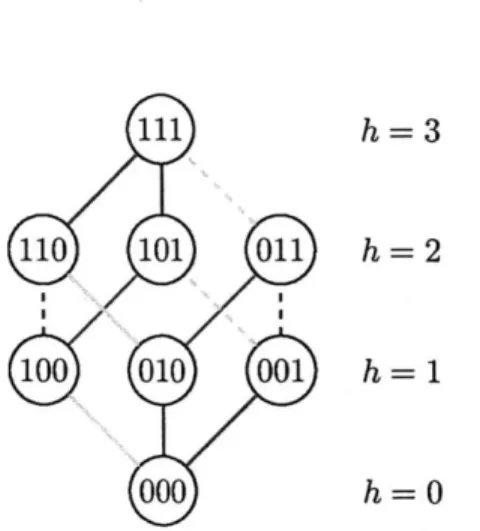
form a disjoint union of 4-cycles.

We now introduce the key example of a chromotopology. Define the n-dimensional

Hamming cube I" to be the graph with 2n vertices labeled by the n-codewords, with

an edge between two vertices if they differ by exactly one bit. It is easy to see that In is bipartite and n-regular. Noticing that I = 11 is just a single edge, our exponentiation In is justified as a cartesian product. Now, if two vertices differ

at some bit i, 1 < i < n, color the edge between them with the color i. The

2-colored 4-cycle condition holds, so we get a chromotopology that we call the

n-cubical chromotopology I. Figure 1-1 shows I3.

100 - 000

101 - 001

110 010

111 -011

Figure 1-1: The 3-cubical chromotopology I. We can take the bosons to be either

{000, 011,101, 1101 or {001, 010, 100, 111} and take the fermions to be the other set.

We now define two structures we can put on a chromotopology.

1. let a ranking of a bipartite graph (in particular, any chromotopology) A be a

map h : V(A)

-+

Z that gives A the additional structure of a ranked poset on

A via h as the rank function. By this, we mean that we identify A with the

Hasse diagram of the said ranked poset with rank function h. We consider two

rankings equivalent if they differ only by a translate, as the resulting ranked

posets would then be isomorphic. Given a ranking h of A, we say that A is

ranked by h.

In this work, such as in Figure 1-3, we will usually represent ranks via vertical

placement, with higher values of h corresponding to being higher on the page.

The vertices at the odd ranks and the vertices at the even ranks naturally form

the bipartition of V(A).

Any bipartite graph (and thus any chromotopology) A can be ranked as follows:

take one choice of bipartition of V(A) into bosons and fermions. Assign the

rank function h to take values 0 on all bosons and 1 on all fermions, which

creates a ranked poset with 2 ranks. We call the corresponding ranking a

valise. Because we could have switched the roles of bosons and fermions, each

bipartite graph gives rise to exactly two valises. For an example, see Figure 1-2.

We remark that in the existing literature, such as [9], posets are never

men-tioned and the following equivalent definition is used, under the names

engi-neerable or non-escheric: give A the structure of a directed graph, such that

in traversing the boundary of any (non-directed) loop with a choice of

direc-tion, the number of edges oriented along the direction equals the number of

edges oriented against the direction. This is easily seen to be equivalent to our

definition.

2. let a dashing of a bipartite graph A be a map d: E(A) -+ Z2 (in this work, we

will always use Zk as shorthand to denote Z/kZ). Given a dashing d of A, we say that A is dashed by d. We visually depict a dashing as making each edge

e E E(A) either dashed or solid, corresponding to d(e) = 1 or 0 respectively.

We will slightly abuse notation and write d(v, w) to mean d((v, w)), where

(V, w) is an edge from v to w.

For a chromotopology A, a dashing is an odd dashing if the sum of d(e) as e runs over each 2-colored 4-cycle (that is, a 4-cycle of edges that use a total of 2 colors) is 1 E Z2 (alternatively, every 2-colored 4-cycle contains an odd

number of dashed edges). If A is dashed by an odd dashing d, we say that A is well-dashed.

100 ill 001 010

110 101 011 000

Figure 1-2: A valise; one possible ranking of the chromotopology If.

An adinkra is a ranked well-dashed chromotopology. We call a graph that can be made into an adinkra adinkraizable. Since any chromotopology, being a bipar-tite graph, can be ranked, adinkraizability is equivalent to the condition of having at least one odd dashing. A well-dashed chromotopology is just an adinkraizable chromotopology equipped with this dashing.

We frequently use some forgetful functions in the intuitive way: for example, given any (possibly ranked and/or well-dashed) chromotopology A, we will use "the chromotopology of A" to mean the underlying edge-colored graph of A, forgetting the ranking and the dashing.

Many of our proofs involve algebraic manipulation. To make our treatment more streamlined, we now set up algebraic interpretations of our definitions.

" The condition of A being a chromotopology is equivalent to having a map

qi: V(A) -+ V(A) for every color i that sends each vertex v to the unique vertex

connected to v by the edge with color i, such that the different qi commute

(equivalently, the qj generate a Z' action on V(A). The well-definedness of the

qi corresponds to the edge-coloring condition and the commutation requirement

corresponds to the 4-cycle condition. Note that qj is an involution, as applying

qj twice simply traverses the same edge twice. Furthermore, qi sends any boson

to a fermion, and vice-versa.

" The condition of a chromotopology A being well-dashed (with dashing

func-tion d) is equivalent to having the maps 'q anticommute, where we define

111

h = 3

110

101

011

h=2

010

001

h=

1

000

h=

0

Figure 1-3: An adinkra with the chromotopology

I.

1.3

Multigraphs

It seems natural to extend our definition to multigraphs. Let a multichromotopology

be a generalization of chromotopology where we relax the condition that the graph

be simple and now allow loops and multiple-edges. The n-regular condition remains,

but is reinterpreted so that a loop counts as degree 1 as opposed to 2. The algebraic

condition is still that the qi must commute. However, the combinatorial version of

the rule (that the union of edges of different colors i and

j

form a disjoint union of

4-cycles) must be extended to allow degenerate 4-cycles that use double-edges or loops.

Define the well-dashed and ranked properties on multichromotopologies analogously,

again extending our condition for 2-colored 4-cycles to allow double-edges and loops.

These generalizations- exclude each other in a cute way:

" While there are ranked multichromotopologies with double-edges, no

well-dashed multichromotopology can have a double-edge because a double-edge

immediately gives a degenerate 2-colored 4-cycle, and it is impossible for the

sum of dashes over a degenerate 2-colored 4-cycle to be odd.

" The loops have the opposite problem: they allow new well-dashed

multichro-motopologies, but none of these multichromotopologies can be ranked because

bipartite graphs cannot have loops.

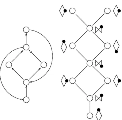
See Figure 1-4 for some examples.

The above discussion shows that the natural definition of multiadinkras, that

is, well-dashed ranked multichromotopologies, does not give us any new objects that

are not already adinkras. However, multigraphs naturally appear in our classification

paradigm in Chapter 2, so they are still a nice notion to have for our work.

0

Figure 1-4: A ranked multichromotopology (with double-edge) that cannot be well-dashed, and a well-dashed multichromotopology (with loops) that cannot be ranked.

The reader is equipped to understand the rest of the paper (with the exception of Chapter 6) with no knowledge from this section. However, we hope our brief outline will serve as enrichment that may provide some additional intuition, as well as provide a review of the original problems of interest (where much remains to be done). While knowledge of physics will help in understanding this section, it is by no means necessary. We have neither the space nor the qualification to give a comprehensive review, so we encourage interested readers to explore the original physics literature.

The physics motivation for adinkras is the following: "we want to understand off-shell representations of the N-extended Poincar6 superalgebra in the 1-dimensional worldline." There is no need to understand what all of these terms mean' to ap-preciate the rest of the discussion; we now sketch the thinking process that leads to

adinkras.

Put simply, we are looking at the representations of the algebra poll' generated

by N

+

1 generators Qi, Q2, ... , QN (the supersymmetry generators) and H = iOt

(the Hamiltonian), such that

{QI, QJ} = 261jH,

[Q1, H] =0.

Here, 6 is the Kronecker delta, {A, B} = AB + BA is the anticommutator, and

[A, B] = AB - BA is the commutator. We can also say that pollN is a superalgebra

where the Qi's are odd generators and H is an even generator. Since H is basically a time derivative, it changes the engineering dimension (physics units) of a function

f

by a single power of time when acting on

f.

Consider R-valued functions {#1,...,qm} (the bosonic fields or bosons) and

{$1,..., m} (the fermionic fields or fermions), collectively called the component

fields. The fact that the two cardinalities match come from the physics assumption

that the representations are off-shell; i.e. the component fields do not obey other differential equations. We want to understand representations of pollN acting on the following infinite basis:

{Hkq#, HkV# I k E N; I, J < m}.

There is a subtlety here, as these infinite-dimensional representations are frequently called "finite-dimensional" by physicists, who would just call the

{#O}

and the {OI} as the "basis," emphasizing the finiteness of m. A careful treatment of this is given

in [11].

In particular, we want to understand representations of polN satisfying some physics restrictions (most importantly, having the supersymmetry generators send bosons to only fermions, and vice-versa; this kind of "swapping symmetry" is what supersymmetry tries to study). We restrict our attention to representations where

the supersymmetry generators act as permutations (up to a scalar) and also possibly the Hamiltonian H = iD,, on the basis fields: we require that for any boson 0 and

any

_Q1,

Qjq = ±(-iH)p = t8),

where s E {0, 1}, the sign, and the fermion

V

depends on

#

and I. We enforce a similar requirement

QJ0= ±i(-iH)8 o =

(at)'#

for fermions. We call the representations corresponding to these types of actions

adinkraic representations. For each of these representations, we associate an adinkra.

We now form a correspondence between our definition of adinkras in Section 1.2 and our definition for adinkraic representations.

adinkras representations

vertex bipartition bosonic/fermionic bipartition

colored edges and q, action of

Q,

without the sign or powers of (-iH) dashing

/

sign in

41

sign in

Q,

change of rank by q, and 71 powers of (-iH) in

Q,

ranking partition of fields by engineering dimension

To summarize,

An adinkra encodes a representation of polN. An adinkraic representation is a representation of po'lN that can be encoded into an adinkra.

Our main problem is then the following:

Problem 1. What are all the adinkraic representations of pol1N 7

One motivation for the restriction of study to adinkraic representations is having an easily-visualized graphical tool to study these representations; another is that the set of adinkraic representations is already rich enough to contain representations of interest. When the poset structure of our adinkra A is a boolean lattice, we get the classical notion of superfield introduced in [351 by Salam and Strathdee. When the poset of A is a height-2 poset (in which case we say that A is a valise), we get [12]'s Clifford supermultiplet. By direct sums, tensors, and other operations familiar to the Lie algebras setting, it is possible to construct many more representations, a technique that has been extended to higher dimensions in [26].

Chapter 2

The Classification Theorems

We now classify multichromotopologies, chromotopologies, and adinkraizable chro-motopologies; we also note the pleasant connections with codes and Clifford algebras that make adinkras fascinating. Compared to the relevant sections of the original literature, our approach is more general and at times more compact, though we owe most ideas in this chapter to the original work.

2.1

Graph Quotients and Codes

In this section, we recover the main result (Theorem 2.3.3) classifying adinkraizable chromotopologies from the existing literature. However, our more general approach (using multigraphs) gives the benefit of easily obtaining classification theorems of multichromotopologies and chromotopologies that are very analogous in flavor.

We now give a quick review of codes (there are many references, including [27]).

An n-codeword is a vector in Z, which we usual write as bib2 ... bn, bi E Z2. We

distinguish two n-codewords In = 11... 1 and 0, = 00... 0, and when n is clear

from context we suppress the subscript n. The number of l's in a codeword v is called the weight of the string, which we denote by wt(v). We use i to denote the bitwise complement of v, which reverses O's and l's. For example, 00101 = 11010.

An (n, k)-linear binary code (for this work, we will not talk about any other kind of codes, so we will just say code for short) is a k-dimensional Z2-subspace of codewords.

A code is even if all its codewords have weight divisible by 2 and doubly even if all

its codewords have weight divisible by 4.

Consider the n-cubical chromotopology Ic. For any linear code L C Zn, the quotient Z'/L is a Z2-subspace. Using this, we define the map PL, which sends Ign

to the following multichromotopology, which we call the graph quotient (or quotient for short) I"/L:

* let the vertices of Ic/L be labeled by the equivalence classes of Z'/L and define

the preimage over every vertex in I,/L contains 2k vertices, so

I,/L

has 2n-k

vertices.

* let there be an edge pL(v, w) in I4'/L with color i between pL(v) and pL(w) in

I'/L if there is at least one edge with color i of the form (v', w') in Z', with

v' E pZL(v) and w' E pL1(w).

Every vertex in I,/L still has degree n (counting possible multiplicity) and the commutivity condition on the qi's is unchanged under a quotient, so I"/L is indeed a multichromotopology. Denote its underlying multigraph by I'/L. We now prove some properties of the quotient.

Proposition 2.1.1. The following hold for A = In

/L:

1. A has a loop if and only if L contains a codeword of weight 1; A has a double

edge if and only if L contains a codeword of weight 2. Thus, A is a simple graph if and only if L contains only codewords of weight 3 or greater.

2. A can be ranked if and only if A is bipartite, which is true if and only if L is an even code.

Proof. 1. Suppose A has a loop. This means some edge (v, w) in I" has both

endpoints v and w mapped to the same vertex in the quotient. Equivalently,

(v - w) E L. However, v and w differ by a codeword of weight 1. Suppose A

has a double edge (v, w) with colors i and j. Since q1(q2(v)) = v in A = I"/L,

for some v' E pL1(v), we must have in In that qi(q2(v')) - v' is in L. But this

is a weight 2 codeword with support in i and j. The logic is reversible in both of these situations.

2. Suppose A were not bipartite, then A has some odd cycle. One of the preimages of this cycle in In is a path of odd length from some v to some w that both map to the same vertex under the quotient (i.e. v - w E L). Since each edge

changes the weight of the vertex by 1 (mod 2), v - w must have an odd weight.

Since v - w E L, L cannot be an even code. For the other direction, note that

if L were an even code such odd cycles cannot occur.

Recall that any bipartite graph can be ranked by making a valise. If A can be ranked via a rank function h, the sets {v E V(A) I h(v) - 0 (mod 2)} and

{v E V(A) I h(v) a 1 (mod 2)} must be a bipartition of A because all the

edges in A change parity of h.

The most difficult condition to classify is being well-dashed, which is intricately connected with Clifford algebras. We focus on them in the next section.

2.2

Clifford Algebras and Codes

For our purposes, the Clifford algebra is an algebra C1(n) with generators ft, ... ,

and the anticommutation relations

{yiyj} =2J, -1.

The Clifford algebra can be defined for any field, but we will typically assume R. There are also more general definitions than what we give, though we won't need them for our paper. For references, see [1] or [7].

We can associate an element of the Clifford algebra to any n-codeword b = b1b2 ... bn, by defining

clif(b) =

where the product is taken in increasing order of i. Call these elements monomials. The 2n possible monomials form a basis of C1(n) as a vector space, and the 2n+1

signed monomials ± clif(b) form a multiplicative group SMon(n), or just SMon when the context is clear. It is easy to see that two signed monomials of degrees

a and b commute if and only if ab = 0 (mod 2), and one could equivalently define

Clifford algebras as commutative superalgebras with odd and even parts generated

by the odd and even degree monomials, respectively.

The following facts are needed for Proposition 2.2.4, where we defined the notion of an almost doubly-even code as a code with all codewords having weight 0 or 1

(mod 4).

Lemma 2.2.1. For any two codewords w1 and w2 in an almost doubly-even code,

we have

(wi - W2) + wt(wi) wt(w2) = 0 (mod 2), where the first term is the dot product in Z2.

Proof. Given an almost doubly-even length n code L, introduce 3 new bits in the

code to construct a doubly-even length (n + 3) code L' via the following map g: for

w E L, let g(w E L) be the concatenation wJ111 if w has odd weight and w|000 if w has even weight. Since the weight parity of two codewords are additive modulo

2, g(v

+

w) = g(v)

+

g(w) and L' is linear. Our construction also clearly ensures

that L' is doubly-even. It is well known (see, for example, [27]) that doubly-even codes are self-orthogonal, so (g(wi) - g(W₂)) = 0 (mod 2) for all w, and W₂ in L. But

(9(W1) .g(W2)) - (WI -W2) is 0 (mod 2) when either w, or w2 has even weight (because

the additional bits 000 cannot affect the dot product) and is 1 (mod 2) exactly when both w, and W_{2 have odd weights. This is equivalent to the condition we want to}

prove. l

Lemma 2.2.2. The image of a code L under clif is commutative if and only if for all a,b E L,

In particular, an almost-doubly-even code satisfies this property.

Proof. Finally, consider clif (a) = a ... ,.Yar and clif(b) = -y'b . . ., where r = wt(a)

and s = wt(b). Note we can get from clif (a) clif(b) to clif(b) clif(a) in wt(a) wt(b)

transpositions, where we move, in order -b,, - - - , 7yb through clif (a) to the left, picking

up exactly wt(a) powers of (-1). However, we've also overcounted once for each time a and b shared a generator 7yj, since -yj commutes with itself. Therefore, we have exactly (a -b) + wt(a) wt(b) powers of (-1). The condition for commutativity is then that this quantity be even for all pairs a and b. E

These concepts of almost-doubly-even codes and commuting codewords have ap-peared independently in the undergraduate thesis work of Ratanasangpunth [34], where the commutation condition defines a class of codes called Clifford codes. Ratanasangpunth goes forth to prove further structural and classification theorems for these codes.

Proposition 2.2.3. A code L is an almost doubly-even code if and only if L has the property that for a suitable sign function s(v) E {±1} with s( 0) = 1, the set

SMonL = {s(v) clif(v) v c L} form a subgroup of SMon.

Proof. Without loss of generality, say clif(v) = s(v)y 1 i. Then

clif(v)2 = (717-2 - -7k)QY17Y2 - -qk)

= (-1)(k-1) (72 73 -. -0 - (71) 7172 - -- k)

= (-1)k(k-1)/2

Suppose s exists. Then, we must not have (-1) E SMonL (since we already have 1 z SMonL. Therefore, it is necessary to have the last quantity equal 1, which happens exactly when wt(v) = 0 or 1 (mod 4) for all v E L.

If L were an almost-doubly even code, then pick a basis

l,...

, lk of L and assign

s(li) = 1 for all i. Note by the above equations clif(l) 2 = 1 for all i. The linear independence of the li is equivalent to the condition that no group axioms are broken

by this choice of li. Now, we can extend the definition to

s(J clif(1j)) = J7 s(7J(clif(li)),

iEI iEI

which is well-defined and closed under multiplication since the li commute and square

to 1. L

Let an almost-doubly even code be a code where all codewords in the code have weight 0 or 1 (mod 4). The following result extends the ideas used in proving [12, Theorem 4.4].

Proposition 2.2.4. The multichromotopology A = I,/L can be well-dashed if and only if L is an almost doubly-even code.

Proof. Given a codeword v = v1v2 . .. vn, define qv to be the map ; -.

Suppose we have an odd dashing. Let v and w be codewords in L. Both qv and i, take any vertex to itself in R[V(A)] with possibly a negative sign, since the _q are basically the qj with possibly a sign, and following a sequence of qj corresponding

to a codeword is a closed loop in I,/L. This means q, and q, must commute;

furthermore, q2, must be the identity map for any v E L. By Lemma 2.2.2, this is

exactly the condition required for L being an almost-doubly even code.

Now, suppose L were an almost doubly-even code. Then by Proposition 2.2.3, we can find a sign function s such that {s(v) clif(v) I v E L} form a subgroup

SMonL C SMon, the signed monomials of Cl(n). This gives a well-defined action

of SMon on SMon/SMonL via left multiplication while possibly introducing signs. The cosets of SMonL under SMon naturally correspond to V(A), so we can define

qi(v) to introduce the same sign as -yj on clif(v) E SMon/SMonL. Since we have a Clifford algebra action, we get the desired anticommutation relations between qj and thus an odd dashing.

2.3

The Classifications

In this section, we give three nested classification theorems for three nested types of codes.

To start, recall that quotients of I' are multichromotopologies. Surprisingly, the converse is also true, which gives us our main classification:

Theorem 2.3.1. Multichromotopologies are exactly quotients Ig/L for some code L.

Proof. Take a multichromotopology A. Consider the abelian group G acting on V(A)

generated by the qj. The elements of G can be written as g = q" q 2 _{... qnT, where}

Si E Z2 for all i. Consider the isomorphism q: G -+ L which sends such a g to the

n-codewords S1s2 ... s-n E Zn. Take any vertex vo E V(A) and consider its stabilizer

group H under G. O(H) is a subspace of Zn and thus must be some code L. Any vertex v is equal to g(vo) for some g E G, so we may label v with the coset O(g) + L. It is easy to check the resulting multichromotopology is exactly the one produced by

the quotient Ig/L. E

Combining Proposition 2.1.1 and Theorem 2.3.1 immediately gives the classifica-tion of all chromotopologies and adinkraizable chromotopologies:

Theorem 2.3.2. Chromotopologies are exactly quotients I,,'/L, where L is an even

code with no codeword of weight 2.

Theorem 2.3.3 (DFGHILM, basically [12, Theorem 4.4]). Adinkraizable

chromo-topologies are exactly quotients I"7/L, where L is a doubly even code.

From now on, any multichromotopology (including chromotopologies) A we dis-cuss comes from some (n, k)-code L(A) = L. If L is an (n, k)-code, we say that the corresponding A is an (n, k)-multichromotopology (or chromotopology).

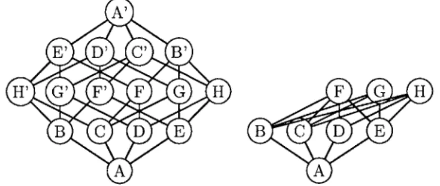
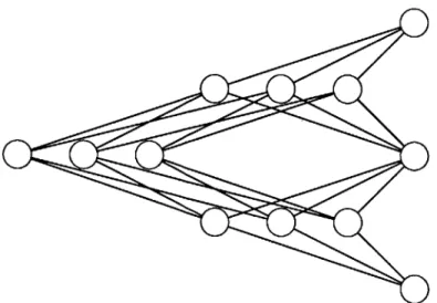
An (n, 0)-multichromotopoloy must be the n-cubical chromotopology, corre-sponding to the trivial code { 0 }. The smallest non-cubical adinkraizable chro-motopology, shown in Figure 2-1, is the quotient Ic/L for L = {O000,1111}, the

smallest non-trivial doubly-even code. Its underlying graph is the complete bipartite graph K4,4. A' E' D' C' B' H' G' F' F G H F G H B C D E B C D E A A

Figure 2-1: The graphs 14 and I4/{0000, 1111}. Labels with the same letter are sent to the same vertex.

While the problem of classifying adinkraizable chromotopologies reduces to that of classifying doubly-even linear codes, the theory of these codes is very rich and non-trivial. Computationally, [321 contains the current status of the classification through an exhaustive search. We invite the reader to explore the other connections between adinkras and coding theory (for example, the irreducible adinkraic representations correspond to the self-dual codes) from the original sources, such as

1121.

Finally, we remark that studying well-dashed chromotopologies is basically equiv-alent to studying Clifford algebras. Some of this intuition is suggested by the proof of Proposition 2.2.4. We discuss this further in Section 6.3.

Chapter 3

Dashings

Given a chromotopology A, define o(A) to be the set of odd dashings of A. Thus, adinkraizable chromotopologies are exactly those A with lo(A) > 0.

Problem 2. What are the enumerative and algebraic properties of o(A)?

In this section, we first generalize the concept of odd dashings to other graphs using the homological language we introduced in Section 3.1. We make some obser-vations of this generalized setting from other parts of mathematics, the closest link

being that of noneven graphs from the study of Pfaffian orientations.

Most of our results are on the enumeration of dashings of adinkraizable chromo-topologies, which is basically settled in this chapter. We introduce the concept of

even dashings and relate them to odd dashings, showing that not only do the even

dashings form a more convenient model for calculations, there is a bijection between the two types of dashings. We then count the number of (odd or even) dashings of

I, via a cute application of linear algebra and decompositions. Finally, we generalize

our formula to all chromotopologies with a homological algebra computation.

3.1

A Homological View

From the theorems in Chapter 2, we see that the n-cubical chromotopologies I, look like universal covers. We make this intuition rigorous in this section. We appeal to only basic techniques in homological algebra (any standard introduction, such as [24], is more than sufficient), but having another point of view greatly enriches the study of dashings on adinkras, as we will see in Section 3.5.

We work over Z2. Construct the following 2-dimensional complex X(A) from a

chromotopology A. Let CO be formal sums of elements of V(A) and C1 be formal sums of elements of E(A). For each 2-colored 4-cycle C of A, create a 2-cell with

C as its boundary as a generator in C2, the boundary maps {di: Ci -4 Cj_₁} are

the natural choices (we do not worry about orientations since we are using Z2),

giving homology groups Hi = Hi(X(A)). The most important observation about

Proposition 3.1.1. Let A be an (n, k)-adinkraizable chromotopology with L(A) = L. Then X(A) = X(In)/L as a quotient complex, where L acts freely on X(In). We have that X(Ig) is a simply-connected covering space of X(A), with L the group of deck transformations.

Proof. The fact that X(A) is a quotient complex is already evident from the

con-struction of the graph quotient, since we have restricted to simple graphs (recall that adinkraizable chromotopologies have simple graphs). It is easy to check that such an action is free for all i-dimensional cells if the codewords have minimal weight greater than i, and the minimal possible weight of our codes is 4.

A quick way to see that X(Ig) is simply connected is note that X(Ig) is the

2-skeleton of the n-dimensional (solid) Hamming cube Dn. Thus, X(In) and D must have matching H1 and r1, but D is obviously simply-connected. E

We have learned that there is some independent work by the original authors of the adinkras literature [101 using similar homological techniques. They work with the full complex and not just the 2-skeleton, which has some added benefits but also loses some properties we enjoy (for example, our L is free on the 2-skeleton for doubly-even codes L; this freeness is lost for higher-dimensional cells). We do, however, revisit their construction in Chapter 4 when we discuss Stiefel-Whitney classes of codes.

3.2

Generalizations and Sightings of Odd Dashings

In Section 3.1, we created a (cubical) complex X(A) from a chromotopology A by using A as the 1-skeleton and then attaching 2-cells for every 2-colored 4-cycle. One interpretation of this process is that we are distinguishing certain cycles (whose parities we care about when we dash A) and marking them via 2-cells.

Thus, an obvious generalization of odd dashings is the following: given a graph

G and a set of distinguished cycles C in G, call a dashing d: E(G) -+ Z2 an odd

dashing of (G, C) if for all cycles c E C, the sum of d(e) for e in c is odd. We then

call the set of odd dashings o(G, C). We can construct a 2-dimensional cell complex

X(G, C) by attaching 2-cells for every c E C. When G = In/L and C is the set of

2-colored 4-cycles in G, we recover our original definitions. Since we will always only have one C to consider at a time, we can suppress this notation and just write o(G)

instead of o(G, C) (and similarly for X(G)) once C is fixed.

The benefit of this generalization is that the odd dashings have a natural cohomo-logical interpretation: associate a dashing of (G, C) with an element of H1

(X(G, C), Z2)

in the natural way by sending each edge e to d(e). Then the distinguished element in H2

(X(G, C)) obtained by sending each 2-cell to 1 vanishes in cohomology if and

only if there is an odd dashing. This suggests that the homological approach may make some proofs easier, as we will exhibit in Section 3.5 (as all our calculations are done in homology, we do not directly use the cohomological observation we just made in this work. However, we would like to note that it plays a critical role in

Remark 3.2.1. We want to remark that not only do these generalized odd dashings

come up naturally in the study of adinkras, they have appeared elsewhere in math-ematics under different disguises. A frivolous example is that making the signs of a total differential consistent in a double complex requires changing signs in the grid graph of differential maps such that every square has an odd number of sign changes (see, for example, [5]). A more sophisticated example is in [2, Lemma 10.4], where the authors needed to exhibit an odd dashing on a poset structure of the Weyl group of a Lie algebra g in the construction of a g-module resolution. A uniform study of these occurrences would be very interesting.

3.3

Even Dashings

Let an even dashing be a way to dash E(G) such that every 2-colored 4-cycle contains an even number of dashed edges, and let e(G, C) (and again, just e(G) for short) be the set of even dashings. We have the following nice fact:

Lemma 3.3.1. If Jo(G,C) > 0, then we have Io(G,C) = Je(G,C).

Proof. Let 1 =

IE(G).

We may consider a dashing of G as a vector in Z1, where each coordinate corresponds to an edge and is assigned 1 for a dashed edge and 0 for a solid edge. There is an obvious way to add two dashings (i.e. addition in Z1) and there is a zero vector do (all edges solid), so the family of all dashings (with no restrictions) form a vector space Vfree(n) of dimension 1.

Observe that e(G) is a subspace of Vfre(n). To see this, we can directly check that adding two even dashings preserve the even parity of each 2-colored 4-cycle and that do is an even dashing. Alternatively, we can note the restriction of a dashing

d having a particular cycle with an even number of dashes just means the inner

product of d and some vector with four l's as support is zero, so such dashings are exactly the intersection of Vfr(n) and a set of hyperplanes, which is a subspace.

Unlike the even dashings e(G), the odd dashings o(G) do not form a vector space; in particular, they do not include do. However, adding an even dashing to an odd dashing gives an odd dashing and the difference between any two odd dashings gives an even dashing. Thus, o(A) is a coset in Vfrre(n) of e(G) and must then have the same cardinality as e(G) given that at least one odd dashing exists. E

Corollary 3.3.2. For any adinkraizable chromotopology A and C being the set of 2-colored 4-cycles, we have

Io(A,

C)I = Ie(A, C)|.

The proof of Lemma 3.3.1 hints that working with the even dashings may be slightly easier than the odd dashings, thanks to their vector space structure. Struc-turally, the intuition we gain is that the odd dashings form a torsor for the even dashings. Here is a linear algebraic explanation of these concepts that offers another (basically equivalent) proof of Lemma 3.3.1.

Consider the vector space V over Z2 indexed by the edges. We can then represent

to be the ICI x IE(G)

I

matrix where each row corresponds to a different cycle in C. Note we can represent a dashing by a column vector in ZIE(G). With this notation, even dashings are simply vectors that are annhilated by M(C) and odd dashings are vectors that map to the all l's vector. It is clear from this formulation that the cardinality of the latter set is either 0 (if the said vector has no preimage) or equal to the former set.

It is clear from this setup that our enumeration of even and odd (when they exist) dashings is equivalent to counting the dimension of the cycle space of cycles spanned

by C. We give this formulation in the following Proposition, though we will not use

it explicitly later.

Proposition 3.3.3. The number of even dashings, |e(G, C)|, is equal to 2r(M(C)),

where r(M) denotes the rank of M. The number of odd dashings, o(G, C)|, is either

0 or equal to e(G,C).

Proof. This is basically obvious from the proof of Lemma 3.3.1 and the observation

that r(M(C)) is exactly the dimension of the space of cycles generated by C. L

3.4

Decomposition and Dashings on Hamming Cubes

In this section, we resolve Problem 2 for Hamming cubes A = I,, with C being the

set of 2-colored 4-cubes. We will generalize the result later in Section 3.5, but we can gain some insights from this special case, the main observation being that dashings behave extremely well under a concept of decomposition.

Call a graph G decomposable if G = H x I, the cartesian product of some graph G and a single edge. Say that a color i decomposes a chromotopology A if removing

all edges of color i splits A into 2 separate connected components. In this case, we must have the underlying graph of A be decomposable. Our definition was inspired

by observations in [121, where certain adinkras were called 1-decomposable. As Greg

Landweber pointed out to us, the concept corresponding to decomposition in coding theory is punctured codes [271.

Lemma 3.4.1. The color i decomposes the chromotopology A if and only if for all

d E L(A), the i-th bit of d is 0.

Proof. This is a very straightforward verification. We leave the proof as an exercise

to the reader.

Corollary 3.4.2. Every color in [n] decomposes In.

In the situation where Lemma 3.4.1 holds, we say that i decomposes A into A0

and A1, or A = A0 II A1, if removing all edges with color i creates two disjoint

chromotopologies A0 and A1, which are labeled and colored in a natural fashion,

* V(A) can be partitioned into two

V(A10) have 0 in the i-th bit (by

and vertices in V(All) have 1 in

V(AO) and V(Al1) are of color i.

sets V(AO) and V(All), where vertices in

Lemma 3.4.1, this is a well-defined notion)

the i-th bit. Furthermore, all edges between

" define AO to be isomorphic to the edge-colored graph induced by vertices in

V(A 0), where any codeword v

=

(blb

2

... b,) in the vertex label class of V'

E

V(AO) is sent to the (n -

1)-codeword

(bib2 ... bi ... bn), where we remove the

bit bi. Color the edges analogously with colors in {1, 2--- ,i,-

,

n}. Define

A

1 in the same way with V(All) instead of V(AO).

" define the maps inc(bib2 ... b- 1,7j -+ i) = b₁ ... b.. ₁jb₁ ... b.- ₁, which inserts

j into the i-th place of an (n - 1)-codeword to create an n-codeword. If A =

AO

1I2 A

1

,

let inc(v) send a vertex v E Aj to inc(v,j -+ i) for j E {0, 1}.

Lemma 3.4.1 gives that the union of the image of V(Ao) and V(A1) under inc

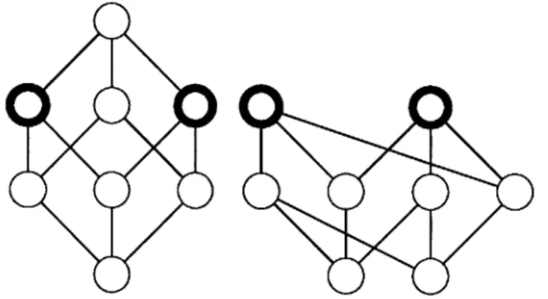
is exactly V(A). 111 011 101 110 001 010 100 000

~11

01 10 11 00 0110 00

Figure 3-1: The color 3 decomposes a ranked chromotopology A (with chromotopology

I3)

as

A

= A0113

A

1. Each

Ai

has chromotopology

I2.

Proposition 3.4.3. Let A

=

AO Hi A

1

, where A is an (n, k)-chromotopology.

Ao and A

1

are (n

-

1, k) chromotopologies, isomorphic as graphs.

Then

Proof. The image of qj on V(Ao is exactly V(A

1

) and qj is an involution, so we

have a bijection between the vertices. If qj(vi)

= V2

in A

0

, the 4-cycle condition

on

(V

1

, qj(v

1

),

qi(v2), v2) gives that (qi(vl),q(v2)) is also an edge of color

j

in

A

1

,

so the bijection between the vertices extends to a bijection between AO and A

1

as

edge-colored graphs, and thus chromotopologies. Each of these chromotopologies has

2-1 vertices and is (n - 1)-regular, so by Proposition 2.1.1 they must be (n - 1,

We now prove our main idea, which tells us that dashings of decomposable graphs are easy to compute recursively.

Lemma 3.4.4. If A has 1 edges colored i and A = AO IIj A1, then each even (resp. odd) dashing of the induced graph of AO and each of the 21 choices of dashing the i-colored edges extends to exactly one even (resp. odd) dashing of A.

Proof. Without loss of generality, we can take i = 1, so AO contains equivalence

classes of codewords with first bit 0 and A1 contains those with first bit 1.

After an even dashing of AO and an arbitrary dashing of the i-colored edges, note the remaining 2-colored 4-cycles are of exactly two types:

1. the 4-cycles in A1;

2. the 4-cycles of the form (u, v, W, x), where (u, v) is in AO, (w, x) is in A1, and

(v, w) and (x, u) are colored i.

Note that in all the cycles (u, v, w, x) of the second type, (w, x) is the only one we have not selected. Thus, there is exactly one choice for each of those edges to satisfy the even parity condition. Since there is exactly one such cycle for every edge in

A1, this selects a dashing for all the remaining edges, and the only thing we have to

check is that the 4-cycles of the first type, the ones entirely in A1, are evenly dashed.

Now, a 4-cycle of this type is of form (1l, 1a2, 1 3, 1a4), which is a face of a

3-cube with vertices (Ga1, Ga2, Ga3, Ga4, 1a1, 1a2, 1a3, 1a4). There are 5 other 4-cycles

in this Hamming cube which have all been evenly dashed (the Gaj vertices form a cycle in AO and the other 4 cycles are evenly dashed by our previous paragraph). Thus, we have that:

d(Gai, Ga2) + d(Ga2, Ga3) + d(0a3, Ga4) + d(Oa4, Ga1) = 0;

d(Gai, Ga2) + d(Ga2, 1a2) + d(la2, la) + d(lai, Gai) = 0;

d(0a2, Ga3)

+

d(Ga3, 1a3)

+

d(la3, 1a2)

+

d(la2, Ga2) = 0;

d(0a3, Ga4)

+

d(0a4, 1a4)

+

d(la4, 1a3)

+

d(la3, Ga3) = 0; d(Ga4, Ga1) + d(Gai, la) + d(lai, 1a4) + d(la4, Ga4) = 0.

Adding these equations in Z2 gives:

d(lai, 1a2) + d(la2, 1a3) + d(la3, 1a4) + d(la4, 1a1) = 0.

Thus, we have constructed an even dashing. The analogous result for odd dashings follow if we replace O's on the right sides of the above equations by l's. L

Remark 3.4.5. This proof is easily seen to generalize to dashings of (A x I, C),

where the cycles of C occur in a "mirrored" fashion in the two halves of the graph, and all 4-cycles that use the edges corresponding to I belong to C.

Proposition 3.4.6. The number of even (or odd) dashings of In is

e(I)| = o(In)| = 22-1

Proof. A convenient property of Hamming cubes is that every 4-cycle is a 2-colored

4-cycle. Thus, we get to just say "4-cycles" instead of "2-colored 4-cycles" in this proof.

We prove our result by induction. The base case is easy: for n = 1 (a single edge), there are exactly 2 even dashings, since there is no 4-cycle. Suppose our result were true for every k < n. We will now show it is also true for n. Recall from Corollary 3.4.2 that every color decomposes In into two smaller Ic"'s. Since we have 2n-1 edges with color 1, by Lemma 3.4.4 we get the recurrence

le(I ) = 2n- eI22Th

,

I-With the initial case e(Ic)= 2, we get Ie(I"n)I = 22n-h +2-2+..-+1 = 22n-1, as desired. The result for Io(I")| is immediate by Lemma 3.3.1. L

Note that Io(Ic") = 22/2. This suggests that, besides a single factor of 2, each of the 2"n vertices gives exactly one "degree of freedom" for odd dashings. We will justify this hunch in the following discussion, in particular with Proposition 3.5.1.

3.5

Dashings on Adinkras

In this section, we generalize Proposition 3.4.6 to all adinkraizable chromotopologies, where A is some adinkraizable chromotopology In"/L and C is again the set of 2-colored 4-cycles. We will use the idea of vertex switching and some homological algebra.

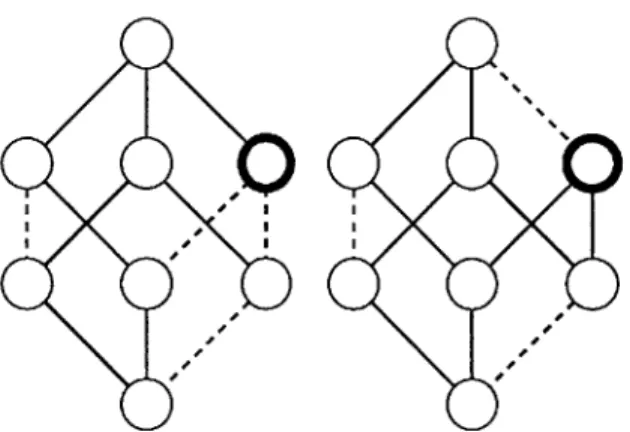
In [131, Douglas, Gates, and Wang examined dashings from a point of view in-spired by Seidel's two-graphs ([361). Define the vertex switch at a vertex v of a well-dashed chromotopology A as the operation that produces the same A, except with all edges adjacent to v flipped in parity (sending dashed edges to solid edges, and vice-versa). It is routine to verify that a vertex switch preserves odd dashings (in fact, parity in all 4-cycles), so the odd dashings of A can be split into orbits under all possible vertex switchings, which we will call the labeled switching classes

(or LSCs) of A. We emphasize the adjective "labeled" because the term switching class in [13] refers to equivalence classes not only under vertex switchings, but also

under different types of vertex permutations.

In the representation theory interpretation of adinkras (see Section 1.4), a vertex switch corresponds to adding a negative sign in front of a component field, which gives an isomorphic representation. Thus, it is natural to think about equivalence classes under these transformations. The following computation will not only be useful to study switchings, but will also justify our hunch about the "degrees of freedom" from Proposition 3.4.6.

Figure 3-2: Before and after a vertex switch at the outlined vertex.

Proposition 3.5.1. In an adinkraizable (n, k)-chromotopology A, there are exactly 22n-k-1 dashings in each LSC.

Proof. Vertex switches commute and each vertex switch is an order-2 operation, so

they form a Z2-vector space, which we may index by subsets of the vertices. Consider

a set of vertex switches that fix a dashing. Then, each edge must have its two vertices both switched or both non-switched. This decision can only be made consistently over all vertices if all vertices are switched or all vertices are non-switched. Thus, the 2n-k sets of vertex switches generate a Z2-vector space of dimension 2n-k - 1.

This proves the result. E

Corollary 3.5.2. The cubical chromotopology In' has exactly one labeled switching class.

Proof. This is immediate from Proposition 3.5.1 and Proposition 3.4.6, with the

substitution k = 0. Alternatively, this is also evident from [13, Lemma 4.1]. L

Finally, we combine several ideas (even dashings, vertex switchings, and our cell complex interpretation of chromotopologies) to generalize Proposition 3.4.6.

Proposition 3.5.3. Let A be an adinkraizable (n, k)-chromotopology. Then there are 2k LSCs in A.

Proof. First, vertex switchings preserve parity of all 4-cycles, so counting orbits of

odd dashings (LSCs) under vertex switchings is equivalent to counting orbits of even dashings.

An even dashing can also be thought of as a formal sum of edges over Z2 (we

dash an edge if the coefficient is 1 and do not otherwise), which is precisely a 1-chain of X(A) over Z2. Second, the even dashings are defined as dashings where all

boundaries of C2, the even dashings are exactly the orthogonal complement of Im(d2)

inside of C1 by the usual inner product. Thus, the even dashings have Z2-dimension:

dim((Im(d₂)') = dim(C1) - dim(Im(d2))

= (dim(ker(di)) + dim(Im(di))) - dim(Im(d2))

= dim(H1) + dim(Im(di))

= dim(H1) + dim(Co) - dim(Ho).

However, note that dim(Co) - dim(Ho) = 2n-k - 1, which is exactly the dimen-sion of the vector space of the vertex switchings for a particular LSC from Propo-sition 3.5.1. Since the product of the number of LSCs and the number of vertex switchings per LSC is the total number of even dashings, dividing the number of even dashings by 22 -- 1 gives that the dimension of switching classes is precisely

dim(H1).

By Proposition 3.1.1 and basic properties of universal covers and fundamental

groups, ri(X(A)) = L, the quotient group, which in this case is the vector space

Z2. Also, H1 = Z2 since H1 is the abelianization of 7r. Thus, we have 2k switching

classes. L

Propositions 3.5.3 and 3.5.1 immediately give:

Theorem 3.5.4. The number of even (or odd) dashings of an adinkraizable (n,

k)-chromotopology A is

|e(A)|I =

o(A)I

= 2 2-k+k-1

A surprising but neat consequence of this result is that the number of dashings

does not depend on the actual code L(A), rather just on its dimension. This is very nonintuitive to see with elementary combinatorial methods. In either case, this sec-tion shows that the dashing enumerasec-tion problem on adinkras is mostly understood.

3.6

A Generalization of Dashings and Noneven Graphs

We started out with a notion of odd dashings for adinkras. In Section 3.2 we gener-alized this notion to odd (and even) dashings on general undirected graphs.

The concept of noneven graphs from the theory of Pfaffian orientations (for a reference, see [39]) is similar to odd dashings, but are defined for directed graphs instead of undirected graphs. In this section, we develop a generalization of noneven graphs and odd dashings on adinkras. The reader should take care to note that this

is an independent direction of generalization as the generalization in Section 3.2. For an undirected graph G and a set of even-lengthed cycles CG, let an (edge)

orientation of G be a directed graph with the underlying undirected graph G. Now,

define an odd orientation (relative to CG) to be an orientation of G where each cycle in CG has an odd number of edges oriented in either direction (equivalently, both