HAL Id: hal-02152147
https://hal.archives-ouvertes.fr/hal-02152147
Submitted on 11 Jun 2019HAL is a multi-disciplinary open access archive for the deposit and dissemination of sci-entific research documents, whether they are pub-lished or not. The documents may come from teaching and research institutions in France or abroad, or from public or private research centers.
L’archive ouverte pluridisciplinaire HAL, est destinée au dépôt et à la diffusion de documents scientifiques de niveau recherche, publiés ou non, émanant des établissements d’enseignement et de recherche français ou étrangers, des laboratoires publics ou privés.
Modified Finite Volumes Method for the Simulation of
Dynamic District Heating Networks
Manuel Betancourt Schwarz, Mohamed Mabrouk, Carlos Santos Silva,
Pierrick Haurant, Bruno Lacarrière
To cite this version:
Manuel Betancourt Schwarz, Mohamed Mabrouk, Carlos Santos Silva, Pierrick Haurant, Bruno Lacar-rière. Modified Finite Volumes Method for the Simulation of Dynamic District Heating Networks. Energy, Elsevier, In press, 182, pp.954-964. �10.1016/j.energy.2019.06.038�. �hal-02152147�
Modified Finite Volumes Method for the Simulation of
Dynamic District Heating Networks
Manuel Betancourt Schwarza, Mohamed Tahar Mabroukb, Carlos Santos Silvac, Pierrick Haurantd,Bruno Lacarrièree
a IMT Atlantique – IST de Lisboa, 4 rue Alfred Kastler, 44307 Nantes cedex 3, France,
b IMT Atlantique, UMR CNRS GEPEA, 4 rue Alfred Kastler, 44307 Nantes cedex 3, France,
c IST de Lisboa, Universidade de Lisboa, Av. Rovisco Pais 1, 1049-001 Lisboa, Portugal,
d IMT Atlantique, UMR CNRS GEPEA, 4 rue Alfred Kastler, 44307 Nantes cedex 3, France,
e IMT Atlantique, UMR CNRS GEPEA, 4 rue Alfred Kastler, 44307 Nantes cedex 3, France,
Abstract:
District Heating (DH) networks are getting closer to the concept of “Smart Grids” to deal with the contribution of new technologies and paradigms like Renewable Energy Sources, Distributed Generation and Storage, and Low-Temperature District Heating. This requires good anticipation of the system’s dynamics with the objective of improving control. This work proposes a model based on the Finite Volumes method for anticipating the dynamics in DH systems. Its application to branched network topologies gives the delay between the change in the settings at the generation points and the time they are perceived by the different substation in the network, which is a prerequisite for system design, operation planning and optimal control. The model is tested in a 6 Node branched network with the main topology elements being represented (junctions, splits, etc.); real demand data is used at the consumption nodes. A comparison between the model developed by the authors and the existing Finite Volumes method is also presented for the proposed topology. These results shed light on the needs and opportunities in DH, mainly for ICT implementation, energy storage location and management, and enhanced control in the smart energy networks context.
Keywords:
District Heating, Smart Thermal Networks, Transient Modeling. Finite Volumes
1. Introduction
District Heating (DH) is a system that supplies heat to different users connected to centralized or distributed heat generation units through a network of pipes. The scale of these systems varies from building facilities to a complete city. The management of DH networks has long been considered to be a static problem since operative control is kept to a minimum and the network is reconfigured only occasionally [1–3]. This model of design and operation is proving to be outdated [4]. The increasing use of Renewable Energy Sources, Distributed Generation, Low Energy Buildings, Distributed Storage and the possibility of developing Low-Temperature District Heating, among others, is demanding a change in the way DH is planned and operated. This change could come in the way of Smart Thermal Networks [4–6].
Smart Networks (SN) is a relatively new concept that gained international attention when the electricity sector started to apply them in what we now call Smart Grids [7]. Most authors [8–11] agree that SN are systems capable of: 1) making automated decisions concerning the current and future status of the network to guarantee its expected operation and 2) integrating all users
connected to it and enabling them to participate actively in the activities of the network. The overall objective is that the grids have higher efficiencies (economic and technical) and sustainability while maintaining the Quality of Service (QoS).
In the future, District Heating is expected to connect low energy buildings through low-temperature networks with increased efficiency where renewable energies and distributed generation are smoothly integrated [12]. These systems will be economically and environmentally sustainable. To do so, DH will rely heavily on Communication and Control infrastructures. In analogy with Electric Smart-Grids, Smart Thermal Networks will depend on Information and Communication Technologies (ICTs) for quality monitoring, timely information exchange and effective control [13].
Currently, the level of monitoring and measurement in DH is very low and instrumenting existing networks can be very costly. Nevertheless, future networks are expected to have a higher level of metering and monitoring, for this reason a different way of assessing the impact of technological and operational changes has been pursued in the form of Modeling and Simulation (M&S) [14–17]. With M&S it is possible to replicate existing DH systems and modify them virtually to evaluate the possible results without incurring in high costs.
In the literature two main approaches have been pursued for the modeling of DH, the black box models and the physical models[2]. The former are data-driven models that consider only the input and outputs of the system and are known for their speed but low accuracy on highly dynamic systems. The latter are based on the physical aspects of the system and are preferred for modeling when there are high or quick variations of the temperature or when information from within the pipes is relevant.
Many examples exist in the literature of physical models and they can be classified according to their different approach. Some of the first methods were the element method, the characteristic method and the node method. Both the element method and the characteristic method rely on discretizing the pipe into a finite number of elements and then computing each element individually by treating the flow of water as an advection-diffusion equation, where the output of one becomes the input of the next as to follow the temperature propagation. As early as 1979, [18] presented the QUICK scheme for solving the heat transport equation using the element method.
In the case of the node method, the outlet temperature is calculated based on the inlet temperature and the delay of the propagation. Both the element method and the node method are described in [19] and later were compared in [20] showing better and faster results for the node method. This method was used in [21,22] to model the Naestved DH system in Denmark. The model’s results are compared with the commercial software TERMIS and show that for near-steady state conditions the difference is negligible but the studied model has issues with sudden or large changes in the temperature and with long pipelines.
Similar to the element method, the characteristic method discretizes the pipe but the equations for heat transport are transformed into an ordinary differential equation along the characteristic lines so a solution can be obtained. In [23] the authors propose a hybrid method where the momentum equation is solved using the SIMPLE scheme approach and the energy equation is solved with the method of characteristics in combination with Lagrange polynomial interpolation. The method is used to predict the propagation of the enthalpy front and locations where a boiling boundary condition during the transient of the flow could occur with good results. A model based on the characteristic method was used in [24] to model the district heating system in Zemum, Serbia. In this work the thermal transient of a system is analyzed and the results compared with measured data; results show good matching between the two with no significant numerical diffusion. Another methodology based on this was later developed by [25] and validated with the DH network in the city of Linyi, China. The model was able to reproduce the behavior of the network with an error below 4% for the farthest nodes. A modified approach of the characteristic method is presented in [26], where the authors use a model based on the method of characteristics while considering the difference between the turbulent flow and the boundary layer. This approach shows low
computational times and good accuracy at different values of Reynolds numbers; the model is further validated by data gathered from real pipes.
Other methods have been proposed that have gains in speed, accuracy or level of detail. The Function Method, presented in [2], considers the mass flow rate, the losses and the inertia and obtains the analytical solution to the transient energy equation by using the expansion of Fourier series. This method proves to be 37% faster than the Node Method while being more accurate during rapid changes in the temperature. A method to optimize the parameters used by the Function Method is proposed in [27], where the authors use measured data to find the equivalent pipe length that better approximates the output temperature of the pipes. A method using the polynomial approximation for the steady state model of a DH network is presented in [28] to find strategies to operate DH when there is uncertain or variable demand. The authors use this model to minimize the cost of generation in a DH network under different operation strategies. Finally, a modeling approach based on the Finite Volumes method is presented in [29]. The method, named the implicit upwind method, is compared to the characteristic line method and the authors conclude that the characteristic line is faster but the implicit upwind method provides more information on the temperature distribution within the pipe.
In [30] the authors present a model based on the standard TRNSYS Type 31 component, which is based on the Lagrangian approach. The model, named the plug flow model, is compared to a 1D and a 2D Finite Volumes model. The results show that the plug flow gives the same accuracy as the 1D model while using a rougher spatial discretization and presents more robustness for very long pipes. The need of fewer elements in the discretization also allows the plug flow model to be run much faster than the 1D model. This approach is later used by [31] to model district cooling networks where the results show it to be reliable for its implementation during the design phase or the optimization of the operation. Another model based on plug flow was developed by [32]. The model was implemented in Modelica, compiled and simulated in Dymola and made use of the Dassl solver. The results showed good correspondence when compared to a multiple control volume model, with faster computing time and better response in faster dynamics.
This paper introduces a new modeling approach that combines the finite volumes method (FVN) with the electric analogy of heat transfer to compute the losses and inertia in the grid with greater robustness for variable flows. The combination of FVN with the electrical analogy allows reducing the numerical diffusion in long pipes while keeping the computational times relatively low. In the next section the physical and mathematical basis is explained and the emphasis is made on how the model is capable of performing more accurately than the existing FVN during dynamic operation.
2. Methodology
DH can be represented as a network of interconnected nodes [20], where generation and consumption sites are the nodes, and the vertices/edges connecting them are the buried-underground supply and return pipes transporting the water. For this reason, the model developed in this work is composed of two sub-models, one representing the pipes and another one the generation and consumption nodes. The response to the change of the inputs or outputs is expressed as a spatial-temporal distribution of temperatures and mass flow rates in the system.
The sub-model representing the pipes, namely the Heat Transport sub-model, is modeled on the physical phenomena of Mass Transport and Heat Transfer in a pipe and is based on the existing FVN. In FVN the pipes are discretized in smaller elements and an energy balance is done for each of them at every time step. The radial flows are unique to each element but they are connected through the axial flows, where the inputs for each element are the outputs from the previous one and the outputs become the inputs of the next element. In the Modified method the axial component of the FVN is kept but the radial flows are now calculated using the electrical analogy for thermal systems by modeling the system as an RC circuit. A comparison between this Modified method and the FVN method will be presented.
The sub-model representing the network, namely the Distribution sub-model, uses oriented graphs in combination with energy and mass conservation equations, head loss calculation and time series to compute the processes happening in every node. At every node an enthalpy and mass balance is performed to calculate the energy generated, consumed and passed on to the rest of the network as well as the temperatures in the supply and return sides. Both sub-models used together evaluate the direction, attenuation, delay and damping of the heat train across the network in the supply line and the return pipes.
Considering that the pressure wave propagates about 1000 times faster than the temperature wave, the flow occurs under low velocity conditions and the fluid used in Heat Networks is liquid water the following assumptions are made without significant loss of precision [24,25,27]:
▪ the flow is one-dimensional and incompressible; ▪ the effects of hydraulic dispersion are neglected; ▪ thermal diffusion, and axial heat transfer are neglected; ▪ heat dissipation is ignored due to low velocity flows;
▪ the specific heat at constant pressure ( ) is constant in the evaluated range;
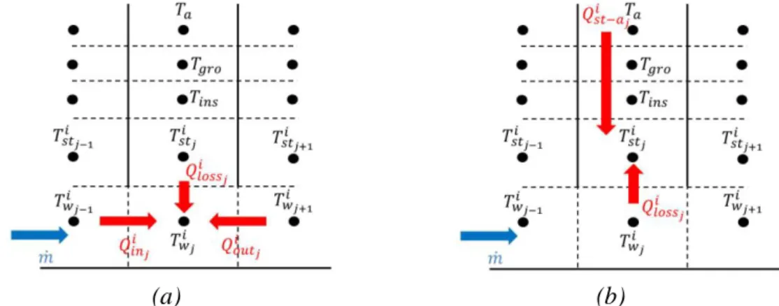
▪ each element of the discretized pipe has a lumped mass with a single temperature (no stratification inside the element, see Fig. 1);
▪ heat inertia of insulation and ground are ignored.
These considerations are similar to those taken in other works which report accurate results for the modeling of thermal networks [14,24,26,30,32]. Both models are further explained in the following sections.
(a) (b)
Fig. 1: a) Enthalpy balance for the water in element j of the pipe. b) Enthalpy balance for the steel in element j of the pipe. T are the temperatures; is the mass flow rate of the water; and Q are the heat flows.
2.1. Heat Transport sub-model
The Heat Transport sub-model derives from the enthalpy balance for the energy flows in a discretized pipe. The energy flow, or heat flow, is composed by the axial component, which is the heat carried by the water along the pipe, and the radial component, which is the heat that the water loses through the walls of the pipe. The enthalpy balance is written for every pipe element, each has three associated heat flows that determine the change in its stored energy ( ). On the axial axis
we have the heat that flows in from the upstream element ( ) and the heat that is passed to the downstream element ( ). On the radial axis there is the heat that is lost through heat transfer during the time the water is in the evaluated element ( ). This heat depends on the difference in temperatures between the pipe wall and the water. The enthalpy balance for an element of the pipe at time is shown in Eq. (1).
The balance in Eq. (1) can be expressed using the two variables for the system: the mass flow rate ( ) and the temperature ( ) of the water. In explicit form, these can be seen in Eq. (2a-2d).
2.1.1 FVN method
To solve the enthalpy balance it is necessary to know the temperature of the steel ( ) in order to calculate the losses. In the FVN method a second enthalpy balance is made for the steel pipe as shown in Eq. (3). In this case the change of the energy in the steel pipe is caused by the heat transferred from the water to the pipe ( ) and the heat transferred from the pipe to the environment ( ). The former is indicated on the item at the right side of the equality in Eq. (3) and the latter on the item at the left of this equality. In this equation is the ambient temperature and is the resistance between the steel pipe and the surroundings (including insulation resistance and soil resistance).
(3)
Equations (1) and (3) define the matrix system shown in (4) .
(4) 2.1.2 Modified method
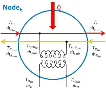
In the Modified method is obtained using the electrical analogy of the system. The thermal
conductivities are associated to electrical resistances, the heat capacities to electrical capacitances and the temperature gradients to voltage difference. The system can be solved as an RC circuit [33]. The converted circuit for a pipe like the one shown in Fig. 1 is shown in Fig. 2:
Fig.2: Thermal Circuit for an insulated pipe considering only one capacitance.
In Fig. 2, is the temperature of the water, is the temperature at the middle of the steel pipe,
is the temperature of the insulation, is temperature of the soil and is the ambient
temperature. is the thermal resistance of the water (obtained from the convective heat transfer
coefficient of the water and the area of contact between water and steel) and half the thermal resistance of the steel pipe; is the resistance of the other half of the pipe, the insulation and the soil. is the heat capacitance of the steel pipe and is equal to: [34]. is
calculated using the resistance equivalent for a cylindrical geometry and the shape factor for a constant temperature cylinder buried in a half infinite domain [33].
(2a) (2b)
(2c)
The solution for the circuit in Fig. 2 for the change from time step to time step can be found using the Laplace transform of the system [35]. Using as the reference temperature for this
change the resulting system of equations can be seen in Eq. (5).
(5)
is the time constant of the system and is defined by Eq. (6).
(6)
By solving the system of equations shown in Eq. (5) it is possible to solve the enthalpy balance for any pipe element .
2.2. Distribution sub-model
The modeling of branched DH networks is done through the use of oriented graphs. Every vertex/edge of the graph corresponds to a pipe with the associated characteristics pertaining to it (length, diameter, material, insulation, etc.). Every node of the oriented graph corresponds to a node of the network (i.e. substations, junctions or splits) and it contains the information regarding to local generation, consumption or storage in the form of equations or time series. The graph transforms the physical connection of the network into a matrix called the Adjacency Matrix [36].
The characteristics associated to the edges are uploaded from a database of various DH pipes. Then the pressure needed at the output of the node to maintain the mass flow is calculated using the Darcy-Weissbach equation for head loss in the pipe Eq. (7).
(7)
In this equation is the length of the pipe, is the speed of the flow, is the gravity, is the diameter of the pipe and is the friction factor. This last parameter can be calculated using Eq. (8), an explicit equation introduced by Barr [37], which provides accurate results for Reynolds numbers higher than . In Eq. (8) is the effective roughness and Re is the Reynolds’ number.
(8)
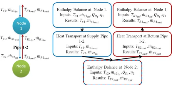
The next step is to model the processes at the different nodes. To exemplify the enthalpy balance in a node Fig. 3 shows a substation node with a local heat source. In this figure we can see that a node with local generation has 5 mass flow rates ( ) and 6 temperatures ( ) that have to be determined (other nodes may have a
different balance, i.e. a node with no local heat generation and no consumption has 2 temperatures):
1. Two supply temperatures ( ) and two mass flow rates ( ) at the supply line.
2. Two return temperatures ( ) and two mass flow rates ( ) at the return line.
Fig. 3: Representation of a Node and its flows in a DH system.
The temperatures and mass flow at the secondary side of the heat exchanger ( ) are not in the scope of this paper and are not further analyzed.
The input mass flow rates and temperatures for the supply and return lines depend on their upstream nodes. The temperature and mass flow rates at the heat exchanger of the substation can be obtained once the demand ( ) and the heat exchangers efficiency ( ) are known (calculating the heat exchangers efficiency is outside the scope of this work, so it is assumed to be known). The output mass flow rates and temperatures of the supply and return lines can be calculated once their input temperatures and mass flows and the mass flow of the heat exchanger are known
It is possible to see that most of the data needed for the balance at the nodes is obtained from the Distribution Model. The only values that are not obtained from this model are and . And to obtain these values it is necessary to couple the Heat Transport model and the Distribution sub-model together.
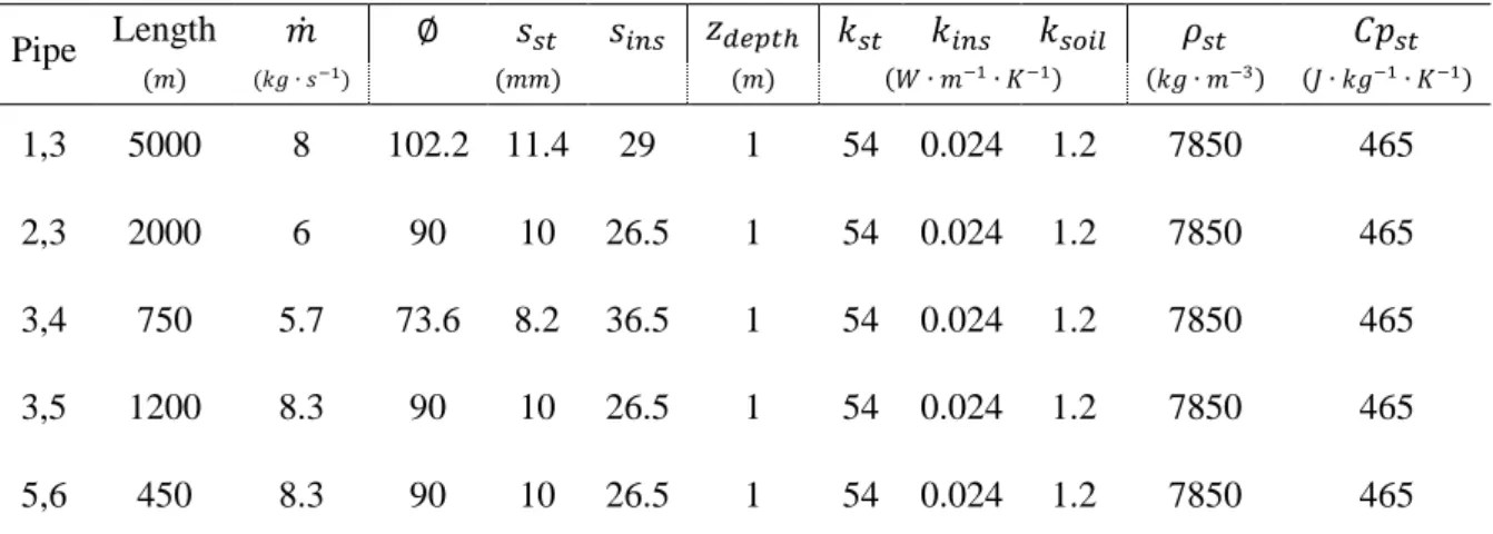
2.3. The coupled model
The Fig. 4 shows how two sub-models are combined together to represent the DH network. The Distribution sub-model recreates the topology and the node dynamics (generation, consumption, storage) and the Heat Transport sub-model simulates the transport phenomena and the heat losses. In this example two nodes are analyzed with Node 2 being an end of the line node (any mass flow not consumed by the substation is injected directly into the return line). The temperatures and mass flow rates are calculated for every time step . The resulting supply temperatures and mass flow rates from Node 1 are fed into the supply Pipe 1-2 towards Node 2. Because Node 2 is at the end of the line, its results are fed to the return Pipe 1-2, which in turn are fed into Node 1. This process is repeated for any number of nodes, always starting from the first upstream nodes to the end of the lines for the supply line and from the last downstream nodes to the first upstream nodes for the return line. In addition, the Distribution sub-model considers the existence of junctions and splits and calculates the respective enthalpy and mass flows of each branch accordingly.
Fig 4: Diagram of the coupled model for two nodes. Node 2 is an end of the line node.
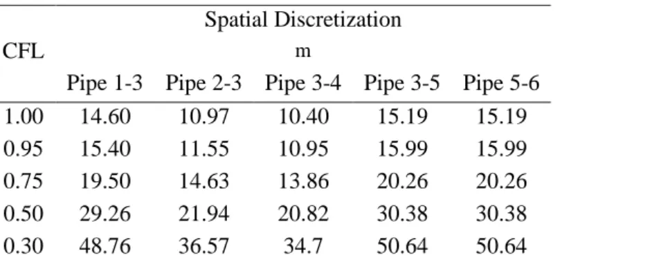
As the proposed model is based on the Finite Volumes method, the spatial and temporal discretization is very important to guarantee stability and prevent numerical diffusion. To ensure the reliability of the results, the volume of the water evaluated in one element has to be equal or greater than the volume of the flow of water entering the element. This constraint is known as the Courant-Friedrich-Levy condition ( ). If the system presents numerical instability; if the system presents numerical diffusion.
In our Modified method the temporal discretization is fixed during the whole simulation and can be set to any desired value. The spatial discretization is then calculated using the temporal discretization, the target CFL and the maximum expected flow rate for each pipe during the simulated period. In this way, every pipe has their own spatial discretization depending on their length and expected flow while keeping the temporal discretization constant. In cases when the mass flow does not vary this will guarantee the target CFL as well.
Nevertheless, constant mass flow rates are not usually the case in real networks. Substations in a real network can be set to allow a constant flow, but this operation strategy may not meet the QoS. Often the mass flow consumed at each substation will depend on the supply temperature and the demand. Because
is fixed in our simulations, and always meeting the demand is a
constraint, the energy extracted at each substation will vary at different time steps. This will cause the network to present variable mass flow rates in the outlet of the nodes ( ), even if the mass flow rate at their inlet is constant ( ).
Trying to keep the CFL=1 at every time step can be very computational intensive. Instead of recalculating the spatial discretization constantly, the Modified method keeps it constant for a range of CFL values, only recalculating if the CFL is out of this range ( ). Doing this allows for accurate results for a higher range of CFL without increasing the computational times.
3. Case Study
Two case studies are presented in this paper. In the first case study a simple network composed of 6 Nodes and 5 Pipes is analyzed (Fig. 5). The network contains two generation nodes (Nodes 1 and 2) and 4 consumer nodes (Nodes 3 – 6). The pipes’ length and properties are described in Table 1. The network is simulated for the pre-heating process, where the temperature of the network is raised while no demand exists (e.g. early in the morning to anticipate the peak demand). This case study is evaluated using the FVN and the Modified method which are compared. For the second case study the same network will be simulated using the Modified method, but this time during the normal operation of the District Heating network using heat demand data based on the real measurement analysis from a network in the city of Nantes, France.
Fig 5: Oriented Graph for the 6 node branched network used for the case study simulations. Pipe Length 1,3 5000 8 102.2 11.4 29 1 54 0.024 1.2 7850 465 2,3 2000 6 90 10 26.5 1 54 0.024 1.2 7850 465 3,4 750 5.7 73.6 8.2 36.5 1 54 0.024 1.2 7850 465 3,5 1200 8.3 90 10 26.5 1 54 0.024 1.2 7850 465 5,6 450 8.3 90 10 26.5 1 54 0.024 1.2 7850 465
Table 1. Characteristics of the Pipes used in the Network Simulation.
In both case studies, the generation plants at Node 1 and 2 operate at a constant temperature while the consumption nodes are not supplied until their temperature reaches the minimum supply temperature. The mass flows in Table 1 are the initial flows for the simulation.
4. Results
The results for the two case studies are presented in this section. For the first case the results show the comparison between the FVN method and the Modified method. The results from both methods are compared for different CFL values.
The results for the six-node network using the Modified method illustrate the relevance of the modeling tool and its accuracy in representing the dynamic of heat and mass transfers in a realistic DH system.
4.1. Comparison between FVN and Modified method
The results for the first case study are presented in this section. The network was simulated for a period of 5 hours with a 15s time step using the FVN and the Modified methods. Every method is simulated for 5 CFL values: 1, 0.95, 0.75, 0.5 and 0.3. The ambient temperature is kept constant at 20°C for the duration of the simulation.
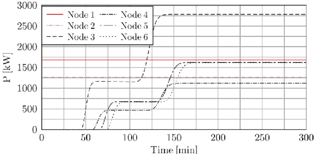
Fig. 6 shows the results for all nodes in the network for both modeling methods using a CFL=1. The FVN method took 724s to simulate and the Modified method took 763s to run. The spatial discretization can be found in Table A-1 in the Annex. In Fig. 6 it can be seen that both methods perform similarly. It can also be seen that for this network, the delay between generation and consumers varies between 135 min and 170 min. The stepped profile of the temperature in Fig. 6 is due to the distance of each generation plant, as the heat train from Node 2 arrives over one hour before the heat train from Node 1.
Fig. 6: Available Power Comparison at every node in the network for the FVN method (solid line) and the Modified method (marker) with CFL=1.
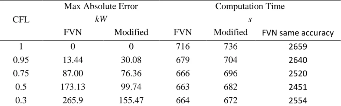
After confirming that both methods give the same results for CFL=1, a comparison for the results using different spatial discretizations (different CFLs) was performed. The results for the nearest node (Node 3) and farthest node (Node 6) using FVN are shown in Fig. 7 and on Fig. 8 for the Modified method. In these two figures it can be observed that the modified method presents less numerical diffusion as the spatial discretization increases (lower CFL). To better visualize these results, under each Power graph the absolute error can be found for all 4 cases using CFL=1 as reference. These graphs show that for the FVN method the maximum error varies between 13.44kW for CFL=0.95 and 265.9kW for CFL=0.3. For the Modified method the error varies between 30kW for CFL=0.95 and 155.47kW for CFL=0.3. The maximum absolute error as well as the computation times for the different CFL values can be seen in Table 2. The time needed to obtain similar error with the FVN method is also presented in this Table.
a) b)
Fig. 7: a) Power Available and Absolute Error at Node 3 for 5 CFL values using the FVN method; b) Power Available and Absolute Error at Node 6 for 5 CFL values using the FVN method.
a) b)
Fig. 8: a) Power Available and Absolute Error at Node 3 for 5 CFL values using the Modified method; b) Power Available and Absolute Error at Node 6 for 5 CFL values using the Modified method.
CFL
Max Absolute Error kW
Computation Time s
FVN Modified FVN Modified FVN same accuracy
1 0 0 716 736 2659
0.95 13.44 30.08 679 704 2640
0.75 87.00 76.36 666 696 2520
0.5 173.13 99.74 663 682 2451
0.3 265.9 155.47 664 672 2554
Table 2: Max Absolute and Relative Errors for different CFLs using FVN and the Modified method. These results show that the Modified method has better robustness than the FVN method for smaller CFL values, although the FVN method has better accuracy for CFL values closer to 1. As in a dynamic system the CFL can vary greatly during time, the robustness of the modified method is preferred when the system presents continuous changes in temperature and mass flow rates. In Table 2 it can be seen that to obtain the same absolute error from the Modified method with FVN the computation times are an average of 3.5 times higher.
4.2. Six Node Network with Demand
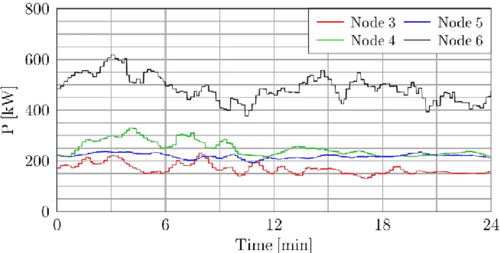
In this section the network with real demand data is analyzed using the Modified Method. The data contains the demands for the day 02/12/2017, which can be seen in Fig. 9. This day was chosen as the demand is lower than usual, which causes low flows in the network increasing the residence time and thus, the losses. The demand is a mixture of residential and commercial buildings gathered every 10 min. The simulation is done with a time step of 60s; values are considered constant during this time. This case study evaluates the network shown in Fig. 5 that contains joints and splits and variable mass flow rates. The time of the simulation for this case study was of 16 min on a medium end computer.
Fig. 9: Demand at every node for the evaluated period.
The behavior of this system was evaluated for three different generation temperatures that remain constant for during the 24 hours being simulated: 90°C, 80°C and 70°C. These temperatures and mode of operation were chosen as they are representative of the operation of some real DH systems. The plant in Node 1 has a larger capacity and provides 65% of the energy while the plant in Node 2 supplies the other 35%. The consumer nodes extract energy from the supply side by deviating part of the mass flow to their own Heat Exchangers and injecting the cooled flow into the return side of the network (Fig. 3). The return temperature ( ) at each heat exchanger is fixed at 40°C,
except on the case of nodes at the end of a branch, where it can be 40°C or higher if there is any surplus energy. To prevent heat waste caused by unnecessary surplus, the mass flows output from the generation units is varied to approximate the power generation with the demand and losses at every time step.
The variables analyzed are the spatial-temporal distribution of the temperature in the network, the mass flow rates, the difference between supply temperature and return temperature at the nodes (Fig.3) (9), and the performance indicator KPI (10).
(9)
(10) This ratio should theoretically be equal to 1, but it will always be higher in reality to compensate for losses. The results for the three temperatures are shown in Figs. 10-12.
4.2.1 Generation at 90°C
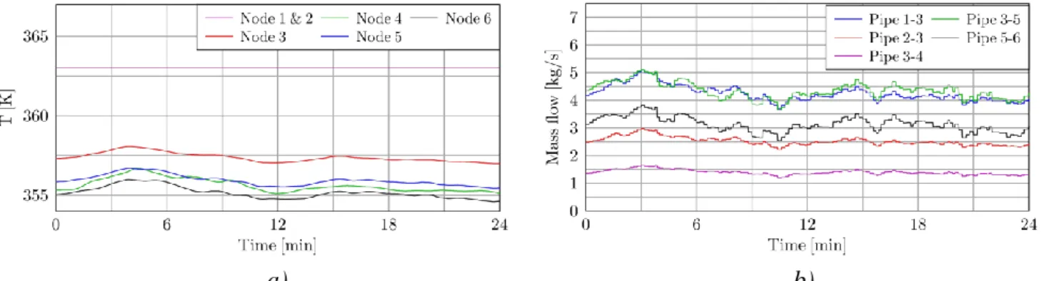
The first simulation was carried out with a generation temperature of 90°C. Fig. 10 shows the spatial-temporal distribution of the temperature at the different nodes and the mass flow rates in the different pipe. The Fig. 11a shows the temperature difference ΔT at every node between the supply and return sides of the network and Fig.11b shows the ratio between the energy generated and the energy demand (KPI).
a) b)
Fig. 10: a) Spatial-Temporal distribution of the temperature in the supply network. b) Mass Flow rates for every pipe in the network (supply and return).
From the Fig. 10 on, it can be seen that the model is able to represent the real dynamics of District Heating networks. In Fig. 10a it can be seen that the farther away the node is from the generation units the lower its available temperature will be. This is caused by the losses that occur during the transport of the heat carrier due to a temperature difference between the hot water and the surroundings. In this case we can see that the losses are very high, as the temperature at the farthest node can be 8°C lower than the generation temperature. This is due to the low mass flows in the network during this day, increasing the residence time of the hot water inside the pipes. Fig. 10b shows that the mass flows vary based on the demand. By comparing the two figures it can be noticed that the losses during transport are not constant and they are decreased when the mass flows increase.
a) b)
Fig. 11: a) Temperature difference between supply and return side at every Node; b) KPI for the two generation nodes and for the entire system.
Fig. 11a shows the temperature difference between the supply and return lines at every node. It can be seen that the highest difference exist at the generation units at around 50°C and the smallest at the farthest away node at 37°C. For Node 1 and 2 the ΔT the variation is under 2°C for most of the system’s operation, but it can be as large as 7°C in Node 4. As Node 4 is at the end of a branch and there are no other downstream nodes after it, any excess of energy it receives will be injected directly into the return line and reduce the ΔT. The variation of the ΔT in Node 4 in this graph indicates that at times there is a surplus of energy and heat is being wasted in the branch 3-4, but it is not noticeable at Nodes 1 and 2 by looking at their ΔT.
Lastly, in Fig. 11b the KPI for the network, as well for each individual generation unit, is shown. It can be seen that even when Node 1 is supposed to supply 65% of the energy and Node 2 35%, the energy waste and the losses provoke that their respective KPI’s are of around 80% and 45%. The arithmetic mean KPI for the system during the 24 hours of operation is of 1.27, which denotes that 27% more energy is being injected into the system than is consumed.
4.2.2 Generation at 80°C & 70°C
The second simulation was made with generation temperature of 80°C and the third with 70°C. The results from these two simulations are summarized and compared with the 90°C simulation in Tables 3-5. Table 3 shows the arithmetic mean of the temperature in every node and the mass flow rate in every pipe. Table 4 shows the arithmetic mean ΔT for every node and the KPI for Nodes 1 and 2 as well as the total for the system. Table 5 shows the standard deviation of the ΔT and KPI shown in Table 4 to give a better understanding of the results.
In Table 3 it is possible to see that for the three cases, the 90°C generation strategy presents the highest temperature drop from the producer nodes to the farthest consumer node (Node 6). This drop is of 7.84 K and is more than double the drop from the 70°C strategy, which is of 3.77 K. It is also visible that in the case of the mass flow rates, the 90°C strategy presents the lowest mass flows while the 70°C has the highest, up to an average of 3.77 kg/s more water circulating in the system.
Node Temperature (K) Pipe Mass Flow (kg/s) 1 2 3 4 5 6 1-3 2-3 3-4 3-5 5-6 90°C 363,00 363,00 357,39 355,64 355,93 355,16 4,25 2,52 1,40 4,35 3,13 80°C 353,00 353,00 349,20 348,02 348,20 347,69 5,42 3,24 1,79 5,58 4,10 70°C 343,00 343,00 340,33 339,48 339,62 339,23 6,57 3,77 2,12 6,57 4,61 Table 3: Arithmetic Mean of Node Temperature and Mass Flow rate for the three generation temperatures.
Because the return temperature at the consumer substations ( ) is fixed at 313 K (except at end of the line nodes), Table 4 shows that the higher the generation temperature the higher the ΔT. But it also shows that the ΔT variation between the production units and the farthest consumer is also higher for greater generation temperatures. For the 90°C case, it can be seen that the ΔT at Node 6 is 13.1K lower than the ΔT at Node 1, but in the case of the 70°C case this difference is only 6.06K. this indicates the higher losses occurring with higher supply temperatures. In this table it is also noticeable that the KPI for the 70°C is 0.06 points better than for the 90°C strategy. This translates to having 6% less waste and losses in the network by generating at a lower temperature.
Δ T (K) KPI
1 2 3 4 5 6 1 2 Total
90°C 50,41 49,78 42,52 41,38 39,99 37,31 0,80 0,47 1,27 80°C 38,88 38,32 33,21 32,79 31,13 28,52 0,79 0,46 1,25 70°C 31,39 31,02 27,26 26,41 26,30 25,33 0,77 0,44 1,21 Table 4: Arithmetic Mean of ΔT and KPI for the three generation temperatures.
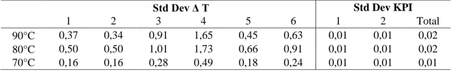
The standard deviation of the results presented in Table 5 gives an interesting insight of the system for the 3 operating strategies. In this table it is possible to notice that for the 90°C and 80°C temperatures the standard deviation in Node 4 is higher than in the other nodes. This may indicate that more energy is being sent to this node than is needed generating waste and lowering the efficiency. As seen in Fig. 11, the losses and mixing in the return network can hide this from the producers if they only monitor their own ΔT.
Std Dev Δ T Std Dev KPI
1 2 3 4 5 6 1 2 Total
90°C 0,37 0,34 0,91 1,65 0,45 0,63 0,01 0,01 0,02 80°C 0,50 0,50 1,01 1,73 0,66 0,91 0,01 0,01 0,02 70°C 0,16 0,16 0,28 0,49 0,18 0,24 0,01 0,01 0,01 Table 5: Standard Deviation of the ΔT’s and KPI’s for the three generation temperatures.
5. Conclusion
This work presented a new modeling approach capable of computing the temperature distribution, in time and space, of a DH system during its operation, as well as the energy flows in the supply and return pipes. Two case studies were analyzed to assess the operation of the model in a 6 node network. The existing FVN method for the Heat Transport in a pipe and the Modified method proposed were also compared for different CFL values.
Results show that, using the electrical analogy to compute the losses and the inertia of the system gives robustness to the model and allows working with fixed spatial discretization for a range of flows, reducing the computation times while keeping accuracy.
With this model it was possible to evaluate the operation of a proposed DH network for a 24 hour with three different generation temperatures and variable energy demand. The results highlight the importance of using tools like the one here presented, as simply knowing the temperatures of the water in the generation nodes is not enough to determine the temperatures and powers in the rest of the network, especially on the far away nodes where any surplus or deficit could be attenuated on the return network and not be noticeable on the generation units.
The results show that even when the temperature and mass flows at the input nodes is known and time series exist to estimate the consumption at the middle nodes, the number of variables and physical phenomena make it hard to know the real-time status of the network without the appropriate tools. This paper presented a new model based on finite volumes to simulate the dynamic response of medium-sized branched DH systems allowing the assessment of the behavior of a DH system beyond the point of view of the generation plants, which are usually the only sites in DH with implemented monitoring. Finite volumes was chosen as it produces the most detailed temperature distribution in a DH network, which is of importance for the applications this model was design for. Some examples are including the design and planning of DH networks; being able to follow the heat train in a network to pinpoint locations for metering, monitoring and energy storage; giving detailed information on the heat available to operate the charge and discharge of heat storage; giving instantaneous information on the QoS.
The results show the relevance of having monitoring along the network and justify the use of ICTs for monitoring and optimal control. This model can support the incorporation of monitoring, communication and control strategies to evaluate the energy and economic performance of DH as Smart Thermal Networks.
Acknowledgments
The research presented is performed within the framework of the Erasmus Mundus Joint Doctorate SELECT+ program ‘Environomical Pathways for Sustainable Energy Services’ and funded with support from the Education, Audiovisual, and Culture Executive Agency (EACEA) (Nr 2012-0034) of the European Commission. Support from the IN+ strategic Project UID/EEA/50009/2013 is gratefully acknowledged. This publication reflects the views only of the author(s), and the Commission cannot be held responsible for any use, which may be made of the information contained therein.
Nomenclature
Roman letters CFL Courant-Friedrich-Levy condition Cp specific heat, J/(kg K) DW head loss, m d diameter, m e effective roughness, mm f friction factor g gravity, m/s2 k thermal conductivity, W/(m K) L pipe length, m .m mass flow rate, kg/s R thermal resistance, K/W T temperature, K t time, s u flow speed, m/s V volume, m3 Greek symbols density, kg/m3 pipe diameter, mm Subscripts and superscripts a ambient D demand i time index in inflow ins insulation j spatial index
loss losses to the surroundings out outflow r return s supply soil soil st steel sub substation vol control volume w water
References
[1] Bouhafs F, Mackay M, Merabti M. Links to the Future: Communication Requirements and Challenges in the Smart Grid. IEEE Power Energy Mag. 2012;10:24–32.
[2] Zheng J, Zhou Z, Zhao J, et al. Function method for dynamic temperature simulation of district heating network. Appl. Therm. Eng. 2017;123:682–688.
[3] Vesterlund M, Toffolo A, Dahl J. Optimization of multi-source complex district heating network, a case study. Energy. 2017;126:53–63.
[4] Mazhar AR, Liu S, Shukla A. A state of art review on the district heating systems. Renew. Sustain. Energy Rev. 2018;96:420–439.
[5] Niemi R, Mikkola J, Lund PD. Urban energy systems with smart multi-carrier energy networks and renewable energy generation. Renew. Energy. 2012;48:524–536.
[6] Buffa S, Cozzini M, D’Antoni M, et al. 5th generation district heating and cooling systems: A review of existing cases in Europe. Renew. Sustain. Energy Rev. 2019;104:504–522.
[7] Crispim J, Braz J, Castro R, et al. Smart Grids in the EU with smart regulation: Experiences from the UK, Italy and Portugal. Util. Policy. 2014;31:85–93.
[8] Koliou E, Bartusch C, Picciariello A, et al. Quantifying distribution-system operators’ economic incentives to promote residential demand response. Util. Policy. 2015;35:28–40.
[9] Rocha P, Siddiqui A, Stadler M. Improving energy efficiency via smart building energy management systems: A comparison with policy measures. Energy Build. 2015;88:203–213. [10] Xue X, Wang S, Sun Y, et al. An interactive building power demand management strategy
for facilitating smart grid optimization. Appl. Energy. 2014;116:297–310.
[11] Wissner M. The Smart Grid – A saucerful of secrets? Appl. Energy. 2011;88:2509–2518. [12] Lund H, Werner S, Wiltshire R, et al. 4th Generation District Heating (4GDH): Integrating
smart thermal grids into future sustainable energy systems. Energy. 2014;68:1–11.
[13] Gungor V c., Sahin D, Kocak T, et al. Smart Grid Technologies: Communication Technologies and Standards. IEEE Trans. Ind. Inform. 2011;7:529–539.
[14] del Hoyo Arce I, Herrero López S, López Perez S, et al. Models for fast modelling of district heating and cooling networks. Renew. Sustain. Energy Rev. 2018;82:1863–1873.
[15] Bahramipanah M, Cherkaoui R, Paolone M. Decentralized voltage control of clustered active distribution network by means of energy storage systems. Electr. Power Syst. Res. 2016;136:370–382.
[16] Mancarella P. MES (multi-energy systems): An overview of concepts and evaluation models. Energy. 2014;65:1–17.
[17] Larsen HV, Bøhm B, Wigbels M. A comparison of aggregated models for simulation and operational optimisation of district heating networks. Energy Convers. Manag. 2004;45:1119–1139.
[18] A stable and accurate convective modelling procedure based on quadratic upstream interpolation - ScienceDirect [Internet]. [cited 2019 Apr 12]. Available from: https://www.sciencedirect.com/science/article/pii/0045782579900343.
[19] Benonysson A. Dynamic modelling and operational optimization of district heating systems. Lyngby, Techn. Univ. of Denmark, Ph. D. Thesis; 1991.
[20] Gabrielaitiene I, Bøhm B, Sunden B. Evaluation of Approaches for Modeling Temperature Wave Propagation in District Heating Pipelines. Heat Transf. Eng. 2008;29:45–56.
[21] Gabrielaitiene I, Bøhm B, Sunden B. Modelling temperature dynamics of a district heating system in Naestved, Denmark—A case study. Energy Convers. Manag. 2007;48:78–86.
[22] Gabrielaitienė I, Bøhm B, Sundén B. Dynamic temperature simulation in district heating systems in Denmark regarding pronounced transient behaviour / Danijos šilumos tiekimo sistemų modeliavimas, įvertinant nestacionarų temperatūros pasiskirstymą tinkle. J. Civ. Eng. Manag. 2011;17:79–87.
[23] Stevanovic VD, Jovanovic ZLj. A hybrid method for the numerical prediction of enthalpy transport in fluid flow - ScienceDirect. Int. Commun. Heat Mass Transf. 2000;27:23–34.
[24] Stevanovic VD, Zivkovic B, Prica S, et al. Prediction of thermal transients in district heating systems. Energy Convers. Manag. 2009;50:2167–2173.
[25] Zhou S, Tian M, Zhao Y, et al. Dynamic modeling of thermal conditions for hot-water district-heating networks. J. Hydrodyn. Ser B. 2014;26:531–537.
[26] Dénarié A, Aprile M, Motta M. Heat transmission over long pipes: New model for fast and accurate district heating simulations. Energy. 2019;166:267–276.
[27] Yuan X, Yali X, Qiongyao W. Dynamic temperature model of district heating system based on operation data. Energy Procedia. 2019;158:6570–6575.
[28] Hohmann M, Warrington J, Lygeros J. A two-stage polynomial approach to stochastic optimization of district heating networks. Sustain. Energy Grids Netw. 2019;17:100177.
[29] Wang Y, You S, Zhang H, et al. Thermal transient prediction of district heating pipeline: Optimal selection of the time and spatial steps for fast and accurate calculation. Appl. Energy. 2017;206:900–910.
[30] Sartor K, Thomas D, Dewallef P. A comparative study for simulation of heat transport in large district heating network [Internet]. 2015 [cited 2018 Jan 29]. Available from: https://orbi.uliege.be/handle/2268/183406.
[31] Oppelt T, Urbaneck T, Gross U, et al. Dynamic thermo-hydraulic model of district cooling networks. Appl. Therm. Eng. 2016;102:336–345.
[32] van der Heijde B, Fuchs M, Ribas Tugores C, et al. Dynamic equation-based thermo-hydraulic pipe model for district heating and cooling systems. Energy Convers. Manag. 2017;151:158–169.
[33] Lim S, Park S, Chung H, et al. Dynamic modeling of building heat network system using Simulink. Appl. Therm. Eng. 2015;84:375–389.
[34] Lawson DI, McGuire JH. The Solution of Transient Heat-flow Problems by Analogous Electrical Networks. Proc. Inst. Mech. Eng. 1953;167:275–290.
[35] Katsuhiko Ogata. System Dynamics. 4th ed. University of Minnesota: Pearson; 2004.
[36] Marguerite C, Bourges B, Lacarrière B. Application of a Districy Heating Network (DHN) Model for an ex-ante Evaluation to Support a Multi-Source DH [Internet]. Int. Build. Perform. Simul. Assoc. 2013 [cited 2017 Mar 8]. Available from: http://www.ibpsa.org/proceedings/BS2013/p_2433.pdf.
[37] Barr D. Technical note. two additional methods of direct solution of the colebrook-white function. Proc. Inst. Civ. Eng. 1975;59:827–835.
Annex A
CFL
Spatial Discretization
m
Pipe 1-3 Pipe 2-3 Pipe 3-4 Pipe 3-5 Pipe 5-6 1.00 14.60 10.97 10.40 15.19 15.19 0.95 15.40 11.55 10.95 15.99 15.99 0.75 19.50 14.63 13.86 20.26 20.26 0.50 29.26 21.94 20.82 30.38 30.38 0.30 48.76 36.57 34.7 50.64 50.64