Demand Forecasting Using
Monte Carlo Multi-Attribute Utility Theory By
John Stefancik
B.S.M.E. Mechanical Engineering, University of Mississippi (2014)
Submitted to the Institute for Data, Systems, and Society in partial fulfillment of the requirements for the degree of
Master of Science in Technology and Policy at the
MASSACHUSETTS INSTITUTE OF TECHNOLOGY June 2016
Massachusetts Institute of Technology 2016. All rights reserved.
Author...
S ig n a tu re re d a c te d
Institute for Data, Systems, and Society May 12, 2016
Signature
redacted
C e rtifie d b y ... .. :... Richard Roth Research Associate Thesis AdvisorSignature redacted
A cce p te d b y ... Munther Dahleh William A. Coolidge Professor of Electrical Engineering and Computer Science Acting Director, Technology and Policy Program MnSACHUSTS INSTITUTE Director, Institute for Data, Systems, and SocietyOF TECHNOLOGY
JUN 14 Z016
LIBRARIES
ARCHVE8
Demand Forecasting Using
Monte Carlo Multi-Attribute Utility Theory By
John Stefancik
Submitted to the Institute for Data, Systems, and Society on May 12, 2016 in Partial Fulfillment of the Requirements for the Degree of Master of Science in
Technology and Policy
ABSTRACT
Volatile commodity prices over the past decade, environmentally-focused policy initiatives and new technology developments have forced manufacturers to consider the idea of substituting towards alternative materials in order meet both consumer and societal needs. The threat of substitution has created the need for manufacturing firms and other members of the supply chain to have the ability to understand the implications of substitution on future product market shares and overall raw material demand.
This thesis demonstrates how Multi-Attribute Utility Theory (MAUT) can be extended to the group level to forecast future market shares by applying a distribution to the attribute weights and using a Monte Carlo simulation to capture the choices made by a heterogeneous set of decision makers. Unlike established demand forecasting techniques, such as discrete choice models, this methodology requires only a few data points from a handful of expert interviews and allows for systematic changes of preferences over time. Furthermore, the Monte Carlo MAUT methodology utilizes both revealed preference and stated preference data by integrating the two data types through a response surface methodology.
Two case studies on underground distribution and overhead distribution power cables are explored in order to illustrate how the Monte Carlo MAUT methodology can be successfully applied in cases where there are diverse product types, limited numbers of decisions makers and historical market share data is sparse. Each case study illustrates how Monte Carlo MAUT can, on a regional basis, provide key insights into the impacts of changing commodity prices, changing product attribute levels, varying new technology learning rates and changing consumer preferences over time. Furthermore, an example of how Monte Carlo MAUT can be utilized to help policymakers evaluate the advantages, disadvantages and overall impact of different policy schemes within an environmental context is provided.
Private firms and public governments alike can utilize Monte Carlo MAUT to improve their understanding of how market shares are likely to change over time, and more importantly, the key decisions needed on each party's behalf in order to maximize societal well-being.
Thesis Supervisor: Richard Roth Title: Research Associate
Acknowledgements
Where to begin? It's been quite the ride and experience from September 2014 until now. I came to MIT looking to expand my horizons and put myself in a position to begin my professional career. I can safely say I've accomplished both of those goals. Beyond that, I didn't really know what to expect. Looking back at the past 21 months, I've learned a myriad of technical, emotional, social and societal lessons that I will carry with me forever. MIT and TPP have changed the way I think, my understanding of how the world works and helped me formulate what I want to do with my life. This has experience has opened doors that I didn't know existed and developed skills I didn't know I had. For these reasons, I am eternally grateful for the opportunity to be a member of TPP.
The first person that deserves recognition is Frank Field. Frank has had either a direct or indirect role in pretty much my entire TPP experience. From his critiques and comments on research to his administrative role as TPP Director of Education, Frank has helped me find a research home at MSL and made the administrative portion of the program simple from the student perspective. Coming from a family without any Ph.Ds or research centric degrees, Frank has always made sure my southern self has found a way to enjoy my time at MIT. From a personal perspective, I am very grateful.
Rich Roth has been a tremendous advisor and a person I am proud to call my friend. From research discussions to running through LAX Amazing Race Style to celebrating Pride in London to our random yet inevitable discussions about Memphis and life in general, it has been a pleasure working together. I look forward to continuing our friendship and eventually crashing in a spare bedroom in San Diego sometime after February 20, 2019.
My research experience would not be possible if not for the support of Mike Harris and the Economics and Markets Team at Rio Tinto. You guys provided me with one hell of an experience that included a week in Australia and a summer in London. So much of my learning experience has been a unique result of working with y'all. I thoroughly enjoyed our time together and hope that this thesis helps contribute today and leads to further contributions in the future.
To all my colleagues in MSL, it has been a pleasure working alongside and learning from each of you. I'm excited to see what the future holds for all of you as I am confident that everyone will accomplish their goals and fulfill their ambitions.
A special acknowledge goes to my friend and former colleague Nathan Kerns. Nathan developed the design cost model used to calculate several of the Upfront Cost attribute levels in this thesis. He certainly deserves recognition for his contribution. Hopefully this work is worthy of you association.
Being a member of TPP has been a wonderful experience, and the friendships I've built with my TPP colleagues have been the best part of the experience. I look forward to keeping in touch with
everyone and witnessing the great accomplishments of our class in the future. Additionally, I'd be remiss not to acknowledge the work Barb, Ed and Noelle do as administrators in order to make our lives as students as enjoyable as possible.
A key component to a successful TPP experience is great roommates. I've had the honor of living with two fantastic sets of roommates: 'Murica house with Alex, Chris, Jacob and Justin and the Danger Zone with John and Turner. I'm looking forward to our future reunions in New Orleans and anywhere else we deem worthy of our presence.
Finally, I'd like to thank Mom, Dad, Sara and Hannah for their support the past couple of years. You've helped maintain my sanity, and I am very grateful. I look forward to celebrating my graduation from MIT and sharing future endeavors with all of you.
Table of Contents
1 Introduction ... 16
1.1 Existing Forecasting M ethodologies ... 16
1.2 Research Question ... 18
2 M ethodology: M onte Carlo M ulti-Attribute Utility Theory ... 19
2.1 M ulti-Attribute Utility Theory at the Individual Level ... 19
2.2 M ulti-Attribute Utility Theory Extended to the Group Level... 21
2.3 Applying M onte Carlo M AUT Over Tim e ... 25
2.4 Revealed Preferences and Stated Preferences... 26
2.5 Determining the Set of Ratings using Revealed Preference (Market Share) Information...27
2.6 Translating Modelled or "Target" Market Shares into Actual Market Shares... 30
3 Case Study Overview : Pow er Cables... 31
3.1 Overview of Pow er Cables ... 31
3.1.1: Functional Unit Discussion and Definition... 33
3.2 Alternative Set ... 34
3.3 Attribute Set...36
3.4 Single Utility Functions... 40
3.5 M ulti-attribute Utility Functions ... 43
4 Case Study: Underground Distribution ... 44
4.1 Defining the Functional Unit ... 45
4.2 North Am erica Baseline Scenario ... 46
4.2.1 Attri bute Levels ... 46
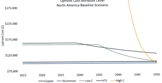
4.2.1.1 Upfront Cost ... 47
4.2.1.2 Operating Cost ... 51
4.2.1.3 System Reliability ... 53
4.2.1.4 Tech Fam iliarity ... 54
4.2.2 Single Utility Function Coefficients ... 55
4.2.3 Determ ining the Initial W eights for the M UF ... 56
4.2.4 Utility Scores and M arket Share Forecasts ... 59
4.4 W hat if Technology Learning is Faster? ... 65
4.5 Preference Sensitivities...67
4.6 Key Regional Sensitivities... 75
4 .6 .1 In d ia ... 7 8 4 .6 .2 C h in a ... 8 2 4.6.3 Com parisons Between North Am erica, India & China Regions ... 85
5 Case Study: Overhead Distribution ... 90
5.1 Definitions & Ratings...90
5.2 North Am erica Baseline Scenario ... 91
5.2.1 Attribute Levels ... 91
5.2.1.1 Upfront Cost...92
5.2.1.2 Operating Cost ... 96
5.2.1.3 System Reliability ... 98
5.2.1.4 Tech Fam iliarity ... 99
5.2.2 Single Utility Function Coefficients ... 100
5.2.3 Determ ining the Initial W eights for the M UF ... 101
5.2.4 Utility Scores and M arket Share Forecasts ... 103
5.3 P rice Sensitivity ... 105
5.4 W hat if Technology Learning is Faster?...107
5.5 Key Preference Sensitivities ... 108
5.6 Key Regional Sensitivities... 111
5 .6 .1 In d ia ... 1 1 3 5.6.2 China ... 116
5.6.3 Com parisons Between North Am erica, India & China Regions ... 119
6 Com bining M onte Carlo M AUT & Policy...124
6.1 Baseline Carbon Footprint per North America Underground Distribution Functional Unit...124
6.2 Environm ental Policy Scenarios ... 126
6.2.1: Car bon Tax ... 126
6.2.2 Subsidies ... 128
6.2.3 Com parison of M echanism s...130
6.3 Prom oting Increase in Underground versus Overhead Distribution System s...131
7 Conclusions & Future W ork ... 135 7
Appendix ... 138
Appendix A: Sam ple Survey ... 138
Appendix B: Underground Distribution Sub-attribute Levels...141
Appendix C: Deployment Cost & Finished Cable Cost Methodology, Assumptions & Calculations...144
C.1 Deploym e nt Cost ... 144
C.2 Finished Ca ble Cost ... 146
Appendix D: Operating Cost Calculation M ethodology ... 156
Appendix E: Overhead Distribution Sub-attribute Levels ... 159
Appendix F: Deployment Cost & Finished Cable Cost Methodology, Assumptions & Calculations. Overhea d Distribution ... 162
F.1 Deploym ent Cost...162
F.2 Finished Ca ble Cost ... 164
List of Figures & Tables
Table 2.2: Sum m ary of beta distribution spread criteria... 23
Figure 2.2a: Beta distribution (left) and truncated beta distribution (right)... 24
Figure 2.2b: Hypothetical Monte Carlo MAUT example. The vertical line represents where the trials go from negative to positive y-axis values (Utility of Alternative 1 - Utility of Alternative 2)...24
Figure 2.3a: Hypothetical binary case between and incumbent technology and a new technology. As the new technology gains utility over time (left graph), it begins to take market share from the incumbent tech no lo gy (rig ht g ra p h). ... 2 5 Figure 2.3b: Hypothetical binary case between and incumbent technology and a new technology where preferences change over tim e... 26
Figure 2.5: Graphical representation of initial rating set determination method. The horizontal axis is attribute 1 and the vertical axis is attribute 2. ... 29
Figure 3.1: Common concentric 3 phase power cable design. ... 33
Figure 3.4a: Upfront Cost single attribute functional form: negative exponential (Ae - B * x)...41
Figure 3.4b: Tech Fam iliarity Single Utility Function. ... 42
Table 3.4: Summary of Single Attribute Utility Functional Forms ... 42
Table 4.1: Material Intensities and Resistances for Underground Distribution Alternative Set ... 46
Figure 4.2.1.1a: Baseline Scenario global price forecasts for copper and aluminum...47
Table 4.2.1.1a: Average Conductor Material Price (Non-Cu/Al) initial cost levels and learning rates. North A m erica U nderground D istribution...48
Figure 4.2.1.1b: Average Material Price (Non Cu/Al) sub-attribute level from 2015-2050 in the North A m e rica baseline scenario.. ... 48
Table 4.2.1.1b: Alloying and Semi-fabrication Cost initial values and learning rates. North America U nd e rgro u nd D istribution ... 4 9 Figure 4.2.1.1c: Alloying & Semi-fab cost sub-attribute level from 2015-2050 in the North America b ase lin e sce na rio. ... 4 9 Table 4.2.1.1c: Finished Cable (Cabling) Cost and Deployment Cost sub-attribute levels for each alternative. North Am erica Underground Distribution. ... 50
Table 4.2.1.1d: 2015 Upfront Cost attribute levels. North America Underground Distribution...50 Figure 4.2.1.1d: Upfront Cost attribute level from 2015-2050 for all alternatives in the North America b ase line sce na rio. ... 5 1 Table 4.2.1.2: Operating Cost attribute level from 2015-2050 for all alternatives in the North America
B a se lin e S ce n a rio ... 5 2
Table 4.2.1.3: 2015 System Reliability attribute level and learning rates for all alternatives in the North A m erica Baseline Scenario... 53 Figure 4.2.1.3: System Reliability attribute level from 2015-2050 for all alternatives in the North America B a se lin e S ce n a rio ... 5 4
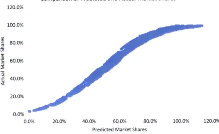
Table 4.2.1.4: 2015 Tech Familiarity Attribute levels. North America Underground Distribution...55 Table 4.2.1: 2015 Attribute levels for the Baseline North America Underground Distribution scenario .. 55 Table 4.2.2: SUF Coefficients and Attribute Level Ranges. Underground Distribution...56 Table 4.2.3a: Summary statistics for the North America underground distribution response surface. D istributio n spread of +/- 3... 57 Figure 4.2.3: Actual market shares versus predicted market shares via the response surface equation for the Copper alternative in North Am erica. ... 58
Table 4.2.3b: Initial Attribute Ratings (Ri) and Normalized Weights (wi) for North America
U nde rgro u nd D istributio n ... 58
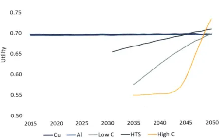
Figure 4.2.4a: Mean utility values for all 5 alternatives from 2015-2050 in the North America baseline sc e n a rio ... 5 9
Table 4.2.4: 2025, 2035 and 2045 trial samples. North America Underground Distribution ... 61
Figure 4.2.4b: Comparison of Copper and HTS Utility Bands for the North America baseline scenario.... 62 Figure 4.2.4c: Market Shares (left) for each alternative from 2015-2050 and Overall Material Intensities (right) for Copper and Aluminum in the North America baseline scenario...62 Figure 4.3a: Price strings utilized in price sensitivity scenario (baseline and 20% increases)...63 Figure 4.3b: Copper market share for the baseline, 20% Cu price increase and 20% Al price increase sce n a rio s...6 4
Figure 4.3c: Summary Price Sensitivity Relative Intensity graphs for Copper (left) and Aluminum (right). ... 6 4
Figure 4.4a: Comparison of Baseline Average Material Price (non Cu/Al) learning in the baseline scenario and the 40% increased learning scenario (left) and Semi-fab Cost learning in the baseline and increased
learning scenario (right) for Low C, HTS and High C. ... 66
Table 4.4a: 2050 Market Share Scenarios where Nanotubes and HTS learn independently... 66 Table 4.4b: 2050 Market Share Scenarios where Nanotubes and HTS learn together. ... 67
Figure 4.5a: Market share comparison between baseline scenario (Upfront Cost rating is a constant 7.99) and increasing the Upfront Cost rating from 7.99 (baseline) to 8.99 incrementally from 2015 to 2025... 69 Figure 4.5b: Market share comparison between baseline scenario (Upfront Cost rating is a constant 7.99) and decreasing the Upfront Cost rating from 7.99 to 6.99 incrementally from 2015 to 2025...69
Figure 4.5c: Summary of Material Intensities for Copper (left) and Aluminum (right) for the baseline, Upfront Cost rating increase and Upfront Cost rating decrease sensitivity scenarios...70 Figure 4.5d: Comparison of Material Intensities for Copper and Aluminum in the Baseline Scenario and the Increase in System Reliability rating scenario. ... 72
Figure 4.5e: Comparison of copper, aluminum and HTS market shares between the baseline, tech familiarity rating increasing and tech familiarity rating decreasing scenarios...73
Figure 4.5f: Summary of Material Intensities for Copper (left) and Aluminum (right) for the baseline, Tech Familiarity rating increase and Tech Familiarity rating decrease sensitivity scenarios. North America
R e g io n . ... 7 4
Table 4.6a: Initial Attribute Ratings (Ri) and Normalized Weights (wi) for India Underground
D istrib u tio n ... 7 6
Table 4.6b: Summary statistics for the China underground distribution response surface. Distribution sp re a d o f + /- 4...7 6
Table 4.6b: Initial Attribute Ratings (Ri) and Normalized Weights (wi) for China Underground
D istrib u tio n ... 7 7
Table 4.6c: Summary of Attribute Ratings across North America, India and China. ... 77
Figure 4.6.1a: Baseline Market Share forecast and Overall Material Intensity forecast for India. ... 78
Figure 4.6.1b: Comparison of copper market shares when long term (2026-2050) copper price increases 20% and decreases 20% in the India Underground Distribution market. ... 79
Figure 4.6.1c: Summary of Material Intensities for Copper (left) and Aluminum (right) for the Price Sensitivity Scenarios. India Region... 79
Figure 4.6.1d: Market share comparison for copper, aluminum and HTS between baseline scenario (Upfront Cost rating is a constant 9.43) and decreasing the Upfront Cost rating from 9.43 to 8.43
increm entally from 2015 to 2025. India Region. ... 80
Figure 4.6.1e: Comparison of Material Intensities for Copper and Aluminum in the Baseline Scenario and the decrease in Upfront Cost rating scenario... 81
Figure 4.6.1f: Comparison of Material Intensities for Copper and Aluminum in the Baseline Scenario and the increase in System Reliability rating scenario. ... 82
Figure 4.6.2a: Baseline Market Share forecast and overall Material Intensity forecast for China
U nd e rg ro u nd D istributio n...8 2
Figure 4.6.2b: Comparison of copper market shares when long term (2026-2050) copper price increases 20% and decreases 20% in the China Underground Distribution market. ... 83
Figure 4.6.2c: Summary of Material Intensities for Copper (left) and Aluminum (right) for the Price Sensitivity Scenarios. C hina Region. ... 83
Figure 4.6.2d: Market share comparison between baseline scenario (Operating Cost rating is a constant 5.40) and increasing the Operating Cost rating from 5.40 to 6.40 incrementally from 2015 to 2025. China
R e g io n . ... 8 4
Figure 4.6.2e: Comparison of Material Intensities for Copper and Aluminum in the Baseline Scenario and the increase in Operating Cost rating scenario... 85
Figure 4.6.3a: Summary of Copper and Aluminum market shares and material intensities for the baseline scenario in each region. Underground Distribution. ... 86
Figure 4.6.3b: Comparison of copper market shares in the baseline (constant preferences) and changing preferences scenarios across all three regions. Underground Distribution...87 Table 4.6.3a: Comparison of 2035 Copper Material Intensity in the Baseline and 20% Cu Price Increase
scenarios. U nderground Distribution. ... 88
Table 4.6.3b: Comparison of the 2050 Copper and Aluminum Material Intensities in the Baseline
scenario and Incumbents Only scenario. Underground Distribution. ... 88
Table 5.1: Material Intensities and Resistances for the Overhead Distribution Alternative Set...91 Figure 5.2.1.1a: Baseline Scenario global price forecasts for copper and aluminum...93 Table 5.2.1.1a: Average Conductor Material Price (Non-Cu/Al) initial cost levels and learning rates. North
A m erica O verhead D istribution...93 Figure 5.2.1.1b: Average Material Price (Non Cu/Al) sub-attribute level from 2015-2050 in the North A m e rica base line sce nario . ... 9 3
Table 5.2.1.1b: Alloying and Semi-fabrication Cost initial values and learning rates. North America
O ve rhead D istributio n. ... 94
Figure 5.2.1.1c: Alloying & Semi-fab cost sub-attribute level from 2015-2050 in the North America
base line sce n a rio. ... 9 4
Table 5.2.1.1c: Finished Cable (Cabling) Cost and Deployment Cost sub-attribute levels for each
alternative. North Am erica Overhead Distribution. ... 95
Table 5.2.1.1d: 2015 Upfront Cost attribute levels. North America Underground Distribution...95 Figure 5.2.1.1d: Upfront Cost attribute level from 2015-2050 for all alternatives in the North America baseline scenario. Overhead Distribution... 96
Table 5.2.1.2: Operating Cost attribute level from 2015-2050 for all alternatives in the North America Baseline Scenario. Overhead Distribution. ... 97
Table 5.2.1.3: 2015 System Reliability attribute level and learning rates for all alternatives in the North A m erica Baseline Scenario... 98 Figure 5.2.1.3: System Reliability attribute level from 2015-2050 for all alternatives in the North America B ase lin e Sce n a rio ... 9 9
Table 5.2.1: 2015 Attribute levels for the Baseline North America Overhead Distribution scenario ... 100
Table 5.2.2: SUF Coefficients and Attribute Level Ranges. Underground Distribution...101 Table 5.2.3a: Summary statistics for the North America overhead distribution response surface.
D istributio n spread of +/- 4 ... 102
Figure 5.2.3: Actual market shares versus predicted market shares via the response surface equation for the Copper alternative in North Am erica. ... 102
Table 5.2.3b: Initial Attribute Ratings (Ri) and Normalized Weights (wi) for North America Overhead
D istrib u tio n ... 1 0 3
Figure 5.2.4a: Mean utility values for all 4 alternatives from 2015-2050 in the North America baseline sc e n a rio ... 1 0 4
Figure 5.2.4b: Market Shares (left) for each alternative from 2015-2050 and Overall Material Intensities (right) for Copper and Aluminum in the North America baseline scenario...105 Figure 5.3a: Comparison of aluminum market shares when long term (2026-2050) copper price increases 20% (left) and decreases 20% (right) in the North America Overhead Distribution market...106 Figure 5.3b: Summary of Material Intensities for Copper (left) and Aluminum (right) for the Price
Sensitivity Scenarios. North Am erica Overhead Distribution...106 Figure 5.4a: Comparison of Baseline Average Material Price (non Cu/Al) learning (left) and Alloying & Semi-fabrication cost learning (right) in the baseline scenario and the 40% increased learning rate
scenario fo r Low C and H igh C. ... 107
Table 5.4a: 2050 Market Share Scenarios. North American Overhead Distribution...108 Figure 5.5a: Market share comparison between baseline scenario (Operating Cost rating is a constant
5.53) and increasing the Operating Cost rating from 5.53 to 6.53 incrementally from 2015 to 2025. North
A m e rica R eg io n ... 10 9
Figure 5.5b: Comparison of'Material Intensities for Copper and Aluminum in the Baseline Scenario and the increase in O perating Cost rating scenario...110
Figure 5.5c: Material Intensity comparison between baseline scenario (System Reliability rating is a constant 5.53) and increasing the System Reliability rating from 5.53 to 7.53 incrementally from 2015 to
2025. N o rth A m erica Regio n...110
Table 5.6a: Initial Attribute Ratings (Ri) and Normalized Weights (wi) for India Overhead Distribution ... 1 1 2
Table 5.6b: Initial Attribute Ratings (Ri) and Normalized Weights (wi) for India Overhead Distribution ... 1 1 2
Table 5.6c: Summary of Attribute Ratings across North America, India and China. ... 113
Figure 5.6.1a: Baseline Market Share forecast and Overall Material Intensity forecast for India. ... 114
Figure 5.6.1b: Comparison of Material Intensities when long term (2026-2050) copper price increases 20% (left) and decreases 20% (right) in the India Overhead Distribution market. ... 114 Figure 5.6.1d: Market share comparison between baseline scenario (Upfront Cost rating is a constant
9.03) and decreasing the Upfront Cost rating from 9.03 to 8.03 incrementally from 2015 to 2025. India
R e g io n . ... 1 1 5
Figure 5.6.1e: Comparison of Material Intensities for Copper and Aluminum in the Baseline Scenario and the decrease in Upfront Cost rating scenario...116 Figure 5.6.2a: Baseline Market Share forecast and overall Material Intensity forecast for China Overhead D istrib u tio n ... 1 1 7
Figure 5.6.2b: Comparison of Material Intensities when long term (2026-2050) copper price increases 20% (left) and decreases 20% (right) in the China Overhead Distribution market. ... 117
Figure 5.6.2d: Market share comparison between baseline scenario (Operating Cost rating is a constant 4.15) and increasing the Operating Cost rating from 4.15 to 5.15 incrementally from 2015 to 2025. China R e g io n . ... 1 1 8
Figure 5.6.2e: Comparison of Material Intensities for Copper and Aluminum in the Baseline Scenario and the increase in O perating Cost rating scenario...119 Figure 5.6.3a: Summary of Copper and Aluminum market shares and material intensities for the baseline scenario in each region. Overhead Distribution. ... 120
Figure 5.6.3b: Comparison of copper market shares in the baseline (constant preferences) and changing preferences scenarios across all three regions. Overhead Distribution...121 Table 5.6.3a: Comparison of 2035 Copper Material Intensity in the Baseline and 20% Cu Price Increase scenarios. O verhead D istribution. ... 121 Table 5.6.3b: Comparison of the 2050 Copper and Aluminum Material Intensities in the Baseline
scenario and Incum bents Only scenario. Overhead Distribution. ... 122
Figure 6.1a: Comparison of Year 1 (the year a functional unit is installed and begins operation) CO2
emissions between the Copper and Aluminum underground distribution alternatives...125
Figure 6.1b: Summary of CO2 emissions from losses in the North American underground distribution
b a se lin e sce n a rio. ... 12 6 Table 6.2: Comparison of Operating Cost Attribute Levels with and without a Carbon Tax...127
Figure 6.2a: Impact of carbon tax on copper and aluminum prices (left graph) and the operating cost attribute levels (right graph)... 128
Figure 6.2b: Comparison of baseline and carbon tax scenarios for copper, aluminum and HTS market s h a re s ... 1 2 8
Figure 6.2d: Comparison of market share forecasts between the baseline scenario and the subsidy scenario for North Am erica Underground Distribution...130 Figure 6.2e: Comparison of Overall Material Intensities for Copper (left) and Aluminum (right) in the baseline, carbon tax and subsidy scenarios...130 Figure 6.2f: Comparison of Total CO2 Emissions from operating losses in the baseline, carbon tax and su bsid y sce n a rio s. ... 13 1 Figure 6.3a: Comparison of Distribution Network market between today's 48% underground/52% overhead split and a hypothetical 70% underground/30% overhead split...132
Figure 6.3b: Relative intensities of copper and aluminum in a scenario where underground distribution's share of the total distribution market rises from 48% in 2015 to 70% in 2030. ... 133
Figure 6.3c: Comparison of total CO2 emissions from losses at 48% underground (today's share) and 70%
undergro und (hypothetical)...134
1
Introduction
From 2010 to 2012, multiple commodities, including oil, iron ore and thermal coal reached historically high price levels, primarily as a result of China experiencing a decade of robust growth and development. Copper in particular benefitted tremendously from China's rapid growth, as evidenced by copper prices exceeding $4.00/lb in 2011, which was approximately 4 times higher
than the customary $1.00/lb price seen consistently in the early 2000s1.
Soaring commodity prices, in combination with a global economy still recovering from the 2008 Global Financial Crisis, sparked several manufacturers to explore the viability of replacing expensive raw materials (such as copper) for less expensive raw materials (such as aluminum) in product categories where either material was capable of meeting customer requirements. Simultaneously, global policymakers have become increasingly interested in developing policies that reduce greenhouse gas emissions as part of their efforts to curb the adverse effects of global warming. Tangible evidence of this phenomena exists; for example, Ford has transitioned from steel to aluminum as the primary material in their F150 pickup in response to stricter Corporate Average Fuel Economy requirements being implemented progressively until 2025.
The development of new material technologies also poses a threat to the current equilibrium of material usage in several product sectors. This source of substitution is a combination of both technology firms seeking to penetrate existing markets for capitalistic reasons as well as government policies being crafted to facilitate the development of advanced technologies for sustainability reasons.
The combination of uncertainty about future material prices, government policy initiatives and new material technology developments accentuates the need for a forecasting methodology that can provide insight into the future market shares of both incumbent and new technology alternatives. This information can be utilized by both the private sector and policymakers alike in making optimal decisions from a materials consumption perspective.
1.1 Existing Forecasting Methodologies
Forecasting market shares has been a topic of interest to business managers and academics alike for decades. Historically, two sets of methodologies have been utilized across a breadth of applications: Conjoint Analysis and Discrete Choice Models. Conjoint Analysis is a market research technique based on estimations of the structure of consumer evaluations on a set of alternatives consisting of predetermined combinations of product attribute levels (Asioli et al.
2016). Consumer preferences are revealed through evaluations of the buyers' tradeoffs among the multiple attributes of the alternatives. Conjoint analyses are particular useful for ranking the importance of attributes as well as determining a consumer's marginal willingness to pay. These insights make Conjoint Analysis an appealing method to both academic and corporate researchers alike (Rao 2014).
Traditional Discrete Choice models assume an individual's decision making process is based on utility maximization. The utility can be modeled as a function of observable attributes as well as the individual's socioeconomic data. Discrete Choice models assume that the individual's decision making process is well captured by the model by virtue of the presumed link between the observable attributes (inputs) and the choice data (outputs) (Danthurebandara, Vandebroek, and Yu 2013). The choice data for multiple respondents can be transformed into a choice probability through a statistical fit of the choice data. The most common technique is Logit, which offers a closed form solution to finding choice probabilities by virtue of its assumption that unobserved attributes are uncorrelated across all alternatives. While restrictive, Logit is analytically convenient and solvable through maximum likelihood estimation techniques (Train 2009). The choice probability of each alternative is then asserted as the market share for each alternative. Thus, discrete choice models provide a means of forecasting market based on current attribute levels as well as into the future as attribute levels change over time.
Conjoint Analysis and Discrete Choice models are often used in unison with one another. Conjoint analysis is utilized to collect data and rank the importance of attributes through survey results of multiple individuals; discrete choice models then apply statistical techniques to develop the choice probabilities for the data set. Choi, Shin and Lee utilize this technique in forecasting market shares of tablet PCs in South Korea. 500 likely tablet consumers across a variety of demographic categories are surveyed using a conjoint survey methodology to derive individuals' ratings of the product attributes. A discrete choice model framework is then utilized to estimated choice probabilities and the corresponding market shares of the alternatives (Choi, Shin, and Lee 2013).
Numerous types of conjoint techniques and discrete choice models have been developed and utilized in recent decades. However, their application has been limited primarily to marketing and transportation domains; this is largely a result of the data requirements associated with choice models. Discrete choice models rely on hundreds to thousands of individual survey responses in order for the estimations to be statistically appropriate and meaningful. The data collection requirement can be met rather easily in the marketing and transportation domains due to the myriad of consumers available to be surveyed and the extensive data on individual vehicle purchases available globally. However, in domains with a limited number of decision
makers it is much more challenging to collect sufficient volumes of individual choice data; thus, discrete choice models are not as suitable or appropriate for these domains.
Additionally, discrete choice models reveal preference structure through the statistical fit of the data as opposed to directly querying the decision maker about his or her preference structure. Thus, the utilization of a statistical fit to reveal the implicit preference structure means there is no logical manner to systematically alter the preference structure of the individual over time. This limitation is particularly troublesome in domains where preference structures are expected to change over time.
Multi-attribute utility theory (MAUT) is another popular framework for quantifying decisions. However, it is generally applied to just individuals and therefore is not well suited to group decisions and therefore is also not well suited to market share estimation. In order to forecast market shares, MAUT must be modified to handle group decisions.
While multiple forecasting methodologies currently exist, each of the major classes of methods provides a gap when one is trying to estimate group preferences over time, particularly when there are limited numbers of decision makers. Power cables are an excellent example of this gap. There are limited numbers of decision makers (utility companies), multiple competing alternatives (with more expected in the medium term future) and potential changing preference structures as environmental and economic considerations evolve.
1.2 Research Question
Given the need to forecast market shares of alternatives across a wide variety of domains, including those with limited decision makers, this thesis attempts to answer the following questions:
1. Can a limited set of expert opinions about the distribution of preferences across decision makers be incorporated into a MAUT approach to estimate marketforecasts? 2. Could a distribution based approach to MAUT directly consider expert opinions about the ways that preferences change over time without explicitly surveying each period? This thesis presents a forecasting methodology that combines traditional individual MAUT with expert opinions about distributions of decision maker's preference structures to forecast market shares of competing technologies. This thesis will then expand the methodology to address the ways preference structures may change over time and the impact of these changes on future market share forecasts. Finally, this thesis will apply the methodology to the question of selection of conductor materials in power cable applications considering a variety of assumptions about market preferences and the ways those might change over time.
2 Methodology: Monte Carlo Multi-Attribute Utility Theory
Multi-Attribute Utility Theory (MAUT) is a Multi-Criteria Analysis technique that originates from
von Neumann and Morgenstern's Expected Utility Theory 2 work in the 1940s. While von
Neumann and Morgenstern laid the theoretical foundation, the practical breakthrough occurred
in 1976. Keeney and Raiffa3 developed a set of procedures consistent with von Neumann and
Morgenstern's normative functions that allow decision makers the ability to evaluate multi-criteria options in practice (Great Britain and Department for Communities and Local Government 2009).
Section 2.1 describes MAUT at the Individual Level. Section 2.2 discusses the extension of MAUT to the group level. Section 2.3 applies Monte Carlo MAUT over time and Section 2.4 discusses revealed and stated preferences. Section 2.5 presents a methodology to determine the initial attribute ratings via revealed preferences through known market shares, and Section 2.6 concludes the chapter by discussing the incorporation of a delay between the predicted target
market shares and the actual forecasted market shares. 2.1 Multi-Attribute Utility Theory at the Individual Level
Multi-Attribute Utility Theory is an analytical technique rooted in Decision Theory and Expected Utility Theory that allows an individual decision maker to systematically consider value judgments of multiple, competing objectives. MAUT uses utility functions to model the selected attributed measures across the chosen alternative set. The utility score ranges from 0 to 1 where 1 is complete satisfaction (highest value) and 0 is no satisfaction (lowest value) (Ishizaka and Nemery 2013).
The MAUT technique originally developed by Keeney and Raiffa is based on a six step process and it outlined below (Ogle, Dee, and Cox 2015):
1. Identify the decision alternatives. These alternatives should act to frame the decision problem in its broadest context.
2. List the objectives that must be satisfied by making the decision.
3. Formulate attributes to measure the degree to which objectives are satisfied. Each objective will require its own attribute measurement scale.
4. Clarify the preferences of each stakeholder with reference to the decision objectives and attributes. Poll the decision stakeholders to determine their assessment of the
2 Von Neumann, J, and Morgenstern, 0. (1947) Theory of Games and Economic Behavior, second edition, Princeton
University Press, Princeton.
3 Keeney, R.L., and Raiffa, H. (1976) Decisions with Multiple Objectives: Performances and Value Trade-Offs, Wiley,
New York.
relative importance of each objective and attribute. Determine weighting factors to reflect their preference.
5. Develop a utility function to characterize the decision maker's preferences towards the alternatives. A single utility function (SUF) is derived for each attribute which will transform the range of attribute ratings to a dimensionless scale ranging from 0 to 1. Then, using the weighting factors, the individual utilities are combined to form a multi-attribute utility function (MUF).
6. Evaluate the decision alternatives by calculating their multi-attribute utilities. The best alternative is the one with the highest multi-attribute utility score.
In simplified form, the model equations are as follows:
SUFi(xij) = ui(xij)
Ui = Ywii (xi)
Z
wi = 1Where SUF is the single utility function for attribute i, xij is the attribute rating (the raw score)
for alternativej on attribute on attribute i, ui(xij) is the utility function that transforms the
attribute rating into a utility value between 0 and 1, wi is the decision maker's weight assigned
to the ith attribute and U is the multi attribute utility function (MUF) corresponding to the jth alternative.
Imposing the constraint that the weights, wi, must sum to 1 is an important simplification that
merits further discussion. Constraining the weights to sum to 1 mathematically enforces linearity which in turn implies the attributes act independently of one another. In most cases this is not a realistic modelling of a decision maker's preferences. The more general approach to MAUT allows for the weights to sum to any value (either greater than, less than or equal to 1). The weights not summing to 1 allows for the MUF to account for interdependent relationships among attributes via the incorporation and allowance for cross terms between the attributes of the alternatives (de Neufville 1990).
While conceptually more correct, allowing the weights to sum to a value other than 1 increases the computational complexity of the solution. More importantly, allowing for interdependency between the attributes requires that these relationships to be quantified correctly within the MAUT framework. It is quite challenging, particularly for experts being interviewed, to accurately convey the magnitude of the impact that interdependency has on the weights of the attributes. For these reasons, the constraint that the weights must sum to 1 has been implemented in order
to reduce computational burdens, eliminate the possibility of misrepresenting the interdependency between attributes and most importantly reduce the cognitive stress on experts and stakeholders providing attribute rating and attribute weighting information.
In assessing SUFs, the single attribute utilities can take any form; however, MAUT requires monotonicity, meaning a higher attribute level is always better or worse but not both. If the decision maker values each unit of attribute the same, then the SUF is linear, however, many decision makers often value non-linearity. For example, in the context of food, an individual on the precipice of death from starvation would be willing to pay anything for food while an individual who is fully fed is only willing to pay a small amount for food. Properly assessing the SUF means understanding the decision maker's preference for the attribute across its range. One of the largest challenges with Multi-Attribute Utility Theory is the determination of proper weights (wi) for each of the attributes in the multi-attribute utility function (MUF). At the individual level, weights are assessed through a variety of techniques and processes. One such technique is to conduct a methodical interview process that evaluates the individual's tradeoffs between the attributes through a systematic evaluation of where the indifference points between the attributes lie in the context of the decision problem (Thevenot et al. 2007). Other methods include simply having the expert provide weights for each attribute, conducting a statistical analysis of the weights provided by multiple experts and/or supplementing the rank order and weights of attributes through literature (Stefanopoulos et al. 2014).
This analysis utilizes an attribute rating scheme of 0-10 to determine the proper weight of each attribute. Each attribute is given an independent rating between 1 and 10 by an expert(s) selected to complete a rating survey. Experts are asked to provide the rating for each attribute that
represents the median rating across all decision makers in today's market4. The ratings of each
attribute are then normalized where the weights sum to 1. For example, if an expert provides a rating of 5 for each of the 4 attributes, the normalized weights for each attribute are 0.25 respectively.
2.2 Multi-Attribute Utility Theory Extended to the Group Level
At the individual level, Multi-attribute Utility Theory provides a system to select the best alternative from the choice set; however, it fails to provide any insight as to the product's market share breakdown across a group of decision makers. The remainder of this section discusses modifications to MAUT that allow it to be utilized as a means of forecasting market shares across a group.
21
Theoretically, the SUFs for each attribute vary from decision maker to decision maker. However, the general shape of each SUF is highly unlikely to vary across decision makers. For this reason, the SUF of each alternative is asserted to be the same across all decision makers. This simplification is appropriate given the methodology's objective to roughly assess SUF's on high level thoughts about their general shape and not expert opinions that are highly resource intensive to conduct and interpret.
Many MAUT studies rely on the opinions of experts to provide the appropriate weight for each attribute (Thevenot et al. 2007; Nikou and Klotz 2014). However, it is inevitable that individual experts will have differing attributes weights which may in turn lead to a different alternative obtaining a higher utility score. Thus, decision makers who utilize attribute weights from different experts can potentially choose different products.
This thought provides the basis for the key modification to traditional MAUT that allows MAUT to capture market shares at the group level: the assertion of a distribution around the attribute weights. A distribution would represent the range of preferences across the various decision
makers. It could also represent the idea that even if all decision makers were the same, they often face somewhat different circumstances. In classical MAUT, each of these would be modeled individually, but this is impractical. The application of a distribution around preferences allows one to bundle circumstances and consider multiple decision makers.
Applying a distribution to the weights of each attribute allows one to run a Monte Carlo simulation that replicates the concept of multiple decision makers choosing different alternatives as the best option depending on the specific attribute weights utilized by each decision maker. Once the Monte Carlo simulation is complete, the market share of each alternative can be asserted by taking the number of times the alternative had the highest utility score and dividing by the total number of trials in the Monte Carlo simulation. From this point onward, this market share calculation will be referred to as the Wins calculation.
Selecting a distribution type for each attribute weight depends on the specific context of the scenario including the range of types of decision makers and the circumstances they face. The specific distribution for each attribute can be formulated based on literature review, expert opinion, statistical methods or a combination of any or all of the aforementioned techniques. While the choice of a distribution is context specific, a symmetric beta distribution where a = 1 = 2 is commonly used to represent bounded distributions that are otherwise close to normal. This is a necessity given the constrained range of possible attribute ratings.
Assuming one chooses a beta distribution, one must also specify its end points (A&B of the beta distribution). These end points determine the width or spread of the beta distribution asserted around the median rating. The width of the spread is the reflection of two independent
components: the variation in the preferences of decision makers and the variation of the product class. The idea of different decision makers and their preferences stems from two main sources of variation within decision makers. The first is the idea that even if all of the contextual information were identical, different people like different things. The second is the idea that decision makers operate in different contexts and therefore should have different preferences due to the context of the specific decision. An example is a city choosing traffic management software. Decision makers in large dense urban locations will likely have different preferences from those in sprawling cities with more highway rather than local street congestion.
Variation within the product class is a byproduct of the level of disaggregation within the approach. One could conceivably model every different variant on any given product, but this would be impractical. Instead, for convenience, similar products are grouped into a single analysis. However, these groups can never be perfect and thus the preference structure for each product within the group is likely to be different. How to do the grouping is a matter of choice and practicality. For smaller groupings representing very similar products, preference structures should not vary too much. However, for larger groupings with reasonably high degrees of product variation, once would expect preference structures to vary by quite a lot. In the limit, groupings that have only identical products would have no variation due to product class.
To address these two sources of variation, this work devised a system that involves rating each source of variation on a 0-3 scale, where 0 represents complete homogeneity and 3 represents large heterogeneity. Table 2.2 summarizes the system. The two sources of variation are additive and represent the idea that preference structure distribution would be influenced by both causes simultaneously. This results in overall spreads up to 6. The 0-3 scale was calibrated based on its use in conjunction with the 0-10 rating system where the highest composite spread of 6 out of 10 is quite large but reasonable. Other ratings system would require recalibration of the spreads. Table 2.2: Summary of beta distribution spread criteria.
Variation Classification Spread Width
Completely homogenous +/- 0
Moderately homogenous 1
Moderately heterogeneous +/- 2
Largely heterogeneous +/- 3
The decision makers and the product class are considered separately. Once the spread width of each component is determined, the two widths are summed together to find the total distribution spread. For example, presume decision makers are moderately homogenous (earning a spread of 1) and the product class is largely heterogeneous (earning a spread of +/-3). The total distribution spread is +/- 4. Thus, an expert who provides a rating of 5 for an
m
individual attribute would lead to a beta distribution where A=1 and B=9 which in turn produces a median rating of 5.
Figure 2.2a below shows two a = 3 =2 beta distributions. The graph on the left shows a beta
distribution with a median rating of 5 and a spread of +/- 4. The graph on the right shows a median rating of 10 and a spread of +/- 4. As the figure on the right indicates, all distribution ratings falling outside the rating range are given boundary values of 10 (or 0 if appropriate). This truncation scheme allows the median rating provided by the expert(s) to be maintained even though the distribution falls outside the 0-10 rating range.
Beta Distribution: Beta Distribution:
Median Rating = 5, Spread +/- 4 Median Rating =10, Spread +/- 4
0 1 2 3 4 5 6 7 8 9 10 0 1 2 3 4 5 6 7 8 9 10
Rating Rating
Figure 2.2a: Beta distribution (left) and truncated beta distribution (right).
Figure 2.2b below illustrates the application of Monte Carlo MAUT to one time frame. In this figure, the y-axis is the difference between the utility of alternative 1 and 2 for each trial. The x-axis is ordered according to the y-x-axis result from smallest to largest. Negative y values indicate alternative 2 winning while positive trials indicate alternative 1 winning. In this hypothetical, alternative 1 gains 61% of the market share by virtue of it winning 61 of the 100 trials. This is
represented by the fact that 61 of the 100 trials have positive y-axis values.
Hypothetical Monte Carlo MAUT Simulation
Between 2 Alternatives 0.01 0.008 0.006 W.. 0.004 0.002 0 -0.002 0 40 60 80 100 -0.004 * -0.006 -0.008
Figure 2.2b: Hypothetical Monte Carlo MAUT example. The vertical line represents where the trials go from negative to positive y-axis values (Utility of Alternative 1 - Utility of Alternative 2).
2.3 Applying Monte Carlo MAUT Over Time
For forecasting purposes, the Monte Carlo MAUT methodology can be applied to the anticipated attribute levels in future years in order to obtain a future market share. Furthermore, the attribute weights can be changed in future years to reflect the idea of changing preferences over time based on exogenous factors affecting decision makers. Experts are asked to describe the ways in which the median attribute ratings will change over time; the weights are then renormalized and applied to the same SUFs as before.
Figure 2.3a below provides a hypothetical example of MC MAUT being applied where attribute levels change in the future. In this binary case, a new technology is being compared to an incumbent technology. As the left graph illustrates, the mean utility of the incumbent is substantially higher than the new technology initially; however, the new technology gains utility over time due to improvements in attribute levels. By 2042, the utility band for the new technology has begun overlapping with the incumbent's utility band. The increasing overlap in utility bands results in the new technology taking market share from the incumbent technology from 2042-2050. The right hand graph illustrates this phenomena quite clearly.
Hypothetical: Incumbent (Blue) vs New Technology (Green) Hypothetical Market Shares
0.90 100% 0.85 90% 80% 70% 4,0.75 6.7 60% 0.70 50% 40% 30% 0.60 20% 0.55 10% 0% 0.50 2015 2020 2025 2030 2035 2040 2045 2050 2015 2020 2025 2030 2035 2040 2045 2050
-incumbent Mean -New Technology Mean -incumbent -New Technology
Figure 2.3a: Hypothetical binary case between and incumbent technology and a new
technology. As the new technology gains utility over time (left graph), it begins to take market share from the incumbent technology (right graph).
The bands in the utility graph represent the range of utility values achieved by each alternative across the 1000 different sets of attribute weights for each year. The creation of these bands through the application of a distribution to the attribute weights enables MAUT to generate a market share as opposed to simply stating which alternative has the highest utility for a specific set of attribute weights.
Figure 2.3b below illustrates Monte Carlo MAUT being applied in the context where preference structure changes overtime. As a result of changing preferences, the incumbent alternative loses utility over time while the new technology alternative gains utility at a faster rate in comparison to Figure 2.3a. This results in the new technology gaining market share both earlier and in larger volumes from the incumbent alternative compared to the attribute level only changes in Figure 2.3a.
Hypothetical: Incumbent (Blue) vs New Technology (Green)
k
2015 2020 2025 2030 2035 2040 2045 2050 -Incumbent Mean -Newechnology Mean
Hypothetical Market Shares
100% -80%% 60% 40% 20% 2015 2020 2025 2030 2035 2040 2045 20 - - Inc: Fig 2.3a
- -NT: Fig 2.3a
-Incumbent Changing Preferences
- New Technology Changing Preferences
-Fig 2.3a Inc mean -- rg23a man
Figure 2.3b: Hypothetical binary case between and incumbent technology and a new technology where preferences change over time.
I
2.4 Revealed Preferences and Stated PreferencesRating systems fall under the general category of stated preferences, where experts are asked to explicitly indicate their preference structures. Stated preferences are choices asserted by individuals in a hypothetical scenario, usually through a survey response. Another approach involves revealed preferences, where choices are exhibited by an individuals through their actions and previous decisions. For example, in the context of vehicle sales, revealed preference data would be the actual vehicle purchases by individuals; stated preference data would be hypothetical purchases made by individuals if they were choosing between multiple alternatives on a survey5.
Revealed preference data is traditionally preferred to stated preference data as revealed preference data is physically observed which in turn eliminates uncertainty around the accuracy of the decision maker's choice (Simbes, Barata, and Cruz 2013). However, revealed preference data can only comment on historical decisions. Stated preference data can provide insights into future scenarios as respondents can provide their hypothetical choices through survey responses; thus, stated preference data offers unique information and insights that can improve
s In layman's terms, revealed preferences are what one actually purchased while stated preferences are what one
says they will purchase.
1.00 0.95 0.90 0.85 0.80 0.7 S0.70 0.65 0.60 0.55 0.50 50
the accuracy of the information and knowledge obtained from a forecasting model (Ben-Akiva, Morikawa, and Shiroishi 1991). Furthermore, methods of combining both revealed and stated preference data have been developed in order to elicit the superior characteristics of each type of data. Combining revealed and stated preference data allows one to merge the historical accuracy and proven insights of revealed preference data with the unique prediction characteristics and psychometric components of stated preference data (Ben-Akiva et al. 1994). Determining the Initial Rating Set
Traditionally, market shares are determined through calculating the breakdown of individual decisions or selections. While this is quite straightforward in some domains, such as vehicle purchases and consumer product purchases, it is much more complicated in domains that have relatively few decision makers or little historical data. In these cases, instead of relying on historical data, one must rely on experts to provide an accurate estimation of the market shares for each sub-product.
When limited data is available, but current market conditions are known, one possibility is to develop a hybrid approach that combines both methods. Current market share data can be used to derive the revealed preference structure for decision makers in today's market. This revealed preference structure can then be combined with the stated preference structures obtained through expert interviews to formulate a final set of ratings that describe today's market. One challenge with this approach is that there is often not a single unique set of ratings that yield a specific market share and thus the current market share does not provide enough information to derive the current attribute ratings. Furthermore, the set of ratings that result in a known market share is dependent on the assumptions about the variation in decision maker preferences as represented by their spread or distribution. Nonetheless, by assuming a distribution, one can derive the set of ratings that yield the current market share, and one can further use the expert stated preferences as a way to choose individual ratings from the set of all possible solutions. Given that the expert stated preference is unlikely to exactly belong to the set of solutions for the revealed preference approach, a system of weighted averaging can then be employed to derive a final set of ratings.
2.5 Determining the Set of Ratings using Revealed Preference (Market Share) Information Closed form solutions for the ratings set are difficult if not impossible to calculate for all but the simplest systems. The use of Monte Carlo simulations to derive market shares from ratings means that one also needs to use simulation to reverse engineer the ratings from the revealed market share data. One issue with the use of simulation is that it is not possible to simulate every possible value for each of the ratings when one considers that non-integer values are valid. However, a sample of rating values that is representative of the entire range can be explored and a response
surface methodology can be applied to assess all values based on the samples. The response surface approach involves conducting a statistical fit to the sample data to achieve an analytical expression that gives the results for all points. This surface is then used in conjunction with the stated preferences from experts as described above.
Given the reasoning behind the assertion of a a = 0 =2 beta distribution previously discussed and
the desire to elicit the benefits of both revealed and stated preference data, the following procedure has been developed for this analysis in order to determine the initial attribute weighting set in each sub-product and region of interest:
1. Select one incumbent alternative. Find the base year market shares for a sufficient set of samples that gives a good statistical fit for the response surface.
2. Perform a linear regression on the rating sets (independent variable) against the market shares (dependent variable) calculated in Step 1.
3. Set the resulting regression equation equal to today's market share. This analytical expression generates the Response Surface for the desired market share.
4. Find the shortest distance, di between the Response Surface and each of the median rating sets (expert points) provided by each of the i experts. (i represents a specific expert). The point on the Response Surface that is the shortest distance from the expert point is the RP point.
5. If there is more than one expert point, calculate a consolidated point by averaging the
expert points by a factor of 1/d2 normalized where the weights sum to one6. If there
is only one expert response, this point becomes the de facto consolidated point. 6. Draw a line between the RP point on the Response Surface and the consolidated
point; call this line the RP/SP line.
7. Select the distance, b, from the RP point along the RP/SP line.
a. b is an input parameter; it determines how much weight is assigned to the revealed preference rating set versus the stated preference rating set. Definitionally, b lies on the interval [0,1] where b = 0 results in using the revealed preference choice set and b = 1 results in using the stated preference choice set. b = 0.5 results in a 50/50 blend of the choice sets and 0 < b < 1 results in a general blend of the choice sets.
This approach has several benefits. First, it allows one to find the current year's rating set by only interviewing one expert. Second, it allows for the incorporation of as many or few expert opinions as one would like and/or are feasibly available. Third, it allows for one to control the combination of the revealed and stated preference rating sets. The b parameter can be adjusted based on 6Weights can be expressed as
d. Note: any weighting factor can be used; however, l/d2 is recommended and