Numerical modelling of the three-dimensional slamming problem

(1)

HAL Id: hal-01008552

https://hal.archives-ouvertes.fr/hal-01008552

Submitted on 26 Jan 2018

HAL is a multi-disciplinary open access

archive for the deposit and dissemination of

sci-entific research documents, whether they are

pub-L’archive ouverte pluridisciplinaire HAL, est

destinée au dépôt et à la diffusion de documents

scientifiques de niveau recherche, publiés ou non,

Numerical modelling of the three-dimensional slamming

problem

Matthieu Tourbier, Bundy Donguy, Bernard Peseux, Laurent Gornet

To cite this version:

Matthieu Tourbier, Bundy Donguy, Bernard Peseux, Laurent Gornet. Numerical modelling of the

three-dimensional slamming problem.

5th International Symposium on Fluid Structure

Interac-tion, Aeroelasticity, and Flow Induced Vibration and Noise, 2002, New Orleans, United States.

�10.1115/IMECE2002-39043�. �hal-01008552�

(2)

NUMERICAL MODELLING OF THE THREE-DIMENSIONAL SLAMMING PROBLEM

Matthieu TOURBIER

Laboratoire de Mécanique et Matériaux Division Mécanique des Structures Ecole Centrale de Nantes - 1, rue de La Noë

44321 Nantes Cedex 3, France matthieu.tourbier@ec-nantes.fr

Bernard PESEUX

44321 Nantes Cedex 3, France bernard.peseux@ec-nantes.fr

Bundi DONGUY

44321 Nantes Cedex 3, France bundi.donguy@ec-nantes.fr

Laurent GORNET

44321 Nantes Cedex 3, France laurent.gornet@ec-nantes.fr

ABSTRACT

This paper deals with the slamming phenomenon for deformable structures. In a first part, a three-dimensional hydrodynamic problem is solved numerically with the Finite Element Method. The results for a rigid body are successfully compared to the analytical solutions.

After the numerical analysis, an experimental investigation is presented. It consists in series of free fall drop-tests of rigid, deformable cones shaped models with different deadrise angle and thickness. Distribution of the pressure and its evolution are analyzed. Numerical and experimental results are compared and present good agreement.

1 INTRODUCTION

Impact between water and a ship, i.e. slamming, that happen in severe sea conditions, entails high pressure loads on the ship hull which can be important enough to create plastic deformations to the hull external structure. Slamming loads may be responsible for the loss of ships.

To study such problems, there are two approaches. On the one hand, the Navier-Stokes equation have to be solved in velocity and pressure formulation, on the other hand, a velocity potential can be introduced under particular assumptions. Such an approach is used to model slamming problem.

Von Karman (1929) and Wagner (1932) were the pioneering workers to grapple with slamming problems

through intuitive analysis. Their method has been extended by using matched asymptotic expansions for impacting bodies with small deadrise angles by Armand & Cointe (1986) and Howinson (1991).

Drop tests of different shape models (Cointe & Armand 1987, Fontaine & Cointe 1997, Zhao et al. 1996, Magee & Fontaine 1998) validate the two-dimensional asymptotic solutions. For three-dimensional case, analytical solutions of the asymptotic problem are only known for particular geometry (Faltinsen 1997, Scolan & Korobkin 2001). The asymptotic approach has been well compared for rigid cones (Faltinsen 1997). But extension of the previous approach for arbitrary 3-D geometry is far from being possible to find analytical solution. In all this studies, the body is assumed to be rigid. Korobkin (1995) and more recently, Donguy et al. (2000) have shown that the structural deformations present a strongly three-dimensional character and that the deformation velocity should be taken into account for the pressure distribution evaluation.

In this paper, in a first part, the three-dimensional governing equations for the fluid and the structure are presented, based on the asymptotic theory and the assumption of small perturbations for the structure. Numerical solution is performed with the Finite Element Method. In a second part, we present experimental investigation. Then numerical results are compared to experimental ones.

(3)

2 THREE-DIMENSIONAL PROBLEM 2.1 Potential formulation

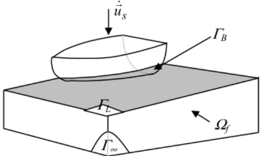
Figure 1. Geometrical definitions

We consider the problem of the impact of a three-dimensional body on a free surface (Fig. 1). The water entry problem is expressed within the framework of potential flow theory. Indeed, the fluid is assumed to be perfect and incompressible and the flow is irrotational. The velocity field can therefore be evaluated according to v=gradφ, where

) t , z , y , x ( φ =

φ is the velocity potential. Under these assumptions, the velocity potential must satisfy an elliptic problem with a body boundary condition that expresses the continuity of the normal velocity component on the fluid-structure interface. The kinematic and dynamic free surface conditions, respectively, state that the free surface is a material surface along which the pressure is constant. Moreover, the fluid is assumed to be initially at rest. Finally, the problem to be solved in velocity potential formulation is

0 = φ ∆ in Ωf (1) n . u n s r &r = ∂ φ ∂ _{on the body} ₍₂₎ 0 gz p ) grad ( 2 1 t 2 ₊ ₌ ρ + φ + ∂ φ

∂ _{on the free surface} ₍₃₎

0 z h grad . grad t h = ∂ φ ∂ − φ + ∂

∂ _{on the free surface} ₍₄₎

where ur_s(x,y,t) is displacement of the body and h is the free surface elevation. The structural equations will be presented after.

Such a problem remains difficult to solve directly because of the unsteady non-linear boundary values and the free surface presents violent motions that are expressed experimentally by a jets developing along the body (see Greenhow 1987).

According to Wagner, the problem is classically written on the plan z=0 on which the boundary conditions are projected. ΓB and ΓL are respectively the projection of the wetted body surface and the free surface. The contact line _Γ(t),

defined as the intersection between ΓB and ΓL is unknown a priori.

The problem requires the gravity effect and quadratic terms to remain small compared to the linear terms. Physically, the acceleration of the fluid has been assumed to be larger compared to gravity which can be neglected for the impact problem. The displacements of the body and the free surface must also remain small to justify the geometrical linearization of the boundary conditions. Cointe (1989) and Wilson (1989) have justified the linearization through an asymptotic analysis of the impact problem for a blunt and rigid body by introducing a small parameter. This one represents the ratio between the immersion and characteristic length scale of the wetted body area.

Using matched asymptotic expansions method entails to define two zones in which two asymptotic expansions are performed and matched successively:

! The far field domain, where the flow is similar to the one around a flat plate of unknown width in an unbounded fluid,

! The spray root domain near the contact line, were the flow over turns to create a jet.

It is worth noting that a third asymptotic expansion can be performed in the jet domain, along the body, but the contribution of this solution can be neglected in the leading order.

The perturbation procedure relies strongly on the blunt body assumption. In the far field, the body boundary condition can be written on the undisturbed position without introducing significant error. The exact dynamic condition is replaced on neglecting the quadratic terms for the leading order by a Dirichlet condition for the free surface. These quadratic terms have to be retained for the second asymptotic expansion to describe the flow within the jet.

The simplified kinematic free surface condition states that the vertical displacement of the free surface is equal to the fluid vertical motion, evaluated on the linearised position of the free surface.

Finally, the hydrodynamic problem, linearised with an asymptotic approach is written as

0 = φ ∆ in Ωf, (5) n . u n s r &r = ∂ φ ∂ _on_Γ B, (6) 0 = φ on ΓL, (7) z t h ∂ φ ∂ = ∂ ∂ _on_Γ L. (8)

The pressure is given by the Lagrange linearized equation, t p ∂ φ ∂ ρ − = (9) ΓB Γ∞ ΓL Ωf s u&r

(4)

In order to describe the structure, the usual small perturbations assumption is made, and the equilibrium equation reads f v i d us d r r &&r ₌ _Σ₊ ρ in _Ωs, (10)

where Σ denotes the stress tensor, ur corresponds to thes

structural displacement, and f corresponds to volume force associated for example with the gravity field. If gravity effects do not contribute to the local deformations here, they nevertheless influence the global motion of the body before impact. The boundary condition on the structure is

n . n . s f r Σ= r Σ on ΓB, (11)

where the subscripts f and s respectively refer to the fluid and

the structure.

The structural modeling is performed within the framework of linear elasticity. Hooke’s law is used to express the relation between the stresses and the strains which are given by the linearized Green-Lagrange tensor ε ,

(

i,j ji,

)

ij u u 2 1 + = ε (12)

2.2 Determination of the wetted surface

As mentioned previously, the wetted portion of the body is unknown. The contact line is determined by the volume of fluid conservation (Wilson 1989, Fontaine & Cointe 1992) which is satisfied by the Laplace's equation. In order to find this line, it is easier to introduce a displacement potential, as suggested by Korobkin (1982), given by

∫

φ = ψ t 0 (x,y,z;s )ds ) t ; z , y , x ( (13)

The problem to solve in the displacement potential is the same Neumann-Dirichlet boundary conditions problem as for the velocity potential. The wetted surface is determined through an iterative procedure. Starting from an initial surface guess for (ΓB)0, the problem for displacement potential

problem is solved until that the free surface elevation is equal to the position of the body at the boundary Γ(t)

z . u t) y, h(x, =rs r. (14)

Once convergence has been reached, the position of the contact line is known. The linear system for the velocity potential is then solved.

2.3 Numerical resolution

The problem is solved using the Finite Element Method, for the fluid as well as the structure, based on a variational formulation. We have considered the weighting function ϕ for the fluid, which verifies the boundary condition ϕ = 0 on ΓL and U* for the structure kinematically acceptable to 0.

Galerkin’s method is used to approximate the different functionsφ, ϕ, U and U*,

{ }

e f N > ϕ =< ϕ , (15)

{ }

e f N > φ =< φ , (16)

[ ]

{ }

e s s N U u = , (17)

[ ]

{ }

e s s* N U* u = , (18)

where the shape functions N… depend on the types of elements, and the vector {…}e_{denotes the nodal unknown} vector of the finite element (e). The problem after discretization, takes the following form,

[ ]

H

{ }

φ =

[ ]

FS

{ }

U& , (19)

[ ]

{ }

&& +

[ ]

{ }

=−

[ ]

T

{ }

φ& f s U K U ρ FS M , (20)

{ }

[ ]

∫

= e B Γ s T f e _{N _}_n _N _dS [FS] , ₍₂₁₎

where the mass and stiffness matrix, respectively [Ms] and [K], and the matrix [H], are obtained by assembly of the elementary terms calculated on each finite element (e). The terms

[ ]

FS &

{ }

U represent the continuity of the normal velocity on the wetted surface of the body and −

_{[ ]}

T

{ }

φ&

f FS

ρ , the

contribution of the pressure on the same surface _ΓB, pressure given by the equation (9). So the pressure imposed by the fluid drives the structural deformations and the structural deformations influence the pressure field through the body boundary condition In order to obtain a robust method to solve the coupled fluid – structure interaction problem, all the evolution equations are integrated simultaneously. The structural deformations are included in the fluid flow discrete formulation, while the pressure is expressed as the time derivative of the velocity potential in the discrete structural analysis.

This model is not sufficient to describe the fluid because of the pressure distribution, which is singular close to the boundary wetted surface. This singularity is due to the linearization. It is necessary to correct this pressure with the solution obtained in the spray root domaine.

The numerical resolution of the problem is performed using the commercial Finite Element Method code Castem. An external procedure is implemented for the evaluation of

(5)

the coupling matrix [FS]. The correct implementation of the approach has been checked for the test case problem of sloshing in a rectangular tank including an elastic beam in its center for two-dimensional case (Tourbier et al. 2002). This problem has been studied experimentally by Chaï (Chaï, 1996). For the three-dimensional case, it has been checked for a plate surrounded by water.

The fluid–structure interaction problem is then integrated starting from the initial conditions in a numerical temporal explicit or implicit scheme with a time step dt. Nevertheless, studying for rigid body slamming, it appears that time step dt

for the fluid problem has to be less than the fiftieth part of the instant to calculate accurately pressure distribution. Choosing the same time step for the coupled problem simulation leads to generate a high costly time procedure. Consequently, we solved the fluid-structure interaction problem with an iterative procedure. The fluid problem is first solved with a step time

δt. After determination of the force due to the pressure, the structural resolution is within the Newmark temporal integrated sheme with the step time _∆t. The time schema is represented by Figure 2 :

Figure 2. Resolution schema applied to solve the coupled problem

3 VALIDATION OF THE NUMERICAL PROCEDURE Comparisons for a paraboloid elliptic shaped hull are presented in Figure 3. Hexahedron types of elements were used in the numerical simulation. Good agreement has been noted between numerical simulations and analytical results of

the wetted surface for a rigid body. The free surface is well described by the displacement potential.

Figure 3. Free surface elevation during impact of paraboloïd elliptic

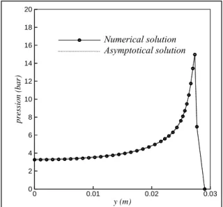
Next, we present results for rigid wedge penetrating with a constant velocity V a free surface initially at rest. The numerical method previously described has been applied to this case. Comparisons between numerical and analytical pressure results are presented in figure 4. Triangular and quadrilateral elements were used for the numerical computation. Figure 5 illustrates the importance of including the inner solution which describes the formation of a jet. The analytical pressure distribution is matched to the numerical solution.

Figure 4. Pressure distribution for the impact of a wedge

To conclude this section, analytical and numerical results are very close to each others for both 2D and 3D cases, which validate the numerical approach. The evaluation of the free surface elevation remains nevertheless sensitive to the boundary between the structure and the fluid. To represent the ∆t t n+1 p {u} ] FS [ } [H]{ψ = tn p } u { ] FS [ } [H]{φ = & 2_δt {u } p = {u } n+ 1 {u } p = {u } n+ 1

Calculation of the pressure force

Structure resolution (implicit) Fluid resolution 1 n 1 n _{_F_} {u} ] K [ + ₌ + t 2 } { } { ] FS [ } {F T n1 t n1 t f 1 n δ φ − φ ρ − = ++δ +−δ + small axis wide axis 0 0.01 0.02 0.03 y (m) 0 2 4 6 8 10 12 14 16 18 20 p re ss io n (b a r) pcompositeMEF pcompositeasympt. Numerical solution Asymptotical solution

(6)

singular behavior of the solution in the vicinity of this boundary, the finite elements mesh has to be refined in this zone. The regularity of the mesh is also an important parameter, which controls the accuracy of the numerical resolution.

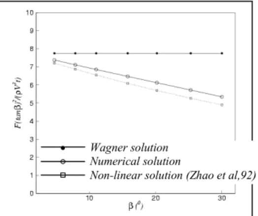
Figure 5. Force evolution versus deadrise angle of wedge. Comparison between outer solution (Wagner), corrected

numerical solution (MEF) and non-linear solution 4 EXPERIMENTS

In this part, we present investigation tests the objective of which are to provide some experimental results to validate the previous numerical approach. We first describe the experimental test carried out at the Mechanical and Material Laboratory (Donguy, 2002). Then experimental results on rigid and deformable structures are presented and finally comparisons with the numerical results are carried out.

4.1 Experimental set-up

The investigation tests consist of free fall drop test of cone shaped model. Drop test with impact velocities varying from 2m/s to 8 m/s are realized from free falling rig system (see Figure 6) of 3.5 m height. The cone fell in a water tank of 1 m deep and 1.20 m diameter. A foam is on the bottom to progressively stop the cone.

Cones shaped models were rigidly attached to a cylindrical support of 322 mm diameter (see Figure 7). Three different cone shaped models with deadrise angles of 6, 10, and 14 degrees have been successively tested. To study the deformation influence, rigid body and elastic structure are tested. The effective thickness of the steel models were sufficiently important, reaching from 25 to 50 mm, so that the rigid body assumption is verified during impact. For elastic structure three thickness have been chosen equal to 0.5 mm – 1 mm – 1.5 mm.

The use of a relatively large experimental facility allows for a typical size of 0.32 m for the tested models, therefore reducing

the possible influence of surface tension effects. The impact velocity was chosen to increase by realistic values from approximately 2 to 6 m/s.

Figure 6. Impact tower: experimental set-up

Figure 7. Detailed views of the cone shaped models with different deadrise angles

Velocity cable sensor Winch Cone Rig Water tank Foam e = 29 _{φ 322} 90 40 Rigid cone Cylindrical support e = 16 Additional mass Wagner solution Numerical solution

(7)

Drop velocity and pressure measurements were performed during impact. Two quartz ICP compensated pressures sensors were set at 40 mm and 90 mm from the cone symmetry axis (fig. 8). These sensors are well suited for impact measurements. Their sampling frequency is up to 400 kHz, and the measurement range is 0 to 69 bar. They also allow for the use of relatively long wires (20 m) without altering the electric signal so that the data processing system does not need to be too close to the water.

The drop velocity was measured by mean of a cable sensor connected to the cylindrical support. Finally, pressure and velocity signals were plotted and recorded by a numerical memory oscilloscope. The cones were dropped against calm water. At least three drops were performed in each test condition to make sure of the repeatability of the measurements. Results presented below are representative of these drop test series.

4.2 Signal on the rigid body

Figure 8. Pressure and velocity evolution during impact of the 10° rigid cone – Vimpact = 2.5 m/s

Figure 9. Correspondence between pressure history and cone location

Figure 8 represents historical evolutions of the pressure on the two sensors p1, p2 and the velocity during the impact for

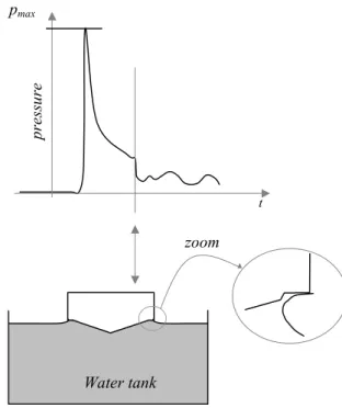
10° deadrise angle cone and for an impact velocity of 2.5 m/s. For other velocities and cone characteristics, the evolutions are equivalent. Firstly, we controlled that the global velocity impact is constant during the water entry. The small perturbation on the signal is due to the mean of velocity measuring by cable sensor. We noticed a similar evolution of the measured pressure on both sensors. First, we observed a slight depression which comes before the pressure peak. The explanation of this depression is due to the separation of the jet and then to the creation of in–draught. Then, the pressure peaks are reached when the sensors are in the jet formation and more precisely at the stagnation point. The rise velocity of the pressure depends of the velocity impact and the conicity. It is 10 µs for the fastest and 200 µs for the slowest. After the peak pressure, we noted a slow decrease of the pressure in the meantime that the cone is progressing in the water. This is in accordance with the fact that the sensor goes away the free surface. Finally, a sudden decrease of the pressure happens simultaneously on the two sensors. At this instant, the jet zone is on the cylindrical support and the cone is then wholly in the water. There is separation of the jet in the air so that the pressure decreases suddenly on the cone. A blowup of a segment of figure 10 schemes this situation.

Figure 10. Correspondence between the sudden pressure decrease and the cone position in the water

t pre ssu re pmax zoom Water tank

Free surface at rest

III

II I

(8)

4.3 Signal on the elastic structure

For the test realized on the rigid body, the measured signal Figure 8 is representative of the whole measurement made for all the cone-shaped models. The test performed on the elastic structure presents more disparity. In particular, some phenomena not very perceptible in the case of rigid body become more important and new phenomena appear and bring to the fore the influence of structural deformation

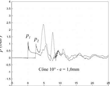
First, the phenomenom of depression becomes widely more important. And, as we can notice from Figure 11 this phenomenon can become enough important to influence the intensity of the value of the second pressure peak. New phenomena occur on all shaped models: this is an apparition of a second pressure peak. This peak of pressure is due to the geometrical configuration of the cylindrical support which presents a flat circumference. Due to the fact that the maximum value of the pressure varies versus the slope of the structure surface and more precisely is higher for small deadrise angle, it seems that when the jet formation is on the flat part of the cylindrical support, the pressure rises suddenly on the entire cone surface and creates the second peak pressure. Then this is the geometry configuration body which generates the second peak.

Figure 11. Pressure and velocity evolution during impact of the 10° deformable cone (e=1 mm)

Vimpact = 2.5 m/s

4.4 Comparisons between theory and experiments Table 1 reports the two maximum values of the pressure on sensors p1, p2 measured and calculated, for the three

deadrise angles (β). Numerical and experimental results for the pressure levels are found to be in reasonable agreement although the pressure is always slightly over predicted, indicating that the numerical model is therefore conservative.

Vimpact = 2.5 m/s Exp. Num.

Cone 6° 2.8 2.7 4.6

Cone 10° 1 1.4 1.6

Cone 14° 0.7 0.7 0.8

Vimpact = 5.2 m/s Exp. Num.

Cone 6° 10.3 10.7 19.8

Cone 10° 3.9 5.5 7

Cone 14° 2.6 2.7 3.5 Table 1. Comparison between predicted and experimental peak pressure value for different impact

velocity of the rigid cone

On the first sensor the experimental value is by far over predicted for all deadrise angles but less for the 14° cone than the 6°. Difference is less pronounced for experimental values on the second sensor. Decay of the pressure can be explained physically by air entrapment. This phenomenon has also been observed by Chuang (1971) on cones with deadrise angles smaller than 1°, and by Hagiwara & Yuhara (1974) for wedges with deadrise angles lower than 3 degrees.

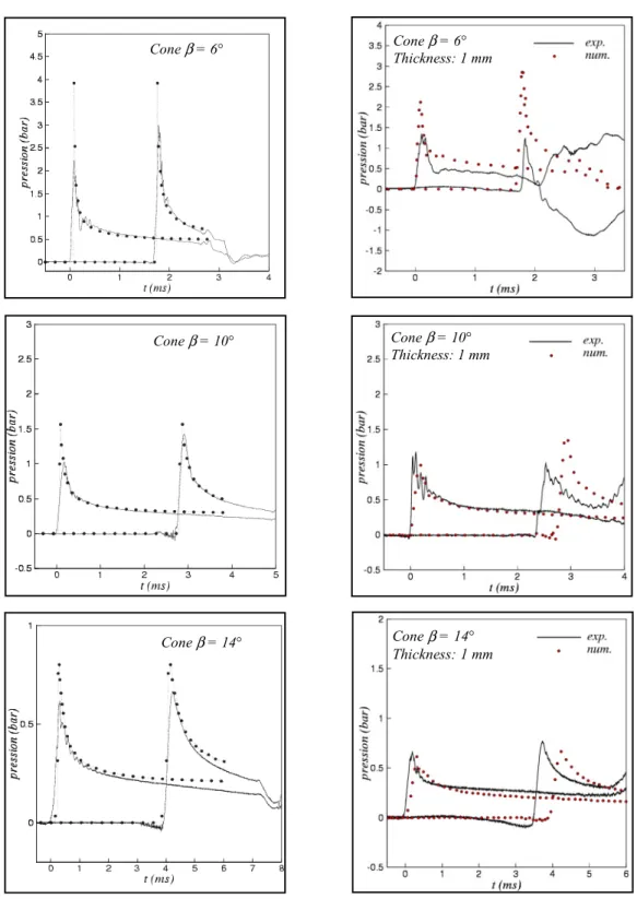
Examples of temporal evolution of the pressure on the two probes are presented in Figure 12 (a) (b) (c) corresponding to the different deadrise angles and impact for rigid body. The experimental distribution is globally well represented by the numerical simulation. Both signals show a pressure peak travelling along the body, followed by a plateau. The location of the peak is clearly well described by the simplified theory. The wetted length seems therefore to be correctly estimated. This local quantity results nevertheless from global volume conservation property as mentioned previously. It is therefore not surprising that the modeling is able to give a good estimate of this quantity. The pressure rise immediately after impact is also well reproduced. The simplified model is indeed asymptotically valid for small times. The level of the peak, i.e., the maximum pressure, is reasonably estimated for the biggest deadrise angle, but the error increases with a decrease of the deadrise angle. According to the asymptotic solution, the level of the pressure peak should not vary along the body. The experiments clearly indicate that the peak intensity increases between the two probes. This discrepancy can be partially explained by air entrapment phenomenon. This phenomenon is not reproduced in the numerical simulation where the impact velocity remains constant.

As well as for the description of the pressure distribution on elastic structure, comparisons between numerical and experimental results are more difficult. On one hand, the depression zone can’t be reproduced numerically because the air entrapment phenomenon hasn’t been taken into account. Cône 10° - e = 1,0mm

(9)

On the other hand due to the fact that the second peak zone comes from the geometrical configuration of the cone and occurs after the period of time we interested in, we haven’t reproduced it. So, the major difference between numerical results and an experimental test comes from the velocity of the peak progression. Indeed we noticed the instant at which the peak pressure occured is different from experimental to numerical case. In spite of this dissimilitude, the global numerical pressure distribution fits well. We remarked moreover the comparison is better for the bigger conicity than the smaller for which the water perturbation are more significatve.

5 CONCLUSION

In the present paper, the three-dimensional slamming problem has been studied. After having presented the governing equation for the coupled problem, relying on asymptotic theory in velocity potential and small perturbations. Experimental investigations have been studied. It consisted in free fall drop-tests of deformable cone shaped models. Each cone presented different deadrise angles and thickness. The numerical results have been well confirmed by experimental ones.

All this study takes place within the asymptotic theory, entailing the boundary conditions projection. In order to avoid this assumption, we can used the ALE (Arbitrary Lagrangian Eulerian) or X-FEM (extended Finite Element Method) that are a priori able to follow the evolution of a free surface. 6 REFERENCES

Armand, J.L, Cointe, R. (1986) “Hydrodynamic impact

analysis of a cylinder”, 15th OMAE/ASME symposium,

vol.1, pp.250-255.

Chai, X.J. (1996) “Influence de la gravité sur les interactions fluide-structure pour un fluide dans un domaine borné à

surface libre”, Thesis, Institut National Polytechnique de

Lorraine.

Cointe, R., Armand, J.L. (1987) “Hydrodynamic impact analysis of a cylinder” J. Offshore Mechanics and Artic

Engineering, vol. 9, pp. 237-243.

Cointe, R. (1989) “Two dimensional water solid impact”

Journal of Offshore Mechanics and Arctic Engineering,

vol.111, pp.109-114.

Chuang, S.L., Milne, D.T. (1971) “Drops test of cones to investigate the three-dimensional effects of slamming” Navy Naval Ship Research and Development Center, Report 3543.

Donguy, B., Peseux, B., Fontaine, E. (2000) “On the ship structural response due to slamming loads ” Proc. of European Congress on Computational Methods in Applied Sciences and

Engineering, Barcelona.

Donguy, B. (2002) “Etude de l’intéraction fluide-structure lors de l’impact hydrodynamique”,Thèse, Ecole Centrale de Nantes.

Faltinsen, O. (1997) “The effects of hydroelasticity on ship slamming” Phil. Trans. R. Soc. Lond., vol. 355, pp. 575-591. Fontaine, E., Cointe (1997) “Asymtotic theory of water entry”,

High Speed Body Motion in Water, Kiev, NATO Conference.

Greenhow, M. (1987) “Wedge entry into initially calm water”

Applied Ocean Research, vol. 9, pp. 214-223.

Fontaine, E., Cointe, R. (1992) “A second-order solution for

the wedge entry with small deadrise angle”, Seventh

International Workshop on Water Waves and Floating Bodies, Val de Reuil.

Hagiwara, K., Yuhara T. (1974) “Fundamental study of wave impact loads on ship bow” Journal of the Society of Naval

Architect vol. 135

Howison, S.D., Ockendon, J.R., Wilson S.K. (1991) “Incompressible water entry problems at small deadrise angles” Journal of Fluid Mechanics, vol. 222, pp. 215-230 Korobkin, A.A. (1982) “Formulation of penetration problem as a variational inequality” Din. Sploshnoi Sredy, vol. 58, pp. 73-79

Korobkin, A.A. (1995) “Wave impact on the bow end of a catamaran wetdeck” Journal of Ship Research, vol. 39, pp. 321-327.

Magee, A,, Fontaine, E. (1998) “A coupled approach for the evaluation of slamming loads on ships” Proc. 7th_{Int. Symp. on}

Practical Design of Ships and Mobil Units, The Hague

Netherlands.

Scolan, Y.M., Korobkin, A.A. (2001) “Three-dimensional theory of water impact. Part 1. Inverse Wagner problem”,

Journal of Fluid Mechanics, vol 440, pp 293-326.

Tourbier, M., Donguy, B., Peseux, B., Gornet, L. (2002) “Modelization and simulation of the three-dimensional hydrodynamic impact problem” Proc. of Pressure Vessels and

Piping ASME Conference, Vancouver.

Wagner, H. (1932) “Über Stoss und Gleitvorgänge an der Oberfläche von Flüssigkeiten” Z. Ang. Math. Mech., vol. 12, pp. 193-215.

Von Karman, T. (1929) “The impact on a sea plane floats during landing”, Technical Notes for National Advisory Comittee for Aeronautics.

Wilson, S.K. (1989) “The mathematics of ship slamming”

Ph.D. thesis, University of Oxford.

Zhao, R., Faltinsen, O.M., Aarsnes, J.V. (1996) “Water entry of arbitrary two-dimensional sections with and without flow separation” Proc. 21st_{Symposium on Naval Hydrodynamic}_, Trondheim, Norway.

(10)

e

Figure 12. Pressure histories - Comparison between numerical (straight line) and experimental (dot line) results for rigid cone (at left) and for deformable structure (at right)

Cone _β = 10° Cone _β = 14° Cone β = 6° Cone β = 14° Thickness: 1 mm Cone _β = 10° Thickness: 1 mm Cone _β = 6° Thickness: 1 mm