HAL Id: hal-02377711
https://hal.archives-ouvertes.fr/hal-02377711
Submitted on 8 Dec 2020HAL is a multi-disciplinary open access archive for the deposit and dissemination of sci-entific research documents, whether they are pub-lished or not. The documents may come from teaching and research institutions in France or abroad, or from public or private research centers.
L’archive ouverte pluridisciplinaire HAL, est destinée au dépôt et à la diffusion de documents scientifiques de niveau recherche, publiés ou non, émanant des établissements d’enseignement et de recherche français ou étrangers, des laboratoires publics ou privés.
Effect of Cloud Cover on Temporal Upscaling of
Instantaneous Evapotranspiration
Yazhen Jiang, Xiao-Guang Jiang, Ronglin Tang, Zhao-Liang Li, Yuze Zhang,
Zhao-Xia Liu, Cheng Huang
To cite this version:
Yazhen Jiang, Xiao-Guang Jiang, Ronglin Tang, Zhao-Liang Li, Yuze Zhang, et al.. Effect of Cloud Cover on Temporal Upscaling of Instantaneous Evapotranspiration. Journal of Hydrologic Engi-neering, American Society of Civil Engineers, 2018, 23 (4), pp.05018002. �10.1061/(ASCE)HE.1943-5584.0001635�. �hal-02377711�
Effect of Cloud Cover on Temporal Upscaling of
1
Instantaneous Evapotranspiration
2
Yazhen Jiang 1, Xiao-guang Jiang 2, Ronglin Tang 3,*, Zhao-Liang Li 4, 3
Yuze Zhang 5, Zhao-xia Liu 6, Cheng Huang 7 4
1. University of Chinese Academy of Sciences, Beijing 100049, China; 5
E-mail: jiangyazhen15@mails.ucas.ac.cn; 6
2. University of Chinese Academy of Sciences, Beijing 100049, China; State Key Laboratory of 7
Resources and Environmental Information System Institute of Geographic Sciences and Natural 8
Resources Research, Chinese Academy of Sciences, Beijing 100101, China; Key Laboratory of 9
Quantitative Remote Sensing Information Technology, Academy of Opto-Electronics, Chinese 10
Academy of Sciences, Beijing 100094, China. 11
3. State Key Laboratory of Resources and Environmental Information System Institute of Geographic 12
Sciences and Natural Resources Research, Chinese Academy of Sciences, Beijing 100101, China; 13
University of Chinese Academy of Sciences, Beijing 100049, China. 14
4. Key Laboratory of Agri-informatics, Ministry of Agriculture/Institute of Agricultural Resources and 15
Regional Planning, Chinese Academy of Agricultural Sciences, Beijing 100081, China; Icube 16
(UMR7357), UdS, CNRS, 300 Bld Sébastien Brant, CS10413, Illkirch 67412, France. 17
5. University of Chinese Academy of Sciences, Beijing 100049, China. 18
6. Xinjiang Institute of Ecology and Geography, Chinese Academy of Sciences, Urumchi 830011, 19
Xinjiang, China. 20
7. University of Chinese Academy of Sciences, Beijing 100049, China. 21
* Correspondence: tangrl@lreis.ac.cn; Tel.: +86-10-6488-8172 22
23
2
Abstract: Studying the effect of cloud cover on temporal upscaling of instantaneous
24
evapotranspiration (ET) is significant in efforts toward a more accurate and widely applied
25
upscaling method to obtain exact ET at daily or longer time scale, thereby benefiting
26
practical applications. In this article, the authors concentrated on the effects of cloud cover
27
with different amounts and time durations on three commonly used upscaling approaches
28
including the constant evaporative fraction (EF) method, the constant reference evaporative
29
fraction (EFr) and the constant global solar radiation (Rg) method. Transient cloud and
30
persistent cloud were both defined according to occurrence time, namely, cloud appearance
31
one hour before or after the upscaling moment and the cloud lasting the whole daytime
32
except during upscaling time, respectively. Different cloud cover amounts were indicated
33
by different losses of downwelling shortwave irradiance. Instantaneous fluxes were
34
simulated from the Atmosphere-Land-Exchange (ALEX) model, which is driven by
35
meteorology measurements at the Yucheng station. The results show that: (I) the cloud will
36
deteriorate with the underestimation or overestimation of daily ET upscaling compared to
37
the results of clear days. Specifically, persistent cloud had a more significant effect on the
38
three upscaling methods; for transient cloud, the upscaling results had larger deviations
39
when the cloud appeared before the upscaling moments than when it appeared after; (II) the
40
effect on the upscaling factors and upscaling results both increased proportionally with the
41
growth of cloud cover; (III) the constant EFr method performed best for both clear and
42
cloudy situations with a minimal bias, less than 4.7 W/m2 (5.5 %) and an RMSE less than
43
8.9 W/m2 (20.6 %); the EF method was most severely affected with a bias up to 24.1 W/m2
44
(28.3 %)and an RMSE up to 24.9 W/m2 (57.7 %); the Rg method had intermediate accuracy
45
with a bias less than 20.9 W/m2 (24.6 %) and an RMSE less than 20.3 W/m2 (47.1 %); (IV)
46
all three approaches were influenced more significantly near noontime.
Keywords: Temporal upscaling; Cloud cover effect; Evapotranspiration; Fluxes simulation
48
1. Introduction
49
Evapotranspiration (ET) can be used effectively to express vegetation water
50
consumption and surface moisture. Routine monitoring of actual ET is widely considered a
51
significant scientific issue benefiting practical applications in a variety of fields, including
52
water management, water rights regulation, drought monitoring and the study of climate
53
change (Li et al., 2009; Tang et al., 2011; Cammalleri et al., 2014). Remote-sensing based
54
approaches can be used to estimate the spatial distribution of ET at the regional or basin
55
scale when satellite data are available (Courault et al., 2005), overcoming the problem
56
related to conventional methods that they are being applied only at the site or field scale.
57
However, current remote-sensing based ET models generally only provide snapshots of ET
58
at the time of satellite overpass (Gómez et al., 2005; Colaizzi et al., 2006. Chávez et al.,
59
2008), and ET integration over a longer time scale (days, months to years) is more important
60
among many applications. Therefore, the instantaneous ET values at satellite overpass time
61
must be upscaled temporally to make more sense.
62
Various ET temporal upscaling methods have been developed by assuming
63
self-preservation of the ratio between ET and a given reference variable over the daytime
64
hours (Crago, 1996; Bastiaanssen, 2000; Delogu et al., 2012). The constant evaporative
65
fraction (EF) method is one of the most commonly used upscaling approaches, which
66
assumes that EF (the ratio of latent heat flux to available energy) is constant during the
67
daytime (Shuttleworth, 1989). Daily ET in this method can be obtained with daily available
68
energy (difference of net radiation and soil heat flux) and remotely sensed instantaneous EF.
69
A variety of studies have demonstrated the constancy of EF and its effectiveness in upscaling
70
instantaneous ET from remote sensing data in clear skies (Nichols and Cuenca, 1993;
71
Gentine et al., 2007). In the application of this method, the daytime ET is usually
4
underestimated by 5%–10% (Brutsaert and Sugita, 1992; Chávez et al., 2008), which is
73
partly due to the EF curve usually exhibiting a concave shape under wet conditions and the
74
instantaneous EF near the noon is lower than the daily averaged value (Lhomme & Elguero,
75
1999; Hoedjes et al., 2008). The underestimation is corrected by directly adding 10% ET in
76
some studies (Anderson et al., 1997). Despite the controversies raised regarding its validity,
77
the EF conservation method has been widely applied (Gómez et al., 2005; Galleguillos et al.,
78
2011; Delogu et al., 2012).
79
Trezza (2002) introduced another ET upscaling method using standardized reference
80
evapotranspiration (ETr) as the variable that depicts the diurnal variations of net radiation, air
81
temperature, wind speed and relative humidity. This method is the so-called constant
82
reference evaporative fraction (EFr, the ratio of actual ET to ETr) method (Allen et al., 1998;
83
2006). The EFr is assumed to be constant during the daytime, and daily ET can be estimated
84
through the ratio, together with daily ETr. In this upscaling method, a fixed surface
85
resistance is usually used for the calculation of ETr. Tang et al. (2017 a) haveinvestigated
86
the application of variable surface resistances from the Penman-Monteith (PM) equation and
87
found the accuracy could be improved only in some upscaling moments.Previous studies
88
have stated that maintaining the conservation of EFr in a diurnal cycle could provide better
89
estimates of daily ET under advective conditions (Trezza, 2002; Allen et al., 2007).
90
Other widely employed upscaling methods assume that the ratios between latent heat
91
flux and other variables (e.g., solar radiation, solar radiation irradiance) are constant during
92
the daytime, during which the variables are generally the primary energy drivers of surface
93
water and energy transfer. For instance, latent heat flux and solar radiation are reported to
94
have similar diurnal variations (e.g., sine functions), and the method mentioned is the
95
constant global solar radiation (Rg) method. Daily ET values have already been estimated
96
with this relationship (Zhang and Lemeur, 1995; Ryu et al., 2012; Niel et al., 2011). Ryu et al.
(2012) adopted the constant Rg method to upscale the remotely sensed ET to daily and
98
eight-day averaged values and showed it was a robust scaling method.
99
It appears that almost all of these upscaling methods can be effectively used to acquire
100
daily ET over clear-sky days (Brutsaert and Sugita, 1992; Colaizzi et al., 2006; Ryu et al.,
101
2012). The issue that arises is that cloud coverage is a prominent phenomenon in many
102
parts of the world, and the mean cloud cover per day may even exceed 60% in the humid
103
tropics (Bussieres and Goita, 1997). Cloud covers usually cause reductions in solar radiance
104
and available energy, and thus affect diurnal changes in ET. Different occurrence times,
105
coverage amounts and durations of cloud will have markedly different effects on ET
106
variation, which will further influence applications of these upscaling methods that assume
107
some self-preservative ratios between ET and other variables (Suigita and Brutsaert, 1991;
108
Zhang and Lemeur, 1995; Crago, 1996). Jackson (1983) noted that the amount and duration
109
of cloud cover during the daytime will affect the accuracy of upscaling methods. Niel and
110
Mcvicar (2012) also indicated that the assumption of clear sky conditions during the whole
111
day is not always assured for remote sensing applications, and it is feasible that only the
112
specific time of the satellite overpass must be clear. To the best of our knowledge, the
113
studies of these method as they relate to the effective assessment of cloud coverage are very
114
rare, and ET was obtained in some applications from satellite images for a succession of clear
115
days and interpolating the ratios for cloudy ones (Carlson et al., 1995; Xu et al., 2015). The
116
presence of clouds is linked to a decrease in irradiance at the surface, and the cloudy days
117
indicated by irradiance reduction have been validated as heavily overcast days using
118
measurements. In Long’s study (2000; 2006), cloud was defined as the difference between
119
the measured downwelling irradiance and that expected for clear-sky conditions. Therefore,
120
an elaborate understanding of the cloud cover effect on upscaling procedures is imperative
121
and feasible.
6
The objective of this paper is to comprehensively evaluate the cloud effect with
123
different occurrence times, coverage amounts and duration times on these three temporal
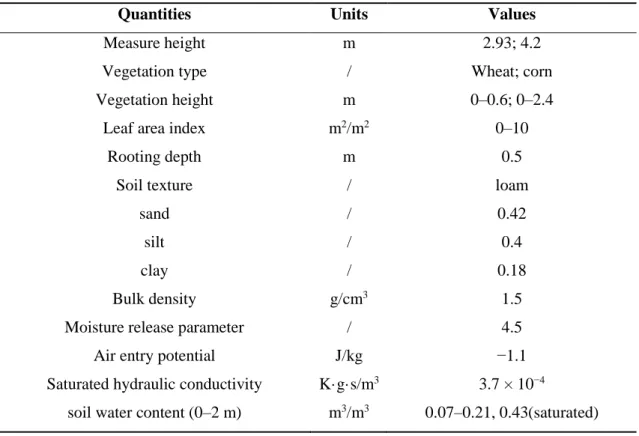
124
upscaling methods to explore an upscaling approach that can effectively consider the cloud
125
effect and obtain exact daily ET. Instantaneous ET are simulated from the
126
Atmosphere-Land-Exchange (ALEX) model. Transient cloud (cloud occurred one hour
127
before or after the upscaling time, respectively) and persistent cloud (cloud lasted for almost
128
the whole daytime except the upscaling time) were defined according to diverse appearance
129
and duration time. Different cloud cover amounts were represented by the reduction of
130
downwelling short wave irradiance of clear skies. The ratios between the ET and other
131
variables, regarded as upscaling factors, are all assumed to be self-preservative in these three
132
upscaling methods. The specific work of this current paper is to: (i) estimate the effect of
133
different clouds on upscaling factors, (ii) estimate the effect of different clouds on upscaling
134
results obtained through different upscaling methods compared to that of clear days, and (iii)
135
find upscaling methods that have stable performances even under cloudy conditions.
136
2. Study area and data
137
2.1 Study area 138
This study was carried out at Yucheng station(36.8291º N, 116.5703º E), which is in
139
southwestern of Yucheng County, Shandong Province, in North China (Figure 1). The
140
Yucheng station is part of the Chinese terrestrial ecosystem flux network, which aims to
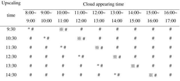
141
measure the long-term exchange of carbon dioxide, water vapor, and heat between the land
142
and the atmosphere. The climate is subhumid and monsoonal, with a mean annual
143
temperature of 13.1℃ and precipitation of 528 mm. The soil is sandy loam, and the land
144
cover types near the station primarily consist of crop (winter-wheat and summer-corn
145
rotation), bare soil, trees and water.
2.2 Study data 147
The measurements from Yucheng station used in this study contain meteorological
148
variables, radiation data, flux data and MODIS data for the period from late April 2009 to late
149
October 2010. This period covers two phenological stages from emergence to close-to-peak
150
biomass in winter wheat and summer corn. Meteorological variables, including air
151
temperature, wind speed, relative humidity and atmospheric pressure, were measured at the
152
height of 2.93 m during the growth period of wheat and at 4.2 m during the growth period of
153
corn. Radiation data, including downwelling and upwelling shortwave and longwave
154
radiations, were acquired from a CNR-1 radiometer installed at the height of 3.98 m. The
155
sensible heat flux (H) and latent heat flux (LE) were measured by an Eddy Covariance (EC)
156
system consisting of an open-path CO2/H2O gas analyzer and a 3-D sonic
157
anemometer/thermometer. The height of the EC facility was 2.7 m and 3.75 m during the
158
growth period of wheat and corn, respectively.Soil heat flux (G) was estimated from a single
159
HFP-01 soil heat flux plate at 2 cm below the surface without considering heat transfer for
160
the 2 cm storage layer above the plate. MODIS cloud quality control product (MOD35) was
161
downloaded from the Atmosphere Archive and Distribution System Web
162
(https://ladsweb.nascom.nasa.gov/data/search.html).
163
All the meteorological variables and the EC measurements were made in an
164
experimental area with dimensions of approximately 250 m by 90 m at Yucheng station. The
165
crop type of the experimental area is relatively uniform during the measuring periods. All
166
data are recorded as a 30-min average, and there are 48 records in a day for each variable.
167
Meteorological variables averaged every half hour and radiation data were collected as input
168
data to drive the ALEX model. The in situ fluxes are used to validate the simulated results. It
169
is noted that five-minute averaged data of downwelling shortwave radiations and MOD35
170
are also obtained for clear sky identification.
8
3. Methodology
172
3.1 ET upscaling method 173
In this study, as described above, the upscaling methodologies for extrapolating
174
instantaneous ET to daily value tested were the EF method, the EFr method and the Rg
175
method, respectively. Three upscaling methods were performed to estimate the actual daily
176
ET from a single time-of-day snapshot, by assuming conservation of some ET factors over
177
the course of the day. These factors are generally expressed as ratios between instantaneous
178
ET at a specific time and a reference variable that can be computed hourly.
179
In the EF method, the EF factor was the ratio of latent heat flux (LE, used
180
interchangeably with ET in this paper) to surface available energy (surface net radiation
181
minus soil heat flux), expressed as
182 ( ) ( ) ( ) ( ) i d i d n i d LE EF R G (1) 183
The subscripts “i” and “d” represent the instantaneous and daily averaged values,
184
respectively. The daily LE can be estimated once the daily integrated net radiation Rn and the
185
instantaneous EF at the satellite overpass time are derived (Daily G is assumed to zero (Tang
186
al., 2013)due to the balance of daytime G and nighttime G to reduce the estimation error of
187
G). Thus, daily LE can be obtained by
188
LEd EF Ri( n d) (2) 189
Similarly, in the EFr method, the factor EFr is the ratio of latent heat flux (LE) to
190
reference evapotranspiration (ETr) expressed as
191 ( ) ( ) ( ) i d i d i d LE EFr ETr (3) 192
and daily LE in this method was calculated by
193
LEd EFr ETri( )d (4) 194
In addition, the reference evapotranspiration (ETr) in this method is estimated from the
195
Penman-Monteith equation as suggested by ASCE-EWRI (2005), which is for a hypothetical
196
grass with an assumed height of 0.12 m having a surface resistance of 50 s/m during the
197
daytime and 200 s/m during nighttime and an albedo of 0.23. The expression is
198 2 2 0.408 ( ) ( ) 273 (1 ) n n s a a d C R G u e e T ETr C u (5) 199
where Δ is the slope of the saturated vapor pressure vs. air temperature curve, kPa/°C; Rn is
200
the surface net radiation, W/m2; G is the soil heat flux, and daily G is assumed to be zero,
201
W/m2; is the psychrometric constant, kPa/°C; Cn equals 900 on a daily scale and equals
202
37 on an hourly scale; Ta is the air temperature, °C; es-ea , is the vapor pressure deficit, kPa; u2
203
is the wind speed at 2 m height, m/s; Cd equals 0.24 during the daytime and 0.96 during
204
nighttime.
205
In the Rg method, the factor Rg was the ratio of latent heat flux (LE) to global solar
206 radiation (Rs). 207 ( , ) ( , ) ( , ) i d g i d s i d LE R R (6) 208
and daily LE will be acquired from
209
LEd Rg i(Rs d) (7)
210
3.2 Atmosphere Land Exchange (ALEX) model 211
All the instantaneous flux data in this study including latent heat flux (LE), sensible
212
heat flux (H), net radiation (Rn), and soil heat flux (G) are simulated from the
213
Atmosphere-Land Exchange (ALEX) model. The ALEX is a two-layer (soil and vegetation)
214
model of heat, water and carbon exchange between a vegetated surface and the atmosphere.
10
In the ALEX model, the LE at the measurement reference height represents water vapor
216
evaporation from the insides of leaf stomas (LEc) and the soil surface (LEs). Sensible heat
217
(H) is transferred from the canopy air space due to sensible heat convection or conduction
218
from leaf (Hc) and soil surface (Hs). The net ecosystem CO2 exchange incorporates the
219
assimilation of CO2 inside plant leaves through the stomas minus leaf respiration (Ac) and
220
respiratory loss of CO2 from soil and roots (As). These fluxes are regulated by
221
series-parallel resistance networks that allow both soil and canopy components of the
222
system to modify the in-canopy air temperature and vapor pressure (Houborg et al., 2009).
223
The model generates transpiration and carbon assimilation fluxes that agree well with
224
estimates from iterative mechanistic photosynthetic models and coincide with flux
225
measurements in various kinds of vegetation as well. The robustness of the model over a
226
variety of vegetative and climatic regimes was demonstrated in various applications (Lu et
227
al., 2013), suggesting that this simple analytical model of canopy resistance will be useful
228
in regional-scale flux estimations. Details of the model can be found in Anderson’s study
229
(Anderson et al., 2000).
230
The ALEX model is computationally efficient and requires few species-specific
231
parameters. Atmosphere forcing data, soil properties and vegetation characteristics are
232
required as inputs to the model. In this study, 30-min averaged meteorological variables
233
including air temperature, vapor pressure, wind speed, relative humidity, atmospheric
234
pressure and solar radiation data were collected to drive the model, together with soil and
235
vegetation characteristic data, which are shown in table 1.
236 237
3.3 Experiment design 238
3.3.1 Clear sky identification
239
Clear days were selected first for comparison in this study, using the procedure presented
240
by Long (2000). In Long’s method, the measurements of surface total downwelling and
241
diffuse shortwave irradiance were used to precisely identify the 1-minute clear sky moments,
242
where total downwelling short wave irradiance is the main element for clear sky
243
identification and the latter is applied as a supplement to match the typical climatological
244
location. In this study, five-minute downwelling shortwave irradiance was used only to select
245
clear sky days, due to our finite measurements and the low requirement of half-hour time
246
scale for matching other data.
247
Based on the incoming downwelling shortwave radiation, clear sky days at Yucheng
248
station were selected from late April of 2009 to late October of 2010. The identification
249
results of clear days were further guaranteed by MODIS cloud quality control data, MOD35.
250
For the MOD35 data, the quality assurance (QA) flags in binary varied from 00 to 11 and
251
only 11 (highest quality) were selected, according to which the invalid data were eliminated.
252
Finally, 21 cloud-free days were obtained, and the day of year (DOY) for each is shown in
253
table 2.
254
3.3.2 Cloud definition
255
After selecting completely clear days, different hourly time intervals were picked out
256
from mid-morning (9:00 local time) to mid-afternoon (15:00 local time) for each clear day to
257
be assumed as the satellite overpass time and to be taken as the upscaling time.
258
Then two main types of cloud were defined:
259
(1) Transient cloud. Two kinds of transient cloud were used, according to different
260
occurrence times that include one hour before upscaling time and one hour after upscaling
12
time. Correspondingly, downwelling shortwave irradiances were reduced, and the reductions
262
were set to 100 W/m2, 200 W/m2 and 300 W/m2 to indicate different amounts of cloud cover,
263
respectively (Long et al., 2000; 2006).
264
(2) Persistent cloud. Persistent cloud was defined by subtracting shortwave irradiance
265
from 8:00 to 17:00, except for upscaling moments of every clear day. To show different
266
cloud cover amounts, the reductions were set to 100 W/m2, 200 W/m2 and 300 W/m2 as well.
267
Whether a transient cloud or persistent cloud occurred, upscaling moments were all
268
kept clear. The occurrence time of different clouds is displayed in detail in table 3.
269
After clouds were defined, half-hour fluxes including LE, H, Rn and G were simulated
270
by the ALEX model in the conditions of clear, transient-cloud and persistent-cloud days,
271
respectively. In the simulations, the inputs of the ALEX model were shortwave irradiances in
272
three different situations together with other meteorology data, which were unchanged in all
273
situations for the same DOY. Fluxes simulated on clear days were validated by comparing
274
them to corresponding in situ measurements.
275
Based on these fluxes, the authors assessed the performances of three upscaling methods
276
mentioned above in upscaling instantaneous LE to daily (24-h) LE at different upscaling
277
times when different clouds occurred. During the assessments of the EF method, the required
278
daily Rn was derived by averaging the half-hour data simulated from the ALEX model over a
279
24-h period. For the EFr method, daily ETr was also acquired by averaging the half-hour ETr
280
which was calculated using a combination of meteorology data from the ground-based
281
measurements and modeled Rn and G. For the Rg method, daily Rs was totally computed from
282
averaging half-hour in situ measurements in clear days and from measurements after the
283
reductions according to different cloud types on cloudy days.
284 285 286
4. Results and Discussion
287
4.1 Upscaling results on clear days 288
4.1.1 Fluxes simulated from the ALEX on clear days
289
For the 21 selected clear days, half-hour latent heat flux (LE), sensible heat flux (H), net
290
radiation (Rn), and soil heat flux (G) simulated from the ALEX model were compared with
291
corresponding in situ measurements (Figure 2). It is apparent that the simulated LE (Figure
292
2a) and Rn (Figure 2c) agreed with the measured values, and both were slightly
293
underestimated. Specifically, the bias (simulated data minus in situ data) and root mean
294
square error (RMSE) of the LE simulation were 13.95 W/m2 and 49.01 W/m2, respectively,
295
with a coefficient of determination (R2) of 0.895. The bias and RMSE of the Rn simulation
296
were 35.90 W/m2 and 57.0 W/m2, respectively, with an R2 of 0.978. Regarding the H
297
(Figure.2b) and G (Figure.2d) simulations, there existed large discrepancies between the
298
simulated data and measured data. The value of H was underestimated by an average bias of
299
64.32 W/m2 with an RMSE of 78.03 W/m2 and an R2 of 0.730. The value of G was
300
overestimated by a bias of 80.38 W/m2 with an RMSE of 109.75 W/m2 and an R2 of 0.465.
301
It is shown that the ALEX model had significantly different performances in
302
simulating the different fluxes in this study. The large differences between simulated and
303
measured H and G were mainly assumed to be from the energy imbalance and the
304
mismatches between the soil moisture measured from three-layer soils and that needed in
305
the ALEX model as input which was divided into 12 layers (Lu et al., 2014). The energy
306
closure rate (the ratio between the (LE+H) to the (Rn-G), used to indicate the degree of
307
energy balance) of in situ measurements is nearly 0.57, while that of the simulated fluxes is
308
approximately 0.98. The reasons for the energy imbalance of in situ fluxes are usually from
309
the measurement error, the length of the sampling intervals, the dispersive fluxes not being
14
sampled by the EC system and the neglect of heat storage for photosynthesis. Different
311
considerations of these elements in the simulation procedure may generate differences
312
between in situ and simulated fluxes. For the soil moisture, it affects the temperature of
313
surface which determines the loss of H from surface and affects G.
314
It should be noted that H is not adopted in the following process judging from Eq.
315
(1)-(7), which is used only for the analysis of the reason for simulation discrepancy from the
316
view of energy imbalance. For the detailed effect of the simulated deviation from G on the
317
three upscaling factors, it will slightly affect the instantaneous EF only. In the formula for EF,
318
the instantaneous LE and Rn simulated are more consistent with the measured data and G
319
usually accounts for a small proportion of Rn (Teixeira et al.,2009). The other two factors, EFr
320
and Rg which primarily depend on well simulated instantaneous LE, measured
321
meteorological characteristics and global solar radiations, are unaffected by the simulation
322
discrepancy of G. For the influence of simulation discrepancy on daily LE acquisition, it is
323
mainly related to the effect of these upscaling factors because daily Rn, ETr and Rs in daily LE
324
calculations have little to do with simulated G.
325
The G fluxes in cloudy situations can only be acquired by simulation. If a simulated
326
value of G from a clear day was taken place, the estimation errors in cloudy days will be
327
imponderable. Moreover, this study was focused on the relative change of upscaling results
328
between clear and cloudy conditions, which is also the important part of our schemes for
329
cloud effect evaluation. Therefore, it is feasible to use the fluxes (LE, Rn and G) simulated
330
from the ALEX model and regard them as the true value to evaluate the effect of cloud on
331
different extrapolation methods in diverse situations.
332
4.1.2 Variations of upscaling factors on clear days
333
Before evaluating the performances of three upscaling methods in extrapolating
334
instantaneous LE to daily values, the variations of three upscaling factors including EF, EFr
and Rg in clear days were examined (Figure 3). All these factors were half-hour averages
336
taken over 21 selected clear-sky days from 09:00 to 15:00 local time.
337
Figure 3 indicates that three upscaling factors (EF, EFr and Rg) were shown as smooth
338
curves during the period of 9:00 h to 15:00 h. The standard deviation of the EF, EFr and Rg
339
factors were 0.077, 0.036, and 0.009, respectively. The value of EF during the period varied
340
from 0.8 to 1.04 and was larger in the early morning and late afternoon than at noon, thus
341
there was a concavity in the EF curve which was also found in other studies (Rowntree, 1991).
342
For the EFr factor, it varied less, and its value was approximately 0.85-1.0. Previous studies
343
have stated that EFr could maintain the conservation better in a diurnal cycle and provide
344
better estimates of the daily ET, even under advective conditions (Trezza, 2002; Allen et al,
345
2006). The Rg factor varied from 0.2 to 0.3, which was much smaller than the other two
346
factors and had the least variation on clear days.
347
4.1.3 Upscaling results on clear days
348
The data reported in Figure 4 summarized statistical measures including bias, RMSE
349
and R2 of the daily LE obtained following the three upscaling methodologies, showing all
350
clear days on average at the different upscaling times. Specifically, positive bias means that
351
the estimated daily LE is higher than the simulated value. Conversely, negative bias indicates
352
an underestimation of the daily LE. Relative bias, which is the ratio of the bias to the mean,
353
and relative RMSE, which is the ratio of the RMSE to the standard deviation of the data are
354
also used to show the upscaling results of the three methods, following in brackets after the
355
bias and RMSE.
356
In Figure 4, the lowest absolute bias and RMSE along with the largest R2 related to the
357
EFr method distinctly demonstrated the highest accuracy at all acquisition times, which was
358
in line with the study of Tang et al (2013). Daily LE obtained through the EFr method was
359
slightly overestimated in the morning, with the bias of less than 1.1 W/m2 (1.2%), and was
16
underestimated in the afternoon, with bias of less than 1.7 W/m2 (1.8%). The RMSE related
361
to this method was less than 2 W/m2 (4.4%), and the R2 was more than 0.986. The other two
362
upscaling methods both undervalued the daily LE on clear days. The underestimation related
363
to the EF method is partly due to the EF curve near noon usually being lower than the daily
364
averaged value (Lhomme & Elguero, 1999; Hoedjes et al., 2008). The underestimation from
365
the Rg method was also found in another study (Brutsaert and Sugita, 1992), which reaches
366
approximately 5–10% of the upscaling results. Daily LE associated with the EF method was
367
undervalued by 0.15-6.39 W/m2 (0.1-6.9%) with RMSEs of 4.70-8.43 W/m2 (10.4-18.7%)
368
and an R2 of more than 0.979. The performance of the EF method changed within a wide
369
range. Daily LE that resulted from the Rg method had a smaller bias, of less than 3.5 W/m2
370
(3.8%), and the RMSEs were approximately 7.21-8.95 W/m2 (16.0-19.8%), with an R2 of
371
more than 0.972. For a specific moment, the EFr method performed better in the morning and
372
at noon. The EF method showed excellent results during the 9:00-10:00 interval, with an
373
RMSE of 3.37 W/m2 (7.5%) and an R2 of 0.986. The Rg method also had the best accuracies
374
during the 9:00-10:00 interval, with an RMSE of 7.21 W/m2 (16.0%) and an R2 of 0.976.
375
By integrating the assessments of the upscaling results on clear days, it is obvious that
376
all three methods performed well at all acquisition times. On the other hand, the decent
377
behaviors of the three approaches during the extrapolation process in clear days also
378
confirmed the feasibility of using modeled fluxes to evaluate cloud effects.
379
4.2 The effect of transient cloud 380
Two kinds of transient cloud were defined by different occurrence times, namely, cloud
381
appeared one hour before or after upscaling time, respectively. These are discussed
382
individually in the following.
383 384
4.2.1 Variations of upscaling factors under transient-cloud condition
385
To accurately extrapolate instantaneous LE to a daily value, it is essential to find a
386
conservative factor that is independent of the atmospheric variations and can be widely used.
387
In transient-cloud situations, when the cloud appeared one hour before upscaling moments,
388
three upscaling factors (EF, EFr and Rg) were affected. That is, because these factors were
389
taken as the ratios of instantaneous LE to available energy (Rn-G), reference
390
evapotranspiration (ETr) and global solar radiation (Rs), respectively, which were influenced
391
by the preceding cloud. Obviously, when the transient cloud appeared after upscaling
392
moments, these factors were not changed due to these unchanged items.
393
When the cloud appeared before the upscaling moments, the relative variations of three
394
factors compared to that on clear days at a specific acquisition time were demonstrated in
395
Figure 5. The EF factors increased and the variations were approximately 0.05, 0.10 and
396
0.15 when cloud amounts were 100 W/m2, 200 W/m2 and 300 W/m2, respectively. The
397
conclusion that EF increases when the cloud occurs was also shown in some previous studies.
398
For instance, in Crago’s study (1996) it was considered that some complicated elements
399
related to weather, soil moisture and biophysical conditions contribute to the variability of
400
EF on individual days, but cloudiness and advection are the two dominating factors in
401
determining the variation amount of EF. Sugita and Brutsaert (1991) also attributed changes
402
of EF to cloudiness in the daytime progression. In contrast, the other two factors, EFr and Rg,
403
both decreased in comparison to that of clear days. The EFr factor at a specific time is
404
decided by the instantaneous LE and ETr. The ETr was almost unchanged over a short time
405
because it is strongly dependent on constant meteorological characteristics; thus, the
406
decrease in the EFr factor was mainly due to the reduction of instantaneous LE caused by the
407
transient cloud. Similarly, Rg was also lower than that on clear days, resulting from a
408
combination of unchanged instantaneous Rs and the reduction of instantaneous LE. The
18
absolute variations of EF, Rg and EFr were less than 0.02, 0.012, 0.011, respectively, even
410
when the cloud amount was 300 W/m2. The largest variation occurred near noon, which may
411
be caused by slightly more variation in the instantaneous LE.
412
4.2.2 Upscaling results when transient cloud appeared before upscaling time
413
When a transient cloud appeared before upscaling moments, the daily LE upscaled
414
through the three upscaling methods at all acquisition times were shown in Figure 6. When
415
compared with simulated daily LE for validation data, upscaled daily LE was displayed in
416
Figure 6(d) for further analysis. It is declared that using the EF method and the Rg method
417
still resulted in underestimations of the daily LE and using the EFr method led to an
418
overestimation. Extrapolated daily LE at the same acquisition time decreased with the cloud
419
cover growth, shown by the graphic markers located from right to left, when cloud amounts
420
ranged from 100 W/m2 to 300 W/m2. The phenomenon was coincident in all three method’s
421
application and was a further proof that the amount of cloud amount growth brings a
422
reduction of extrapolated daily LE. In addition, simulated daily LE used as validations was
423
also decreased compared to that of clear days and the reduction amount was also enlarged as
424
the cloud cover increased (Figure 6(d)).
425
To further evaluate the transient-cloud effect, statistical bias, RMSE and R2 of upscaling
426
results at a specific time were subsequently investigated (Figure 7). Increased biases revealed
427
that the underestimation and overestimation of daily LE were more obvious compared to that
428
of clear days. The absolute biases associated with the EFr, EF and Rg methods were
429
approximately 0.5-3.8 W/m2 (0.6-4.2%), 1.4-8.9 W/m2 (1.5-9.7%) and 1.4-10 W/m2
430
(1.5-10.9%), respectively. Under this condition, although the EF factor increased, a larger
431
reduction of daily net radiation (Rn) resulted in a more significant underestimation of daily
432
LE compared to that of clear days. The overvaluation resulted from the EFr method being
433
relatively less changed, which was mainly due to a combination of the slightly decreased
EFr factor and constant daily ETr. For the Rg method, both decreases of the Rg factor and
435
daily global solar radiation made the underestimation more obvious. The aggravated error
436
was also exhibited by an increased RMSE. The RMSEs of daily LE from the EFr, EF and Rg
437
method were approximately 6.1-8.5 W/m2 (14.4-20.1%), 6.0-10.5 W/m2 (14.1-24.7%) and
438
7.1-10.7 W/m2 (16.7-25.2%), respectively. The R2, related to the EFr, EF and Rg methods
439
decreased compared to that of clear days and was about 0.97-0.98, 0.97-0.98 and 0.96-0.98,
440
respectively. The biases and RMSEs of the daily LE through three methods increased with
441
the growth of the cloud amount as well.
442
In this situation at Yucheng station, the EFr method still had the highest accuracy, and
443
the Rg and EF methods also showed similar behaviors, which were coincident with those of
444
clear days. For a specific time, statistical biases and RSMEs resulted from these three
445
methods were the largest with the least R2 when the upscaling moment was chosen to be
446
11:00-12:00 interval, showing more effects of transient cloud near noon.
447
4.2.3 Upscaling results when transient cloud appeared after upscaling time
448
When the transient-cloud appeared one hour after the upscaling time, the daily LE
449
estimation had less errors (Figure 8). Similar to when the cloud appeared before upscaling
450
moments, the daily LE extrapolated by the EF method and the Rg method were both
451
undervalued, and that of the EFr method was overestimated, but the estimates were
452
apparently more accurate. Simulated daily LE displayed in Figure 8 (d) was also reduced
453
compared to that of clear days, and the reduction was increased as the cloud cover increased.
454
Different from when the cloud appeared before upscaling time, the reduction of simulated
455
daily LE was narrowed in the later afternoon, while it narrowed in the early morning in the
456
former situation. That is, simulated daily LE decreased less when the cloud appeared too
457
early (before 9:00) or too late (after 15:00); in other words, it was also more influenced by
458
the cloud at noon.
20
Narrowed statistical bias, RMSE and an enhanced R2 of the daily LE at the specific time
460
further revealed superior performances of the three upscaling method when the cloud
461
occurred after the upscaling time (Figure 9). The absolute biases of resulting from the EFr,
462
EF and Rg methods were approximately 0.1-1.7 W/m2 (0.1-1.8%), 1.3-8.1 W/m2 (1.4-8.8%)
463
and 0.8-4.5 W/m2 (0.9-4.9%), respectively. The corresponding RMSEs were approximately
464
4.7-5.8 W/m2 (11.0-13.7%), 5.1-8.9 W/m2 (12-20.9%) and 5.2-8.1 W/m2 (12.3-19.1%),
465
respectively, evidently lower than that of former transient-cloud condition. The R2 value of
466
the daily LE upscaling were all larger at each upscaling moment.
467
Under this condition, all upscaling factors were not changed, and the statistical biases
468
totally came from daily Rn, ETr and Rs estimation, respectively. Specifically, upscaling bias
469
regarding the EFr method resulted from the unchanged EFr factor and the slightly varied daily
470
ETr. For the EF method, the upscaling bias was slightly less than that of former cloudy
471
situation, in which the EF factor increased and the Rn decreased more severely. Similarly, the
472
less absolute bias of the Rg method was rooted in the unchanged Rg factor and decreased
473
daily Rs.
474
It is deemed that three upscaling methods all performed better when the transient cloud
475
appeared after the upscaling moments than before, and more serious variations of upscaling
476
factors will lead to much more upscaling error.
477
4.3 The effect of persistent cloud 478
Persistent cloud was defined by a reduction of the shortwave irradiance from 8:00-17:00
479
except for the upscaling hour, and different amounts of cloud cover were also shown by the
480
loss of 100 W/m2, 200 W/m2 and 300 W/m2, respectively. The effects of the persistent cloud
481
on the upscaling factors and results were discussed.
482 483
4.3.1 Variations of factors under the persistent-cloud condition
484
Significant variations in the three upscaling factors can be seen in the persistent-cloud
485
situation in Figure 10. Compared to the transient-cloud situation, the variations of the three
486
factors were noticeably larger. The EF increased sharply, and the variation even reached
487
nearly 0.04, when the cloud amount was 300 W/m2. The Rg factor decreased and the greatest
488
variation even exceeded 0.03. The EFr factor also decreased, but the variation was still small
489
and less than 0.025. The variation of the same factor also increased proportionally as the
490
cloud amounts increased.
491
Under this situation, the cloud lasted almost the whole daytime, from 8:00 h to 17:00 h,
492
except the upscaling moment, and cloud duration time before the specific upscaling moment
493
differed. The later the upscaling time, the longer the duration of time in which the cloud
494
lasted before upscaling. It is shown in Figure 10 that when the upscaling time was chosen to
495
be the late afternoon, three factors exhibited the largest variations, directly related to the
496
longest cloud duration.
497
4.3.2 Upscaling results under the persistent-cloud condition
498
The expanded deviation of the daily LE estimation notably demonstrated the serious
499
effect of persistent cloud on three upscaling methods, shown in Figure 11, compared to that
500
of the transient-cloud situations. More serious underestimation of the daily LE through the
501
EF and Rg method and stable estimation of the EFr method were intuitively found. Figure
502
11(d) indicates that simulated daily LE reduced by 6 W/m2, 12 W/m2 and 18 W/m2 when the
503
amounts of the persistent cloud were -100 W/m2, -200 W/m2 and -300 W/m2, respectively,
504
and the reductions were much greater than those under the transient-cloud conditions.
505
The persistent-cloud effect on the daily LE calculation was also revealed from
506
statistical measures at the specific upscaling time (Figure 12). In Figure 12(a), the upscaling
22
results from the three methods exhibited apparently diverse upscaling biases. The
508
overestimation through the EFr method changed slightly and the bias was still less than 4.7
509
W/m2 (5.5 %), demonstrating the highest accuracy. As for the other two methods, sharply
510
increased absolute biases showed worse underestimations. The bias of the EF method was
511
approximately 6.2-12.4 W/m2 (7.3-14.6 %) when the cloud cover was 100 W/m2. It
512
increased to more than 15 W/m2 (17.6 %) and was up to 24.1 W/m2 (28.3 %) when the cloud
513
cover increased to 200 W/m2 and 300 W/m2, respectively. For the Rg method, the upscaling
514
bias was less than 9.8 W/m2 (11.5 %), 15.1 W/m2 (17.7 %) and 20.9 W/m2 (24.6 %) when the
515
cloud amounts varied. The bias related to the Rg method was close to that of the EF method
516
in the low cloud cover and was smaller when the cloud amount was large; meaning that the
517
Rg method was less sensitive to the larger amount cloud than the EF method. The relative
518
robustness of the Rg method was also demonstrated in other studies (Brutsaert and Sugita,
519
1992).
520
The RMSE referred to the EFr method, varied from 5.3 W/m2 (12.3 %) to 8.9 W/m2
521
(20.6 %) and further verified the outstanding performance of the method. The RMSE of the
522
EF method was the largest, reaching up to 24.9 W/m2 (57.7 %), showing its largest error and
523
unsteadiness in the daily extrapolation under severely cloudy conditions. The RMSE of the
524
Rg method was less than that of the EF method and it ranged from 9.9 W/m2 (23.0 %) to 20.3
525
W/m2 (47.1 %). Moreover, the R2 related to the EF
r method was more than 0.97, even with
526
high cloud cover. The R2 related to the EF method was like that of the Rg method, but the
527
variation with the cloud was fiercer. When the persistent cloud lasted, the upscaling error
528
was the largest near noon as well.
529
Similar to the reason stated in the transient-cloud situations, an expanded
530
underestimation of the EF primarily resulted from a vast reduction of daily net radiation,
531
caused by long-time cloud cover. In addition, accumulated discrepancies in the simulated
fluxes related to EF calculation, as mentioned above, may also generate upscaling
533
deviations. The reason for the invariable overestimation of the EFr method still accounted for
534
less variation of the daily ETr which largely depended on meteorological characteristics. For
535
the Rg method, both greater variation of the Rg factor and multiple reductions of the daily Rs
536
led to more severe undervaluation of the daily LE. It is the longer duration and massive
537
amounts of cloud that enlarged the upscaling error, especially with respect to the EF and the
538
Rg methods.
539
Therefore, in the study area, the persistent cloud more inevitably deteriorates the
540
overestimation and underestimation of daily LE extrapolating, and the EFr method shows
541
potential advantage in the extrapolation of instantaneous LE for overcast days.
542
4.4 Discussion 543
The results related to the three upscaling methods at Yucheng station during the study
544
period showed that transient cloud and persistent cloud will deteriorate the overestimation
545
and underestimation of the daily LE extrapolation occurred in clear days. The EFr method
546
slightly overestimated daily LE, while the other two methods both undervalued the daily LE.
547
From the formulas for daily LE calculations in the three upscaling models, the daily LEs
548
are determined both by upscaling factors and corresponding daily parameters. Therefore,
549
for the estimation deviation in clear days, the overestimation regarding the EFr method was
550
very slight, which resulted from small over calculation of the daily ETr and the constancy of
551
EFr factor. The underestimation related to the EF method was because the instantaneous EF
552
is usually lower than the daily averaged value (Lhomme & Elguero, 1999; Hoedjes et al.,
553
2008). Tang et al (2017b) comprehensively discussed the mechanization for the
554
underestimation of the EF method. The underestimation from the Rg method was partly
555
stemmed from the lower value of the Rg factor, which was also found in another study
556
(Brutsaert and Sugita, 1992).
24
When the transient cloud appeared before the upscaling moments or persistent cloud
558
occurred, cloud covers usually caused reductions of solar radiance and available energy,
559
thus affecting instantaneous LE, the upscaling factors and the upscaling results. In the EFr
560
method, the EFr factor decreased due to the reduction of instantaneous LE and the
561
unchanged instantaneous ETr. The combination of a slightly varied EFr factor and an over
562
calculated daily ETr led to relatively less change of the overvaluation of the method. For the
563
EF method, cloudiness resulted in a decrease in Rn, which caused a reduction of the surface
564
heating and tended to cause a magnification of the fraction of LE. A large reduction of the
565
daily Rn resulted in a more significant underestimation of the daily LE, compared to that of
566
clear days. Meanwhile, for the Rg method, the reduction of instantaneous LE caused a
567
decrease in the Rg factor, and the reduction of the daily Rs and the Rg factor made the
568
underestimation more obvious. When the transient cloud appeared after the upscaling
569
method, all upscaling factors were unchanged, and the deteriorations were totally from the
570
estimations of daily Rn, ETr and Rs, respectively. Therefore, it can be found that three
571
upscaling methods had larger estimation errors when the cloud appeared, and the
572
quantification of the cloud effect will be helpful for improving the upscaling methods by bias
573
correction in further study.
574
For the three upscaling methods themselves, the main merit of the EFr method lies in
575
its ability to capture the effects of horizontal advection and atmospheric environmental
576
factors (e.g., wind speed, vapor pressure deficit) on the variations of the diurnal flux. The
577
weakness of this approach is that it requires detailed input data for atmospheric variables, e.g.,
578
the air temperature, relative humidity, global solar radiation and wind speed. In the context of
579
remote sensing applications, requirements regarding auxiliary information may further limit
580
the operational utility of the upscaling method. Unlike the EFr method, the EF method and
581
the Rg method need less meteorological data as input, as only instantaneous LE, daily Rn and
Rg are required. The comparison of the EF method and the Rg method showed that the Rg
583
method was less sensitive to the large amount of cloud cover than the EF method.
584
In addition, some variability in the flux data in the study is caused by outright errors
585
attributable to the problems of the ALEX input and related factors. Additionally, there is no
586
consideration of regional discrepancies and seasonal differences, which may also influence
587
the applications of these upscaling methods. And the definition of the persistent cloud should
588
be explored to be more close to the reality.
589
For the validations of the performances of the three upscaling methods, it is necessary
590
and urgent to compare the daily LE extrapolation to the measured data. Because it is difficult
591
to find enough days that coincide with the cloudy situation settings in the study, only
592
validations of the daily LE on completely clear days were provided. After acquiring more
593
elaborate and longer periods of in situ measurements in the future, the results on cloudy
594
days will be validated.
595
All of these constraints should be taken into consideration, and subsequent work is
596
required to enable further analysis to collect long time data measurements and select an
597
optimal upscaling procedure for different regions and terrestrial climates.
598
5. Conclusion
599
Studying the cloud effect on temporal upscaling of instantaneous ET is significant and
600
meaningful for developing a more accurate upscaling method to obtain accurate daily or
601
longer time scale ET. This study attempted to evaluate the cloud effect with different
602
amounts and durations on three representative temporal upscaling schemes at Yucheng
603
station during the period from late April 2009 to late October 2010.
604
Overall, it was found that cloud would deteriorate the undervaluation or overvaluation
605
of daily LE through the three upscaling methods. Persistent cloud had a more serious effect
606
than the transient cloud. And for transient cloud, upscaling results had more discrepancies
26
when the cloud appeared before the upscaling moment than after. When cloud cover
608
increased, the effects on the upscaling factors and upscaling results both increased
609
proportionally. Both transient cloud and persistent cloud had more serious effects at
610
noontime.
611
As for the three upscaling schemes, the EFr method performed best in both the
612
transient-cloud and persistent-cloud situations, with the least biases, of less than 4.7 W/m2
613
(5.5 %) and RMSEs less than 8.9 (20.6 %) W/m2. The EF method had a similar performance
614
to the Rg method when transient cloud occurred, but it performed worst under the
615
persistent-cloud condition. The upscaling bias and RMSE related to the EF method were as
616
high as 24.1 W/m2 (28.3 %) and 24.9 W/m2 (57.7 %), respectively. The Rg method had an
617
intermediate accuracy, with biases of less than 20.9 W/m2 and RMSEs less than 20.3 W/m2
618
(47.1 %). Therefore, the EFr method was verified to have the best accuracy in capturing the
619
variation of the diurnal LE in the cloudy situations. When intensive ground-based
620
measurements of meteorological variables are readily available, the EFr method is
621
recommended for the extrapolation of instantaneous LE, even for cloudy days.
622
This study provides scientific guidance for the development and choice of an operational
623
and more accurate ET-upscaling method used in cloudy weather in other regions. It also
624
provides a reference method for other studies to evaluate the cloud effects with different
625
settings, according to different durations and amounts of cloud cover.
626
Acknowledgments: The work was supported by the National Natural Science Foundation of
627
China under Grant No. 41571351, 41571352 and 41231170; the International Science and
628
Technology Cooperation Program of China under Grant No. 2014DFE10220 and the
629
National Basic Research Program of China (973 Program) under Grant No. 2013CB733402.
Reference
631
Allen, R. G., Pereira, L.S., Raes, D., & Smith, M. (1998). “Crop evapotranspiration - Guidelines for
632
computing crop water requirements - FAO Irrigation and drainage paper 56.” FAO, 56.
633
Allen, R. G., Pruitt, W. O., Wright, J. L., Howell, T. A., Ventura, F., & Snyder, R., et al. (2006). “A
634
recommendation on standardized surface resistance for hourly calculation of reference ET o, by the
635
FAO 56 Penman-Monteith method.” Agr. Water Manage,81(1–2), 1-22.
636
Allen, R. G., Tasumi, M., Morse, A., Trezza, R., Wright, J. L., & Bastiaanssen, W., et al. (2007).
637
“Satellite-based energy balance for mapping evapotranspiration with internalized calibration
638
(metric) – applications.” J. Irrig. Drain. E., 133(4), 395-406.
639
Anderson, M. C., Norman, J. M., Diak, G. R., Kustas, W. P., & Mecikalski, J. R. (1997). “A
640
two-source time-integrated model for estimating surface fluxes using thermal infrared remote
641
sensing.” Remote Sens. Environ., 60(2), 195-216.
642
Anderson, M. C., Norman, J. M., Meyers, T. P., & Diak, G. R. (2000). “An analytical model for
643
estimating canopy transpiration and carbon assimilation fluxes based on canopy light-use
644
efficiency.” Agr. Forest Meteorol., 101(4), 265-289.
645
ASCE-EWRI. (2005). “The ASCE standardized reference evapotranspiration equation. Technical
646
committee report to the environmental and water resources Institute of the American Society of
647
Civil Engineers from the Task Committee on Standardization of Reference Evapotranspiration.”
648
ASCE-EWRI, 1801 Alexander Bell Drive, Reston, VA 20191-4400, 173 pp.
649
Bastiaanssen, W.G.M. (2000). “SEBAL-based sensible and latent heat fluxes in the irrigated Gediz
650
basin, turkey.” J. Hydrol., 229(1–2), 87-100.
651
Brutsaert, W., & Sugita, M. (1992). “Application of self-preservation in the diurnal evolution of the
652
surface energy budget to determine daily evaporation.” J. Geophys. Res.-Atmos.,97(D17), 99-104.
653
Bussieres, N., & Goita, K. (1997). “Evaluation of strategies to deal with cloudy situation in satellite
654
evapotranspiration algorithm.” Proceedings of the third International Workshop NHRI symposium
655
17, 16-18 October 1996, NASA, Goodard Space Flight Center, Greenbelt, Maryland, USA:
656
33-43.
28
Cammalleri, C., Anderson, M.C., & Kustas, W.P. (2014). “Upscaling of evapotranspiration fluxes
658
from instantaneous to daytime scales for thermal remote sensing applications.” Hydrol. Earth Syst.
659
Sc., 18, 1885-1894.
660
Carlson, T. N., Capehart, W. J., & Gillies, R. R. (1995). “A new look at the simplified method for
661
remote sensing of daily evapotranspiration.” Remote Sens. Environ., 54(2), 161-167.
662
Colaizzi, P. D., Evett, S. R., Howell, T. A., & Tolk, J. A. (2006). “Comparison of five models to scale
663
daily evapotranspiration from one-time-of-day measurements”. T. Asae., 49, 1409-1417.
664
Chávez, J.L, Neale, C.M.U, Prueger, J.H., & Kustas, W.P. (2008). “Daily evapotranspiration
665
estimates from extrapolating instantaneous airborne remote sensing ET values.” Irrigation Sci.,
666
27(1), 67-81.
667
Courault, D., Seguin, B., & Olioso, A. (2005). “Review on estimation of evapotranspiration from
668
remote sensing: from empirical to numerical modeling approaches.” Irrig. Drain. Syst., 19(3),
669
223-249.
670
Crago, R.D. (1996). “Conservation and variability of the evaporative fraction during the daytime.” J.
671
Hydrol., 180(1-4), 173-194.
672
Delogu, E., Boulet, G., Olioso, A., Coudert, B., Chirouze, J., Ceschia, E., Le Dantec, V., Marloie, O.,
673
Chehbouni, G., & Lagouarde, J.P. (2012). “Temporal variations of evapotranspiration:
674
reconstruction using instantaneous satellite measurements in the thermal infrared domain.” Hydrol.
675
Earth Syst. Sci., 9(2), 1699-17.
676
Galleguillos, M., Jacob, F., Prévot, L., Lagacherie, P., & Liang, S. (2011). “Mapping daily
677
evapotranspiration over a mediterranean vineyard watershed.” IEEE Geosci. Remote Sens. Lett.,
678
8(8), 168-172.
679
Gentine, P., Entekhabi, D., Chehbouni, A., Boulet, G., & Duchemin, B. (2007). “Analysis of
680
evaporative fraction diurnal behaviour.” Agr. Forest Meteorol.,143(1–2), 13-29.
681
Gómez, M., Olioso, A., Sobrino, J.A, & Jacob F. (2005). “Retrieval of evapotranspiration over the
682
alpilles/reseda experimental site using airborne polder sensor and a thermal camera.” Remote Sens.
683
Environ., 96(3-4), 399-408.