HAL Id: tel-00585252
https://tel.archives-ouvertes.fr/tel-00585252
Submitted on 12 Apr 2011HAL is a multi-disciplinary open access archive for the deposit and dissemination of sci-entific research documents, whether they are pub-lished or not. The documents may come from teaching and research institutions in France or abroad, or from public or private research centers.
L’archive ouverte pluridisciplinaire HAL, est destinée au dépôt et à la diffusion de documents scientifiques de niveau recherche, publiés ou non, émanant des établissements d’enseignement et de recherche français ou étrangers, des laboratoires publics ou privés.
What can optical spectroscopy contribute to
understanding protein dynamics ?
Martin Byrdin
To cite this version:
Martin Byrdin. What can optical spectroscopy contribute to understanding protein dynamics ?. Bio-logical Physics [physics.bio-ph]. Université Joseph-Fourier - Grenoble I, 2010. �tel-00585252�
Habilitation à Diriger des Recherches Université Joseph Fourier, Grenoble
UFR de Physique 2010
Martin BYRDIN
Institut de Biologie Structurale, Grenoble, France
Members of the thesis committee:
Dr. Dominique BOURGEOIS, Grenoble examinateur
Prof. Antoine DELON, Grenoble rapporteur
Prof. Rolf DILLER, Kaiserslautern examinateur
Prof. Stefan HAACKE, Strasbourg rapporteur
Dr. Dimitra MARKOVITSI, Saclay examinatrice
Dr.Pascal PLAZA, Paris rapporteur
Dr. Pierre SETIF, Saclay rapporteur
Prof. Stefan WEBER, Freiburg examinateur
To be defended on September 28th 2010 at IBS Grenoble, France
What can optical spectroscopy contribute
to understanding protein dynamics ?
Contents
INTRODUCTION 4
PAST: Transient absorption on a photoactivated protein: picoseconds to milliseconds 5
1. Photolyase and transient absorption 6
2. Photoactivation 9
3. The nanosecond hole 13
4. Photorepair 16
PRESENT: Functional & structural protein dynamics - approaches & parameters 21
5. Proteins move 22
6. Things around the protein also move 24
7. Who sees what, and when? 25
8. The lure of single molecules 29
FUTURE: What can optical spectroscopy contribute to understanding protein dynamics? 30
9. Roles of light in biology 31
10. Role of spectroscopy for dynamics 33
11. Experiments to start with 35
12. Fitting in the IBS context 37
Acknowledgments 40
References 41
INTRODUCTION
The short answer to the title question is: “a lot”. It was transient absorption spectroscopy on geminate recombination in myoglobin that led Hans Frauenfelder to constructing his picture of protein’s hierarchical energy landscape [1]. And even before that (in 1973), Joseph Lakowicz and Gregorio Weber at UIUC used quenching of tryptophan fluorescence by
oxygen diffusing to solvent-inaccessible protein regions to conclude that “proteins, in general, undergo rapid structural fluctuations on the nanosecond time scale “ [2].
The not-so-short answer is that the present text is written at a point where, after a decade of applying transient absorption spectroscopy to understand light induced electron transfer in a variety of enzymes, I am about to change the angle of attack and ask how these techniques and enzymes could be of help to solve some problems that are addressed in the IBS
environment, namely protein dynamics, both structural and functional.
It is for this reason that the answer will have to be delayed to the third and final part of this opus, “future”, that deals with the perspectives. Meanwhile, the first part, “past”, will be dedicated to showing on the example of the “paradigm” enzyme –DNA photolyase (the yellow egg hereunder)-, what transient absorption spectroscopy is capable of and the middle part, “present” dresses a short review into various experimental approaches currently used to obtain insight into protein dynamics. In the final section, I will delineate ways how optical spectroscopy could interact with projects existing or emerging in the protein dynamics community at IBS and thus contribute elements of an answer to the title question.
O O O N N 5 6 O O P O O N N 5 6 O O O O O ' ' -... ... … T=T … Photorepair Product release Photodamage CPD binding Photoactivation 300-650 nm 300-450 nm FADH-… T T FADH-… FADH-T=T … … … T T … FADH-…T T … FADH● <300 nm CPD splitting CPD formation 5'... ...3' O O O N1 2 N 3 4 5 6 O O P O O N N O O O O O-Flavin reduction
* Note on timescale semantics *
For convenience, and to have a common language, by convention we denote by “slow” the part of the scale comprising anything slower than few microseconds but faster then seconds; picoseconds to nanoseconds are conventionally called “fast” and femtoseconds and below-“ultrafast”.
ich was suchen ich nicht wissen was suchen ich nicht wissen wie wissen was suchen ich suchen wie wissen was suchen ich wissen was suchen ich suchen wie wissen was suchen ich wissen wie ich suchen wissen was suchen
ich was wissen E. Jandl 1978 “suchen & wissen”
PART I: PAST
Transient absorption on a photoactivated protein: picoseconds to milliseconds
1. Photolyase and transient absorption 2. Photoactivation
3. The nanosecond hole 4. Photorepair
1. Photolyase and transient absorption
What is photolyase ?
DNA repair enzyme. DNA photolyase is a special protein: you get two enzymes for the price of one. In fact, it works both as an oxidoreductase and as a lyase, and both reactions are light triggered.
Moreover, DNA photolyase is a flavoprotein, noncovalently binding flavin adenosine dinucleotide (FAD, green hereunder) as catalytic cofactor and it is the redox state of this flavin that decides upon the reaction to perform: if radical FADH° is excited (visible light), intraprotein electron transfer from a surface exposed tryptophan (red hereunder) will reduce it to form FADH- which is active in DNA repair. If reduced FADH- is excited (UV), electron transfer to damaged DNA will trigger repair. Last but not least, DNA photolyase is a DNA binding protein that recognises with high selectivity the damages it can repair: covalent intrastrand linkages between adjacent pyrimidine bases- so called cyclobutane pyrimidine dimers (CPD), actually the most abundant form of UV-induced lesion to DNA. Curious to note that this most accurate and least expensive of all DNA repair enzymes is found all over the kingdoms of life with the remarkable exception of placental mammals- so humans will have to get along without (and use more complex repair systems).
Trp 306 MTHF (Antenna) substrate binding pocket FAD
Figure1. The crystal structure of photolyase from E. coli has been resolved to 2.3Å resolution (1dnp.pdb) [3]. The antenna cofactor (cyan) serves to increase the absorption cross section and transmits excitation to the flavin within subnanoseconds.
The standard review on this medium-size, soluble protein (Fig.1) was written by Aziz Sancar in 2003, and it serves still today as a good starting point [4]. However, the work described here contributed to picture some aspects somewhat more consistently.
The enzyme was discovered shortly after the war [5] and the fact that it is light triggered very soon made flash absorption spectroscopy a method of choice for its study [6].
Alongside, based on the fact that in both catalytic cycles the flavin radical FADH° intervenes, EPR has become another important approach [7,8].
What does photolyase ?
Light induced electron transfer. The oxidoreductase reaction catalyzed by photolyase is called “photoactivation”. It consists of the light-induced reduction of the neutral flavin radical FADH°, upon visible excitation, to the reduced flavin anion FADH- by intraprotein electron transfer over a distance of 15Å from the protein surface to the buried cofactor. This reaction is ultrafast (<100 ps), the subsequent deprotonation of the electron-donating
tryptophan (Trp, W) takes 200 ns and if no external donor intervenes, recombination will occur in a pH dependent manner in microseconds to milliseconds. We managed to
demonstrate that the ultrafast electron transfer is in fact a hole transfer along a chain of three conserved Trp residues and single hops within this nanowire take few picoseconds (see Fig.2 and chapter 2). FAD W382 W359 W306 e-2. 3. 4. H+ e-1. e-hv
Figure 2. Schematic presentation of hole hopping along a triple Trp chain during photoactivation in E.coli
The lyase reaction catalyzed by photolyase is called “photorepair”. It consists of the light-induced transient oxidation of the reduced flavin anion FADH-, upon UV excitation, to the neutral flavin radical FADH°, the leaving electron being injected into the CPD to trigger its spontaneous splitting and afterwards returning to re-reduce the flavin. The forth and back electron transfer steps in this reaction occur between cofactor and substrate in
(sub)nanoseconds (see chapter 4). The full enzymatic cycle implies also substrate binding (milliseconds) and product release (microseconds), summarized in the figure below (Fig.3).
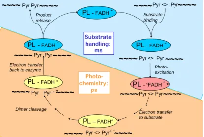
PL - FADH -PL – FADH° Pyr <> Pyr° -PL - FADH ° Pyr Pyr ° -PL - FADH -Pyr <> -Pyr PL -FADH -Pyr -Pyr PL -1FADH -* Pyr <> Pyr Pyr <> Pyr Pyr Pyr Electron transfer back to enzyme Electron transfer to substrate Dimer cleavage Photo-excitation Substrate binding Product release ~~~~ ~~~~ ~~~~ ~~~~ ~~~~ ~~~~ ~~~~ ~~~~ ~~~~ ~~~~ ~~~~ ~~~~ ~~~~ ~~~~ Photo-chemistry: ps Substrate handling: ms
Figure 3. Schematic presentation of the photorepair reaction cycle. <> symbolizes the cyclobutane ring in the CPD.
Thus, both reactions cover functionally important events in the large time window ranging from picoseconds to milliseconds, a situation that is rather typical for enzymatic catalysis
What is flash spectroscopy and what can it do ?
Simple, (relatively) cheap, versatile. In the following short review of some of our results from the last seven years, the stress will be on the versatility of flash spectroscopy and how it could be brought to help deciphering most of photolyase’s enzymatic reaction steps. The method in itself is both conceptually and technically extremely simple: a beam of (typically
monochromatic) monitoring light crosses a cell with the sample under study and its intensity
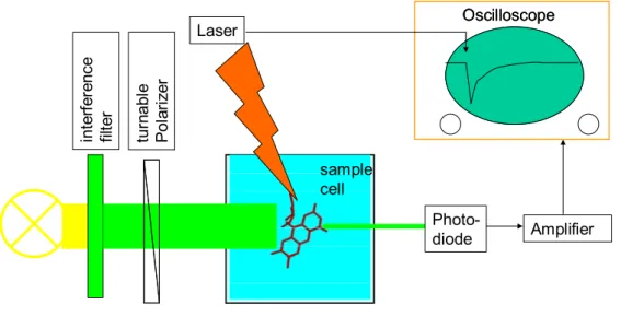
is detected continuously by a photodiode. The output of this diode is followed in time, e.g. by an oscilloscope. An intense flash triggers a reaction in the sample cell and if this reaction brings about any changes in the absorption of the participating molecules (reactants, products, solvent), they will be found as a change in the photodiode output. Such setup allows both identifying species (by their spectral signature) and following reaction kinetics (by the time course of absorption changes) (see Fig.4 and chapter 10).
sample cell in te rf er en ce fil te r Photo-diode Oscilloscope Amplifier Oscilloscope Laser tu rn abl e Pol ar iz er
Figure 4. Schematic presentation of a transient absorption (fluorescence) setup
The challenge is to develop setups that have the sensitivity to identify ever smaller changes in wavelength, amplitude or time. In reality, these things are interwoven because in the end it is photons per nm (spectral resolution) per second (temporal resolution) that are detected and if their number drowns in the unavoidable noise of the detection system, there’s nothing more to be done [9].
In the case of fluorescence spectroscopy, one can leave either of the light sources out (“Fluorescence induction”) - the actinic light will concomitantly serve to trigger the process under study and to excite the fluorescence by which you study it. Alternatively, one can use two pulses (“pump-probe”), one –actinic- to trigger and a second -delayed- for testing. This will put some demands on synchronisation, but except for some filters and lenses, the setup is very similar to that for transient absorption.
2. Photoactivation - Reducing an intraprotein flavin radical
Originally, photoreduction of FADH° by the solvent exposed tryptophan residue W306 had been found to take ~1 µs [10] and was thought to occur in a single step (or via superexchange coupling involving W382 and W359 [11]). Aubert and coworkers [12] later demonstrated by transient absorption that excited FADH° in E. coli photolyase was reduced in ~30 ps and that the previously observed much slower reaction reflected in fact deprotonation of the W306 cation radical (time constant ~300 ns). To explain the very fast electron transfer, they suggested the involvement of two intervening tryptophan residues as “stepping stones”.
How to distinguish three tryptophans in an electron transfer chain from each other ?
Taking them out one by one. That is what has been accomplished by Andre Eker at Erasmus University in Rotterdam. He replaced the three Trp residues of the putative electron transfer chain –one at a time- by isosteric but redox inert phenylalanine (Phe, F). In E.coli, the three mutant proteins can be overexpressed and isolated. The protein with the Trp proximal to the flavin replaced is called W382F, that of the intermediate Trp is W359F and that with the distal (surface exposed) Trp mutated goes under W306F.
What, if we take out the proximal tryptophan ? ([13], appendix A)
No electron transfer. The excited flavin radical won’t have the chance of electron abstraction (donor no more available) and hence will have to go back to its ground state with its intrinsic excited state lifetime. This lifetime was not known before for the FADH° radical and we measured it to be 80 ps (see Figure 5). If no donor at all is available, the direct decay will happen in 100% of the cases and no resting signal will be detectable after that time. On the picosecond timescale, this is what we observed. However, if some of the excited flavin radicals would manage to pick up an electron, e.g. from the middle Trp 359, the
recombination after subsequent electron transfer from W306 is expected to take milliseconds and can be sought for on a slower setup.
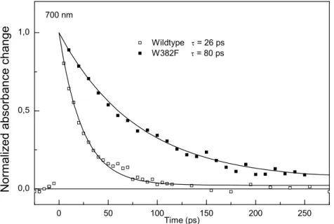
0 50 100 150 200 250 0,0 0,5 1,0 Wildtype = 26 ps W382F = 80 ps Normalized absorbance change Time (ps) 700 nm
Figure 5. Decay of the excited flavin radical in the presence (empty squares) and absence (filled squares) of an electron donor. Lines are monoexponential fits (26 and 80 ps).
Why should we see something in milliseconds if there was nothing in picoseconds ?
Because of the noise. It is in the order of 1 mOD for the ultrafast measurement. In the case of a slow measurement, we can couple the photodiode to a high-impedance, low-noise,
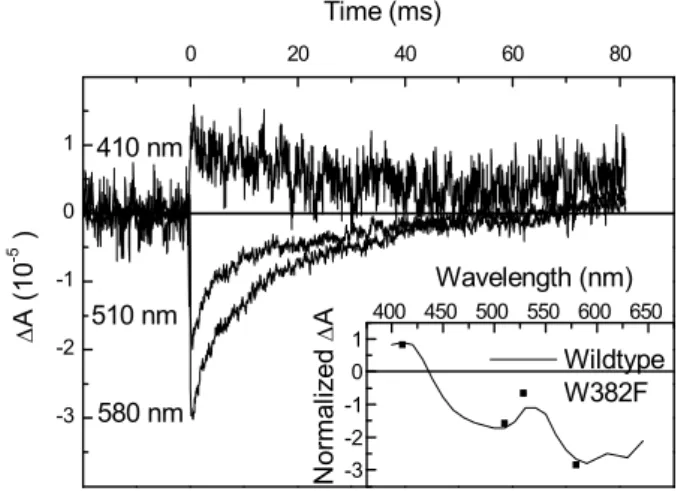
bandwidth-limited preamplifier and thus, with reasonable averaging (128 shots) make appear signals as small as 0.01 mOD. In the case of W382F mutant photolyase, this allowed to find the trace of a residual electron transfer and even determine a spectrum of the donor, leading to the conclusion that it was also a tryptophan, most likely W359 (Fig.6, inset)
Figure 6. Tiny residual absorbance changes allow to identify the electron donating species as a tryptophan (radical after donation) and estimate the yield as 0.1 ‰
What is different between W359 and W306 ? ([14], appendix B)
Their orientation. The chain FAD-W382-W359-W306 in DNA photolyase from E. coli is a prominent example of a biological electron transfer chain that contains identical molecules so that electron transfer between them does not change net absorption. The electron transfer between the tryptophan residues could previously not be monitored directly as the absorption changes due to the reduction of W382°+ and of W359°+ are compensated by those due to the concomitant oxidation of W359 and W306, respectively.
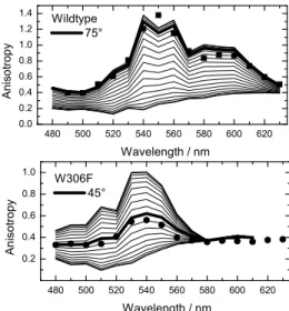
To overcome this difficulty, we made use of the fact that polarized excitation (by a pulsed laser) induces a preferential axis (that of the excited transition of FADH°) in the a priori unoriented sample (photoselection), and that the transition dipoles of oxidized W359 and W306 form different angles with this axis (known from the crystal structure, see Figure 2). Thus, polarized detection should allow distinguishing between these two chemically identical residues in their transiently oxidized state. To demonstrate this, we replaced W306 by redox inert phenylalanine, thus pruning the electron transfer chain behind W359. On a “classical” setup (time resolution 10 ns), we showed that the resulting transient absorption polarization pattern at ten nanoseconds after excitation is in line with the orientation of W359 but well different from that in wildtype photolyase where W306 is oxidized in the same time scale (Fig.7). Based on the crystal structure, the measured anisotropy for mutant and wildtype photolyases allows for an adjustment of the transition dipole moments within the molecule
frame for both flavinyl and tryptophanyl radicals [14]. Subsequently, pump-probe
measurements with picosecond resolution demonstrated that the polarization pattern at 100 ps is already that of [FADH- ,Trp306H°+], suggesting that electron transfer along the triple tryptophan chain is limited by the first step [15].
-3 -2 -1 0 1 0 20 40 60 80 -3 -2 -1 0 1 400 450 500 550 600 650 Time (ms) A ( 10 -5 ) 410 nm 510 nm 580 nm Wildtype W382F Wavelength (nm) N or m al iz ed A
Figure 7. Comparison of measured (symbols) and simulated (lines) anisotropy of initial absorbance change for photolyases with the chain ending with W306 (wt, top) or W359 (mutant, bottom) allows extracting the angle formed by the detected tryptophanyl transition with that of the excited flavin.
Two more things to keep in mind on polarization
* On a suitable timescale, the effect of photoselection can be used in transient absorption spectroscopy to obtain bigger signals, if detecting parallel to the pump pulse polarization, where the excited population is largest.
* If depolarization processes intervene on the timescale of interest, they may introduce
kinetic artefacts. These can be prevented when detecting under the magic angle (54.7°), the
squared cosine of which is 1/3, thus ensuring that always constant contributions from both polarisation directions reach the detector (meaning that a polarizer is always a good idea if you don’t know your timescales in advance).
What happens between 100 ps and 10 ns ? [16]
We can’t tell. This question is tantalizing because, with the distal Trp mutant, we see at 300 ps a protonated tryptophanyl radical and at 10 ns we see a deprotonated tryptophanyl radical. In between should happen a deprotonation, but how can we see it? For technical reasons, pump probe spectroscopy becomes unreliable for small signals at times ≥ 1 ns and “classical” transient absorption had not yet reached this limit for biological material (see chapter 3). So there was no overlap between the accessible time windows of the two techniques and this prevented us, among others, from knowing the amount of recombination occurring during the “time gap”. In this situation, we applied “kinetic overlap actinometry”. The idea is to find a substance (the “chemical actinometer”) of well-characterized behaviour on both timescales (in our case, some special red-absorbing ruthenium complex) and to measure it back-to-back with photolyase on both setups. However, complications may arise from differences between setups in experimental parameters such as excitation pulse profiles, beam geometries etc. and also from differences in absorption spectra between samples and actinometers. For this reason, even after careful correction, the accuracy of such “calibration” measurements will rarely exceed 20%. Nevertheless, we could exclude major losses during the “1 ns” time gap and hence extrapolate early yields from the more reliably defined late yields. This link in turn
480 500 520 540 560 580 600 620 0.0 0.2 0.4 0.6 0.8 1.0 1.2 1.4 An is o tr op y Wavelength / nm Wildtype 75° 480 500 520 540 560 580 600 620 0.2 0.4 0.6 0.8 1.0 Wavelength / nm A n isot ropy W306F 45°
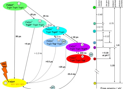
allowed to draw up a more complete scheme of the electron transfer pathways and energetics during photoactivation in E.coli photolyase, as summarized in Fig.8.
Free energy / eV < 30 ps < 9 ps 45 ps 200 ns FADH* TrpH TrpH TrpH 1 FADH WH WH WH 7 80 ps <4 ps 3 ns 25 ns 23.4 ms FADH¯ TrpH TrpH TrpH+ 5 4 FADH¯ TrpH TrpTrpH FADH¯ TrpH TrpH+TrpH 3 + H+ >0.5 µs > 1.2 ns 650 nm >25 µs 1 2 3 4 7 6 5 < 0.40 1.9 > 0.11 > 0.24 > 0.12 > 0.18 at pH 7 0.75 1.15 m idpo in t po te nt ia ls pho to ni c ex ci ta tion el ec tr on tr an sf er (d e -)p ro to na tio n FADH¯ TrpH TrpH Trp 6 FADH¯ TrpH+TrpH TrpH 2 -H+ -H+
Figure 8. Overview of electron (proton) transfer pathways during photoactivation of E. coli photolyase and their parameters as revealed by our studies [12-21].
Excitation of the flavin radical with visible light leads to its singlet excited state FADH°* whose redox potential is such that it abstracts (within 30 ps) an electron from nearby Trp382. The formed tryptophanyl radical 382TrpH°+ in turn is unstable and recombines immediately
with the reduced flavin FADH- to the neutral ground state [FADH° Trp]. A fraction (about one third) of 382TrpH°+ however succeeds in abstracting an electron from another close-by
tryptophan residue 359TrpH. Again, recombination is possible, but as the distance is now
much bigger (10 vs 4.2 Å), it competes much poorer with another forward electron abstraction step from a third tryptophan, less than four Ångstroms away, surface exposed
306TrpH. As the second and third steps are faster than the first one, the intermediate states
(382TrpH°+ and 359TrpH°+ ) are not populated in wildtype to any significant level and escape
spectroscopic detection. Direct recombination from the third Trp radical (over 15 Å) is estimated to take microseconds and is by far outcompeted by deprotonation of 306TrpH°+ to
form the neutral radical 306Trp° in 200 ns. Depending on the availability of external electron
donors, this latter can recombine in the millisecond time scale or else undergo further reduction and thus stabilize the reduced flavin.
Driving forces are calculated from spectroscopically determined rates and yields, detailed motivations can be found in [16].
3. The nanosecond hole – missing overlap between fast and ultrafast
If, however, one wants to not just exclude losses but really know what goes on around one nanosecond (e.g. the time constant for W359 deprotonation), it is necessary to create an actual overlap between the time windows accessible to fast and ultrafast measurements, respectively.
Should the “nanosecond hole” be fixed ?
Yes. Since its introduction in the fifties [22,23], flash absorption spectroscopy has become a most powerful tool in the study of light induced reactions in many fields. Based on its remarkably simple principle, it found applications in areas all over physics, chemistry and biology. The reaction is triggered by a strong actinic flash, originally created by a flashlamp and of microsecond duration. With the advent of lasers, shorter flashes (nanoseconds) became available and this extended the achievable time resolution, which was now essentially
determined by the speed of the detection/recording system. Later on, these limitations were overcome by introduction of the pump/probe technique where a slow detection system was no longer a problem because the detecting light itself was now a short pulse [24,25]. These achievements opened the pico- and femtosecond window to optical absorption spectroscopy with an overwhelming host of new and fascinating insights [26].
It is, however, often overseen that the two complementary methods, “classical” flash
absorption spectroscopy and “ultrafast” pump-probe spectroscopy do not fit with each other very neatly. Actually, rare are the cases where the latter method has proven able to detect signals of lifetimes reaching or exceeding a nanosecond, especially if those signals are small. This is due to intrinsic baseline instabilities for the very long delay lines required for
achieving nanosecond separation of pump- and probe pulses. On the other hand, “classical” setups’ time resolution has not reached the few-ns region due to both problems increasing the electronic bandwidth and additional noise arising from this increasing bandwidth. Meanwhile, this elusive 0.5-5 ns window represents a whole decade of lifetimes that are typical for electron and energy transfer processes and it is therefore highly desirable to dispose of a method that makes this “nanosecond hole” accessible.
Finally, it may be remarked that even at time scales where classical and ultrafast transient absorption techniques do overlap, they can provide complementary information as the classical technique is typically applied for multiple wavelengths, capturing all delays at one time whereas the inverse is true for pump/probe setups, thus providing for mutual baseline verification.
Can the “nanosecond hole” be fixed ? ([27], appendix C)
If the money is there. Recently, important advances and developments in detector/ amplifier/ digitizer/ laser techniques have pushed the abovementioned bandwidth limits back to a stage where it became reasonable to design a setup able to meet this challenge. It should be
mentioned here that new material at the edge of technology has its price and acquiring the parts that make up the machine presented schematically in the figure below (Fig.9) became possible thanks to the circumstance that at one precise moment in French Science, ANR had started to finance projects and CNRS had not yet ceased to do so.
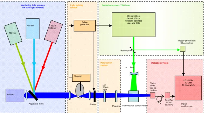
The transient absorption setup is composed of the following main elements:
a) The excitation system based on a Nd/YAG laser (Continuum Leopard SS-10) provides pulses of 100 ps duration and up to 50 mJ energy at either 532 or 355 nm at a repetition rate of 2 Hz. A small fraction of the pulse is used to trigger the detection system via a fast photodiode.
b) Four alternative continuous wave (cw) lasers provide monitoring light of rather low noise at wavelengths covering the visible spectral range: A laser diode (Nichia NDHB510) emitting up to 50 mW at 448 nm, diode pumped solid state (DPSS) lasers emitting 20 mW at 488 nm (Picarro Cyan-20) and 25 mW at 561 nm (Oxxius 561-25-COL-002), respectively, and an external cavity diode laser system (EOSI 2010) tuneable between 660 and 695 nm that emits 5-10 mW.
c) A mechanical light pulsing system limits the actinic effect of the monitoring light. A rotating plate with a small hole is placed in the focus of a collimating lens and provides monitoring light pulses of 70 µs duration at a repetition rate of 66 Hz. An additional shutter selects one out of 33 pulses to match with the 2 Hz repetition rate of the excitation laser pulses.
d) A polarization system allows turning the polarization of the monitoring light to any angle with respect to the (vertical) polarization of the excitation pulses. It is composed of an achromatic /2 waveplate optimized for 400- 700 nm (from Melles Griot) and a Glan laser linear polarizer (CLPA-10.0-425-675 from CVI).
e) The detection system is optimized for fast response, high fidelity and low noise. It consists of a Si photodiode (Alphalas UPD-200-UP; risetime, 200 ps; sensitive area, 0.1 mm2),
optionally an electronic amplifier (Femto HSA-X-2-20; 20 dB; 10 kHz – 2 GHz), and a digital oscilloscope (Agilent Infinium 81004B; bandwidth, DC – 10 GHz; sampling rate, 40
Gsamples/s). An interference filter with transmission maximum at the wavelength of the monitoring light protects the photodiode against stray light from the excitation beam and against fluorescence.
Figure 9. Scheme of a transient absorption setup with sub-ns time resolution. The detector is so small that only a focussed cw- laser can provide sufficient measuring light in the short acquisition time. Such intense measuring light is amenable to degrade the sample and must hence be chopped to minimize exposure to a short (µs) window synchronized with the excitation pulse (100 ps). 355 or 532 nm 50 mJ, 100 ps vertically polarized rep. rate 2 Hz ≥ 5 mV/div 10 GHz 40 Gsample/s Digital oscilloscope Photo- diode: 200 ps risetime Trigger-photodiode: 60 ps risetime Excitation system: YAG laser
Monitoring light sources: cw lasers (10–50 mW)
488 nm
Thermostated sample holder Polarization system Detection system /2 Wave- plate Polarizer Amplifier: 10 kHz to 2 GHz 562 nm 660 to 695 nm 448 nm Shutter Delay- generator Light pulsing system Chopper Adjustable mirror Beamsplitter cyl. lens
Is the “nanosecond hole” thus fixed ?
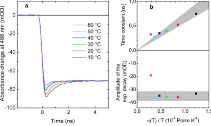
Proof. Other than constructing a setup that claims to reliably resolve kinetics around one nanosecond, we also need to have a method to verify these claims. Lifetime standards as usually used for this purpose are scarce, exactly for the reason that the time window in question has not been assessed routinely previously. We therefore resort to an adjustable lifetime standard as represented by the rotational diffusion of a small chromophore with intrinsic absorption anisotropy. For a sphere of radius R, this anisotropy decreases exponentially with a characteristic lifetime given by
= 4R3(T)/3kT, where k is Boltzmann’s constant.
Raising the temperature T of the solvent will decrease the viscosity , which, for our glycerol-water mixtures, effects much stronger than the inverse temperature dependence in the denominator and thus we are able to tune the time constant of rotational diffusion quite easily. A reassuring aspect to this method of creating standard signals is that it relies entirely on photophysical principles and is hence free of any whims of high-speed electronics.
In order to detect the limits in time and amplitude resolution of the “sub-ultrafast” setup, we first adjust the viscosity (by adding glycerol) of the dye solution such that the parallel signal decays to the isotropic value with well resolved kinetics and amplitude at room temperature. Then, by heating the sample, rotational diffusion becomes faster in a predictable manner and, as our detecting system cannot follow it any longer, the signal will increasingly lose
amplitude. Figure 10 shows that application of an exponential fit allows to recover the lost amplitude and thus the system is able to reliably resolve both lifetime and amplitude within an error margin of 10% (grey zones) down to 300 ps of expected lifetime (provided an
exponential decay is applicable).
0 2 4 -100 -80 -60 -40 -20 0 Abs o rbanc e change at 488 nm (m OD) Time (ns) 60 °C 50 °C 40 °C 30 °C 20 °C 10 °C 0,0 0,5 1,0 1,5 -40 -30 -20 -10 A m pl itude of th e ex p. d ec ay (mO D ) (T) / T (10-4 Poise K-1 ) 0,0 0,2 0,4 0,6 0,8 1,0 1,2 1,4 0,0 0,5 1,0 Tim e con st ant ( n s) b a
Figure 10. Expected decay times down to 300 ps are reasonably recovered by exponential fitting.
4. Photorepair – the ultimate challenge
What was known on photorepair ?
Structure: yes - kinetics: little. Structure Using a chemical trick (replacement of the inter-nucleotide phosphate by carbon-based formacetal ether), Carell and coworkers [28] managed to produce a CPD analogue with the right stereochemistry (in natural DNA, exclusively cis-syn is found) in sufficient amount for crystallographic studies. The complex of a double stranded DNA oligomer carrying this building block with photolyase from A.nidulans was crystallized; and one of the four protein-DNA complexes in the crystal structure actually showed the CPD tightly bound in the protein’s binding pocket, flipped out of its DNA strand, as predicted [29] (Figure 11). The only flaw was that the synchrotron radiation used for structure determination had done severe photodamage: it had repaired the cyclobutane ring and restored the intact thymines. So the result of the study was damaged CPD (=intact DNA) in the geometry of intact CPD (=damaged DNA). Presumably, the flipped-out geometry was preserved due to the low temperature (100 K) that prevented release of the DNA from the enzyme’s substrate binding pocket. This suggests that this latter process needs some thermal activation, in agreement with earlier measured positive binding energies [30].
Figure 11. The overall view of photolyase from A.nidulans in complex with a repaired substrate-analogue (1tez.pdb,[28]) shows the dimer flipped out of the double helix. One can also see that the flavin (red) is approached by antenna(orange), triple tryptophan chain (green) and substrate (blue) from different sides- a rather remarkable construction design.
For photorepair, to date, two relevant kinetic studies have been published. MacFarlane & Stanley [31] measured transient absorption at 265 nm on photolyase from A. nidulans devoid of antenna cofactor due to overexpression in E. coli. Kao et al [32] combined fluorescence upconversion (480-625 nm) with transient absorption studies at four different wavelengths (510,580, 625, 690 nm) on E. coli photolyase with the antenna cofactor depleted by photobleaching.
Whereas both studies agree on the finding of a ca 600 ps-phase and give compatible
interpretations: (splitting of the second C-C bond of the CPD in the former case and electron back transfer to the flavin radical in the latter), findings on and interpretations of the events before that (i.e. electron transfer to the CPD and splitting of the first C-C bond) differ and appear rather incompatible with each other. These discrepancies might not be too astonishing in view of the fact that different spectroscopic techniques, wavelength ranges, sample sources and preparation techniques were involved. For these same reasons, the question as to which of the studies comes to the “right” conclusions, is idle - it must rather be concluded that, based on these encouraging attempts, more thorough work is needed in order to understand the mechanistic details of photorepair.
The UV-studies [31] were actually designed to choose a particular wavelength (265 nm) where absorption increase due to CPD repair is maximal (17 mM-1 cm-1) whereas FADH-
/ FADH° difference absorption is minimized (6 mM-1 cm-1). This issue is crucial as both
contributions will occur concomitantly and with different sign upon electron transfer to the CPD. Regrettably, these studies failed to reproduce the established lifetimes of FADH-* excited state decay in the absence and presence of CPD-containing substrates (ca 1.3 vs 0.2 ns) [33] and must therefore be suspected of imperfect/incomplete substrate binding. Such binding problems should not come as a surprise here because, in order to avoid the huge background absorption of intact bases, the authors used very short strands whereas it is known that longer strands are better bound.
The studies of Kao et al. [32] concentrated on the visible wavelength range, where contributions from FADH-* (induced emission and excited state absorption) and from FADH° (formation and decay due to forward and reverse electron transfer) are expected, but CPD repair itself is not seen (marker band around 260 nm).
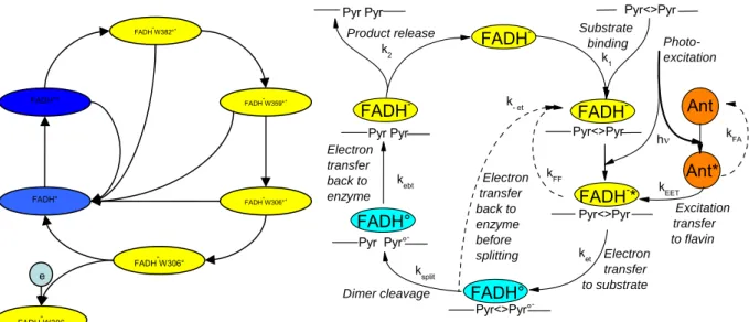
The resulting kinetic and spectral overlap of various flavin species makes it necessary to recur to a kinetic model in order to extract individual rate constants or spectral shapes. The simplest such model is represented in Figure 12, right. If antenna depletion did not leave any species behind, that could absorb at the excitation wavelength (400 nm), the antenna part of the scheme may not be considered. If, by contrast, other absorbing species are present (CPD-based intermediates, or incompetent enzyme complexes, e.g. without properly bound substrate because rebinding after repair is not yet complete or with partially oxidized cofactor because electron return was incomplete or finally with repaired substrate bound because release takes 50 µs [34], the corresponding branches need to be added to the scheme. The authors of [32] preferred a simplified analysis assuming k-et =0 (no electron back transfer before repair) and
obtained ket=170 ps for the forward electron transfer. The controls presented in that work do
not allow judging the degree to which this treatment is justified and the conclusions
warranted. On the other hand, recent steady state work on photolyases both from E. coli and A. nidulans [35] suggests that the actual quantum yield of repair might be lower than
previously assumed and hence the k-et process not negligible. Then, the alternative description
of the FADH-* decay by a sum of two exponentials with 60 and 335 ps lifetimes might be interpreted as being due to the presence of the k and k processes, but the data in [32] are not
sufficient for the assignment of individual rate constants. Again, in the simplest possible homogeneous model, a 50% quantum yield of photorepair would imply comparable rates for the productive (ksplit and ket) and the unproductive ( k-et ) channels.
Figure 12. Comparison of reaction schemes for photoactivation (left) and photorepair (right). Radical flavin is blue, reduced flavin is yellow. Photoexcitation happens into the radical during photoactivation (at 9 o’clock) and into the reduced flavin during photorepair (at 3 o’clock).
Why do we understand photoactivation better than photorepair ?
Because it is cyclic. Upon comparison of the reaction schemes for photoactivation and photorepair (Figure 12), a whole range of striking parallels hit the eye:
-both reactions cycle between FADH° and FADH-
-both excitations engage the flavin in ultrafast electron transfer -both timescales cover events from ultrafast (ps) to slow (ms)
-both schemes show branching points involving back channels at essential reaction steps -both reactions are essentially cyclic with some external in/output branches
Regardless of all these similarities, it is possible to dress a more or less complete picture of the photoactivation reaction (Figure 8) whereas for photorepair, the presented scheme rests for its better part speculative. The problem is rooted in a technical difficulty that is linked to the last of these common points: The crucial difference for studyability is, that for
photoactivation, the interactions with the environment can be eliminated by keeping the medium electron-donor-free, thus ensuring that the reaction is completely cyclic and can be repeated as often as desired. This is not possible in the case of photorepair, where substrate repair is the essential step and cannot reasonably be eliminated if it is photorepair that is to be studied. The severe limitations on the repeatability thus imposed have direct consequences for the attainable signal-to-noise ratio.
FADH° FADH°* FADH-W382°+ FADH-W359°+ FADH-W306° FADH-W306°+ FADH-W306 e Excitation transfer to flavin Ant kFA h kEET Ant* k- et Electron transfer back to enzyme before splitting kFF kebt ket ksplit Pyr<>Pyr FADH -FADH -FADH° FADH° FADH-* FADH -Pyr<>Pyr° -Pyr -Pyr° -Pyr<>Pyr Substrate binding Product release Photo-excitation Electron transfer to substrate Dimer cleavage Electron transfer back to enzyme k2 k 1 Pyr<>Pyr Pyr Pyr Pyr Pyr
What can be done about it ?
Keep trying. What we hence needed to finally see repair, is first a substrate which is well bound by photolyase on the one hand but does not obscure observation at 266 nm by its huge background absorption on the other hand. We could solve this issue by saturation of all but one of the thymines surrounding the CPD in the strand to the dihydro form. The resulting
substrate analogue is virtually UV-transparent but is bound and repaired equally well as
traditional CPD-containing oligonucleotides ([35], appendix D). In passing, we used a chemical actinometer (a dimethylamino benzenediazonium salt with a characteristic
absorption peak at 360 nm) to measure the photorepair quantum yield and found that it was about half of the “unity” established in the literature [4].
Now, extending the sub-nanosecond setup for milliOD transient absorption changes described above (see chapter 3) to application on a light-consumed sample in the UV presented in itself only few more reasons to despair. The difficulties outlined in the previous section didn’t let sleep Klaus Brettel for more than ten years. It was his unique combination of cleverness and stubbornness (call it wisdom) that let him push on, and allowed him to obtain the means to step further. So, in the fall of 2009, by adding an ultrastable 266 nm UV laser (that Sony had originally developed for their inhouse wafer technology) to the “hole fixing” setup, this
impossible setup came into existence. This was the moment I left Saclay. What does photorepair look like ?
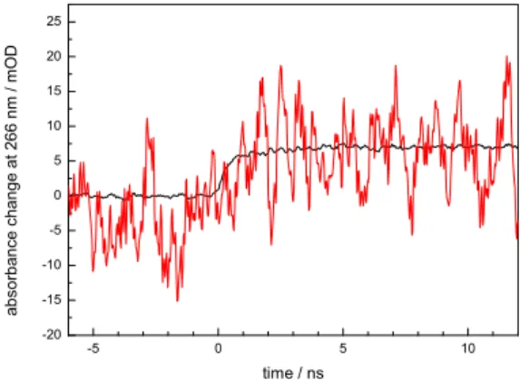
Noisy. In the last days of his Saclay postdoc contract (and of the year 2009), Thiagarajan Viruthachalam collected hundreds of individual single flashes on a photolyase sample renewed after each shot. All in all, we have 361 usable photorepair events monitored at 266 nm with 300 ps time resolution and averaging them all allowed us to make the repair signal appear out of the noise (Figure 13).
-5 0 5 10 -20 -15 -10 -5 0 5 10 15 20 25 ab sor b an ce ch ange at 2 66 nm / m O D time / ns
Figure 13. Reasonable averaging gives a usable transient (black) from single shots (red) Unfortunately, the 266 nm signal is not only -and not even to the larger part- due to
re-formation of intact thymine. Three different flavin species: FADH-, FADH-* and FADH° are also involved in photorepair and undergo transient absorption changes at this wavelength, masking the time course of the bond-splitting reactions we are interested in. Therefore, all of these “parasite” signals need to be characterized separately, at characteristic wavelengths (in the visible this time). In order to make possible comparison of signal amplitudes at various wavelengths, we again made use of the “actinometric” approach and monitored in parallel a well-defined chemical solution- Ru(bipy)3 under all conditions. This –elaborate- procedure
What can we learn from it ?
The experiment was well worth being performed. This curve features two surprises: its risetime and its amplitude. It is rewarding that we did more then just confirming a plausible scheme that was established so long ago that its justification seemed almost beyond all doubt. Beside bringing the first solid experimental evidence for the standard scheme- our
findings also introduce new grounds for discussion on further elaboration of that same scheme. -3 -2 -1 0 1 2 3 4 5 6 7 8 9 10 11 12 -0,2 -0,1 0,0 0,1 0,2 0,3 0,4 0,5 0,6 0,7 0,8 0,9 1,0 1,1 C P Ds r epai red Time (ns)
Figure 14. Enzymatic CPD repair is both slower and less efficient then anticipated by the « standard model ».
Both the slower-then-expected rise and the less-then expected amplitude can simultaneously be explained by an electron backtransfer reaction before bond splitting is accomplished. This raises a considerable challenge to computer simulations that up to now in unison found CPD splitting upon electron injection to be ultrafast (few picoseconds) [36,37]. Clearly, our repair transient does not show traces of such ultrafast chemistry. This divergence points to the longstanding difficulty of simulation protocols to adequately handle the protein environment and the whole story may serve as a reminder that even the nicest theoretical picture is not really established as long as it has not been confirmed by measurement.
SUMMARY TO THE PAST
In a review of some papers selected from my recent research activity on enzymatic
mechanisms of DNA photolyase (2003 to present, photorepair is unpublished=confidential), I demonstrated that transient absorption techniques can be pushed to reveal information on protein function on the picosecond to millisecond time scales.
« Si la matière mue me montre une volonté, la matière mue selon de certaines lois me montre une intelligence : c’est mon second article de foi. »
J.-J. Rousseau 1762, “Profession de foi du vicaire savoyard ”
PART II: PRESENT
Functional & structural protein dynamics- approaches & parameters
5. Proteins move
6. Things around the protein also move 7. Who sees what, and when?
8. The lure of single molecules
This part deals entirely with schoolbook wisdom that I acquired essentially during the last year. Therefore, it is full of references (two thirds of the total) but does not contain a single picture. The function of this part is to serve as a background for the motivation of the
following. No warranty can be given for the correctness of the information provided. In case of doubt, refer to the original literature (or just skip).
5. Proteins move
Why should I care about dynamics ?
Maybe you shouldn’t. Proteins move because of their marginal thermodynamic stability (that is the difference in free energy between unfolded and native state G is just 3 to 10 kcal/mol, [38]). And this low stability in turn is a product of all the mutations that accumulated through history - destabilizing but not killing the protein [39].
On the other hand, in condensed media, overcoming a reaction barrier becomes possible when the reactants gain the necessary energy from their coupling to the fluctuations of the surrounding bath. The last century has witnessed important advances in our understanding of the mechanism of that coupling (Arrhenius 1889 [40], Eyring 1935 [41], Kramers 1940 [42], Hynes 1980 [43]). These theories, differing in the treatment of the bath’s contribution to reaching the transition state (top of the barrier), are reasonably successful in predicting reaction rates (for a comprehensive review, see e.g. [44]). However, their application to enzymatic catalysis remains a persisting challenge, mainly due to the proteins’ complex dynamic behaviour.
Even if from a naive experimental point of view, it seems clear that enzyme flexibility is necessary for proper function (most catalysis stalls at helium temperature), we still fail to put
hand on the “mechanistic link” of how the coupling between fluctuations and reactions is
actually put to work in proteins. To illustrate this point, suffice it to cite recent statements of two eminent players in the field: On the one hand, Arieh Warshel, who -by introducing QM/MM methods- first managed to approach the problem by computer simulations, in his 2006 exhausting review [45] calls dynamical contributions to enzyme catalysis “a popular hypothesis” but, regardless of a host of simulation techniques mobilized, fails to track down these contributions. And on the other hand, at the same time, Casey Hynes in his 2008 festschrift states that “Grote-Hynes theory could be used to understand and quantify key aspects of the murky issue of dynamical effects on the catalysis” [46].
How does this show up in live ?
On an intuitive level, the crucial role of protein motion for proper functioning can be illustrated on some rather general examples:
* With enzymes serving as trans-membrane channels, it is not uncommon to observe that they function as “gates”, i.e. they open and close selectively to permit or deny access to desired or undesired molecules, i.e. filtering is done by an active motion rather than by a static “sieve” [47].
* For proteins with allosteric regulation, binding of a substrate on one place triggers a reaction on a different site within the protein. This can be understood if there were two different minima in the free energy surface, corresponding to two different conformational substates. The potential valley of the inactive conformation is preferred by the free enzyme and that of active conformation is preferred by the enzyme-substrate complex and substrate
binding liberates the energy to push the protein over the barrier from the inactive conformation to the active one. This type of functional control by protein dynamics would
be applicable to most proteins with signalling or regulatory function [48].
* Another way of dynamic control for protein function is at work for the ubiquitous class of electron/proton transferring proteins. Here, a considerable fraction of the transfer may occur through the barrier (tunnelling) and is hence exponentially dependent on distance. If protein dynamics do rapidly enough sample the conformational space, the transfer rate will be
dominated by the few situations with optimal geometries. In the contrary case of slow
sampling, many states with less favourable organization can determine the transfer rate, simply because the “good” ones may not be reached in time [49-51].
* In the case of proteins catalysing “just metabolic chemistry”, it is clear that the “pre-reaction” free enzyme should favour substrate binding and the “post-“pre-reaction” enzyme-product complex should favour enzyme-product release, with a trigger in between achieved by a conformational change sometime in the course of the reaction [52]. For the mechanism of preferential binding of substrate over product, there is discussion between proponents of “induced fit” (first binding, then conformational change) and conformational preselection (the other way round). It turns out, that these two views are two manifestations of the same
mechanism if the conformational sampling is shifted from slow to fast [53].
How do we get a grip on this mess ?
Models. Timescales. Of these examples, the latter two illustrate directly the importance of the timescales of protein dynamics for the control of the functional mechanism. The underlying dilemma common to these examples, “few good” vs. “many not-so-good”, doesn’t seem to have any general answer to it. By disrupting an optimized structure via perturbing mutations, people attempted to demonstrate the importance of a presumably optimized “prearrangement”, but found to their surprise that, although in the mutant protein substrate binding was actually hampered, the catalytic rate did not decrease significantly [54], supposedly by compensation of this “grass root” type [55].
By here, it should have become clear that part of the problem is rooted in the fact that, due to the hierarchical organization of their conformational landscape [56], proteins display
motions on an extremely wide range of timescales. The challenge is to understand how
these motions are coupled among each other and which of them are important for function. By definition, “fluctuations” are those motions that are rapid with respect to the reaction rate. As, for enzymes, the latter span a window of several orders of magnitude [57], so will do the former and it seems difficult to know a priori where and when to look for the functional part of the protein motions. Moreover, the (de-)coupling of the various timescales presents a major technical challenge for experimenters both in vitro and in silico.
For the time being, it is tempting to stick to a mechanistic picture as put forward by Vern Schramm in his excellent 2005 review [58]. According to this, the (infinitely short lived) transition state is reached when all critical atoms simultaneously reach a “near-attack conformation” or “pre-transition state”, which –due to their ps fluctuations- is quite often for any single degree of freedom but occurs only rarely in sync for all of them.
This concept was put into a somewhat more formalized form recently by Sunney Xie and coworkers at Harvard [59]. They consider a two-dimensional problem with a reaction
coordinate R and a dynamic coordinate X which is not fast with respect to the former so it
cannot be averaged out but instead is considered explicitly. The picture that arises resembles somewhat that of an antenna-reaction center complex of oxygenic photosynthesis, where the exciton has to migrate to the place of photochemistry in order to be transformed into a charge separated state. The analogy is that it is a priori not clear whether “migration” (X) or
“chemistry”(R) is rate limiting. In nature, both situations can be found and, upon closer study, it often turns out that both processes’ rates actually are not far from each other. With respect to photosynthesis, in hindsight, one could say, that this is what could be expected from
evolution, which can exercise pressure only on the slowest process in a chain. As to the
general picture of protein dynamics, the field is wider and therefore a broader spectrum of situations is imaginable.
6. Things around the protein also move
What role is played by the solvent ?
Important. But unclear. Back in 1959, Walter Kauzmann suggested that protein folding is driven by “hydrophobic interaction”, i.e. the aqueous environment is of vital importance for structural integrity [60]. On the experimental side (as with helium temperature) most protein activity stalls when isolated proteins are dried completely and it restarts when about one layer of surface water (“saturation hydration”, 20-70% of dry protein weight) is added ([61], but see also [62]). Thus water is essential for both structure and function. As to the dynamics, they appear correlated to both of them (depending on what exactly you measure), but it is not easy to establish a cause-effect relationship from these findings ([63,64], see also many others of the papers in Faraday Discuss. 2009, Vol.141).
Single fluorescent proteins flicker in a stochastic manner, their emission goes on and off. These fluctuations stop if the protein is attached to a bare glass surface (no solvent), suggesting that some flexibility is a prerequisite for the fluorescence fluctuations [65].
In 2002, again on their working horse myoglobin, Fenimore and Frauenfelder [66] introduced the concept of “solvent slaving”: essential processes in the protein have a temperature
dependence that strongly resembles that of the solvent dielectric relaxation in different solvents, seemingly independent on viscosity [67,68]. On the other hand, by the same
techniques, dynamics are found to be different for different macromolecules (protein > tRNA > DNA) in one and the same solvent [69]. These findings suggest that protein/solvent
interactions might be more subtle than just between slave and master [70].
Both simulations [71] and experimental studies of water structure and dynamics [72-74] (see chapter 7 for the scopes of various techniques) suggest that there are different “types” of water around the protein: strongly bound, loosely bound, unspecifically bound. The meaning of these types is, however, different: ordered vs disordered in structure and slow vs fast in dynamics, but recent theoretical work suggests that the kinetics of the water movement may not at all be a good indicator of the strength or order with which it is bound to the protein surface [75]. So it seems that water and its role for life will continue to be puzzling for the years to come.
Why work under cryo-conditions ?
Handle to dynamics and energetics. If the goal is observation of “living” proteins, why should we apply low temperature, certainly not a very life-near condition? [76]
For certain techniques, like electron microscopy, single molecule spectroscopy, or
synchrotron crystallography, low temperature was initially just an unavoidable evil, necessary to be able to “see anything at all”. At low temperatures, vibrations, diffusion, reactions of the samples studied are slowed down- in short; samples are made “more stable”, but this effect can also be used for the direct study of dynamics – by switching them “on” or “off”
progressively [77].
With time, techniques became more sophisticated and often low temperature, even if still being key to good resolution, is no longer absolutely necessary. But once the cryostat in place, it is tempting to use temperature as a parameter to steer experimental conditions (e.g. via the temperature dependencies of permittivity or viscosity of the solvent). Alternatively,
temperature can be used to selectively overcome a reaction barrier or to stop a reaction in front of it. Finally, measurements of yields as a function of temperature may give an access to the height of activation barriers and thus to the energetic dimension of otherwise purely kinetic measurements. The matter is complicated by the fact that in their “natural
environment”, aqueous solution, proteins should denaturate below zero [78], so there is a whole story of cryo-protection involved [79,80].
7. Methods and what they can see
The dynamic dimension
One corner and two edges. If you add the dynamical aspect to the classical dualism structure function,
you end up with a triangle, i.e. ONE new corner, but TWO new arrows: structural dynamics and functional dynamics. Of course, these are two sides to one medal, but what makes it difficult to get a grip on this medal is the fact that the methods of study for structural and functional dynamics are not generally the same. In the most popular example, the “solvent slaving” theory [66], protein function was followed by transient absorption on geminate recombination in myoglobin, while the structural part -solvent dynamics- came from dielectric relaxation. Similarly, in the other -more recent- popular case of adenylate kinase [81,82], structural fluctuations were followed by NMR and functional movements by FRET, and computer simulations had to come to help to put it all together.
Therefore, the following short review of methods is by no means exhaustive but rather meant to underline the fact that if we want to progress in understanding the “murky issue”, we will necessarily have to cover the widest accessible time range by applying as many
complementary approaches as possible [83]. In the given case, the broad multi-method approach is facilitated by the on-site presence in Grenoble of excellent expertise and facilities for most of the techniques mentioned.
Förster resonance energy transfer (FRET)
Persuasive. The historically probably oldest approach was the 1967 idea of Lubert Stryer to use the steep (sixth power) distance dependence of Förster resonance energy transfer [84] for a “spectroscopic ruler” to measure momentary distances in space between fluorescing entities [85]. The popularity of the method comes from its simple principle, but upon second sight, it may become exceedingly tricky to obtain something reliable. One major problem comes from the strong angular dependence of the underlying dipole-dipole interaction that for
unfavourable geometries can lead to complete vanishing of the signal and also introduces large uncertainty if the correct geometry (or its change in time) is not known [86]. Another problem arises if distances approach those comparable to chromophore size because then the dipole-dipole approximation is no longer valid [87,88]. Still other problems are linked to limited knowledge of the refractive index inside a protein (solution) [89]. Finally, for application to single molecule experiments, dye photophysics can pose serious limitations [90,91]. Therefore, this method is of limited value for determination of absolute distances but rather useful for detecting movements, i.e. (transient) changes in distance or angle between donor and acceptor. Thus, regardless of its numerous limitations, FRET is a method widely used for monitoring the effects of external manipulation, like, pushing or pulling a protein or DNA strand by optical or magnetic tweezers (using fluorescent beads) or scanning probe techniques.
Kinetic protein crystallography
Rare. As many proteins are functional in crystals, this is the one method that can, in principle, visualize structural dynamics directly, i.e. real movements in real time. The main problem is resolution. Very small movements occur on very fast timescales. And as these fluctuations occur in the typically 1014 molecules per crystal not in phase, their direct monitoring is out of reach for this method. Instead, the goal is to follow structural changes that are linked to function by synchronizing the molecules of the sample. There are two strategies to achieve this: “Trapping”: Stop the dynamics (by freezing) and look afterwards (eg [92]) or “Real Time” using a pump-probe scheme: trigger the reaction (e.g. by light) and determine the structure at various delays afterwards by Laue crystallography [93,94]. This puts extreme demands on crystal quality and also requires that the reaction under study can be triggered by light. Successful examples include myoglobin [95], Photoactive Yellow Protein [96], and hemoglobin [97], or -very recently- also a bacterial reaction center [98].
Dielectric relaxation
Easy. Dielectric relaxation spectroscopy is a straightforward handle to the spontaneous movements that occur in a sample. The sample is placed inside a capacitor and an external alternating electric field is applied. This field exercises a torque on the molecules of the sample that tends to orient them. Depending on their spontaneous movement, the sample molecules resist and cause a phase shift of the current across the cell with respect to the applied voltage. This reaction will be strongest at frequencies where the external field is in resonance with internal movements, allowing for the extraction of typical relaxation times. These times can then be used to extract the dipole moment or hydrodynamic radius of the probed molecule. More information on the character of a particular relaxation process can be obtained if these measurements are carried out as a function of temperature. For the case of proteins in aqueous solution, typical relaxations occur at room temperature around few picoseconds (20 GHz, “gamma”, ascribed to reorientation of bulk water) and at few
nanoseconds (10 MHz, “beta”, ascribed to protein tumbling). Between the two, several other week relaxations can be found (“delta”) and their relation to the protein-solvent interaction is a matter of debate [99,100].
Neutron scattering [101,102] and Nuclear Magnetic Resonance [103] spectroscopies
Heavy. For insight, ask Frank Gabel (04 38 78 95 73).
These two (families of) techniques measure the amount of energy that a sample exchanges with an incident beam of neutrons or with a radiofrequency magnetic field on timescales down to picoseconds. Both can be considered as “standard” techniques for observation of structure and dynamics of both protein and solvent. Their importance is partly due to the fact that they are sensitive to protons, which X-ray crystallography is practically unable to see. Moreover, both techniques have in common that directed exchange of protium for deuterium can serve to visualize selectively the (un)labelled portion of the sample or medium. The back side of the medal is that you need an isotope lab, which might not be a minor factor even if you consider the cost of the instruments alone. The enormous infrastructure required for these techniques is probably one reason why people who apply them went further into data
extraction strategies than for other techniques. As a consequence, I do not feel qualified to qualify or quantify the scope of these techniques myself in a few words and instead, I rather gave here just the references of some reviews to begin with, that appeared to me particularly readable.
Correlation spectroscopy
Not really spectroscopy. You don’t watch anything as a function of energy. What you watch is monochromatic light coming from a small spot of the sample during a long time. If the light comes from a laser and is scattered by the sample, the method is called “Photon correlation spectroscopy” (PCS) or “dynamic light scattering”, if the light is emitted by the sample itself, we have “fluorescence correlation spectroscopy” (FCS). In both cases, the time trace is compared to copies of itself from various moments in the past and the behaviour of this auto-correlation function is analyzed as function of the delay between original and copy.
Information obtainable are particle size distributions in the former case and concentrations, diffusion coefficients or photophysical behaviour in the latter [104]. Depending on the detector, time resolutions down to picoseconds are possible, for FCS however, milliseconds are more common. Using polarized excitation and detection, rotational diffusion times can be determined that exceed largely the fluorescence lifetime limiting the direct use of
fluorescence anisotropy to this end [105]. Extension to two-focus and dual-color mode recently allowed the in vivo detection of protein-substrate interaction [106].
Terahertz Spectroscopy
Phenomenological. (“T-rays”) is the spectroscopic technique that addresses the picosecond time window directly (1 THz = 1 ps-1). Due to difficulties in the development of suitable emitters and detectors, it is only relatively recently that this method came into play [107]. Probably as a consequence, with respect to applying it to protein/water dynamics, there seems to be little theoretical framework for interpretation of its results and this is rather done on a more qualitative basis [108].
Computer simulations
Impressive. Computer simulations are the ultimate method to study protein dynamics [45,109]. They allow to observe the system while you pull here and you push there and still keep everything else from unforeseen “collateral damage”, a situation the experimenter is never really confronted with. Since the introduction of combined quantum and classical treatment (“QM/MM”) by Warshel and Levitt in 1976, it even became possible to reconcile atomistic detailed description (the quantum mechanic part) with large system size (the molecular mechanic part) [110]. Still, it often seems that the best agreement of simulation with experiment is obtained if the experiment has been accomplished beforehand. Sometimes it looks as if a mean deity is not willing to let us have “everding fer noding”.
Current simulations suffer from mainly two problems: first how to create huge amounts of data (numerical restrictions) and second how to interpret them afterwards (human
restrictions). For both kinds of problem, mediation can be brought about by mutual help between man and machine and new methods are constantly being developed. In the first case, a human bias towards “interesting” events can be introduced (“accelerated dynamics”[111], “metadynamics” [112]), but the “corruption” of the “natural flow” of things raises the
problem of synchronization of the various timescales and extraction of quantities comparable to experiment.
For the second problem, getting a grip on the vast amounts of data created, various algorithms of data reduction can be employed to find the “major” changes among an ocean of tiny
fluctuations. To name but a few, there may be cited: principal component analysis [113], mezo-analysis by discretizing conformational space onto a Markov network [114], or exploitation of various “moments” (e.g. time averages) [115].
Dynamic Stokes shift
Industry. Femtosecond fluorescence upconversion is the counterpart of pump/probe
absorption [116]. As in that technique, a trigger (pump) pulse starts the reaction and a delayed monitoring pulse serves to read out the state of the system. This probe pulse is used to “gate” a crystal that, as long as the probe lasts, shifts the fluorescence of the sample to a region where it can be seen by the detector. This technique allows to follow the evolution of fluorescence emission with femtosecond resolution, i.e. faster than detector-limited “classical” real time setups or electronic-limited TCSPC. With such time resolution, it becomes possible to follow the evolution of the emitting state as it is progressively stabilized by the surrounding medium that adapts continuously to the new charge distribution of the excited state, resulting in an increasing red-shift of the emission maximum. Typically, these so-called “solvatation” processes proceed in few ps if the solvent molecules are free to rotate. In the vicinity of the protein surface, however, they can be “glued” or “stuck”, resulting in a slowing down that can be followed as long as the fluorescence lifetime lasts (typically
nanoseconds). Complemented by anisotropy measurements, information can be derived about the movements at the site of the probe. Zewail’s and other groups perfected the approach to an amazing fertility [117-125]. With respect to proteins, artificial dyes have been complemented and partly replaced by site-directed insertion of Trp via mutagenesis (if there were Trps there before, they need to be removed in order to have a single probe).
Femtosecond stimulated raman (FSR)
Wonder weapon. Really good time resolution (faster than fast, i.e. femtoseconds) is (apart from simulations) available only to optical pulses. Atomic displacements, vibrations that is, are probed in the infrared region, e.g. by stimulated Raman [126]. Put the two together and you have the impossible: high resolution in both time and frequency. The price to pay is: you need three pulses, one to trigger the reaction, one to excite the vibration and one to probe it; and two experiments: with and without the middle pulse. By taking the ratio of the probe amplitudes for the two experiments, one obtains the so-called “gain factor” as a function of time after trigger and of vibration frequency, i.e. a three-dimensional map, be it mountain contours or colours. Knowing typical intramolecular vibration band positions, it is possible to study the temporal behaviour of all of them simultaneously [127]. This is a powerful tool that seems suited best to study the fine atomic details of processes previously investigated