HAL Id: halshs-00002452
https://halshs.archives-ouvertes.fr/halshs-00002452
Submitted on 4 Aug 2004
HAL is a multi-disciplinary open access archive for the deposit and dissemination of sci-entific research documents, whether they are pub-lished or not. The documents may come from teaching and research institutions in France or abroad, or from public or private research centers.
L’archive ouverte pluridisciplinaire HAL, est destinée au dépôt et à la diffusion de documents scientifiques de niveau recherche, publiés ou non, émanant des établissements d’enseignement et de recherche français ou étrangers, des laboratoires publics ou privés.
optimal CO2-emission abatement
Minh Ha-Duong, Michael Grubb, Jean Charles Hourcade
To cite this version:
Minh Ha-Duong, Michael Grubb, Jean Charles Hourcade. Influence of socioeconomic inertia and un-certainty on optimal CO2-emission abatement. Nature, Nature Publishing Group, 1997, 390, pp.270-273. �halshs-00002452�
The influence of inertia and uncertainty upon optimal CO
2policies
M. Ha-Duong1, M. J. Grubb2, J.-C. Hourcade1
Following the UN Framework Convention on Climate Change [1], countries will negotiate in Kyoto this December an agreement to mitigate greenhouse gas emissions. Here we examine optimal CO2 policies, given long-term constraints on atmospheric concentrations. Our analysis highlights the interplay of uncertainty and socioeconomic inertia. We find that the ‘integrated assessment’ models so far applied under-represent inertia, and we show that higher adjustment costs make it optimal to spread the effort across generations and increase the costs of deferring abatement. Balancing the costs of early action against the potentially higher costs of a more rapid forced subsequent transition, we show that early attention to the carbon content of new and replacement investments reduces the exposure of both the environmental and the economic systems to the risks of costly and unpleasant surprises. If there is a significant probability of having to stay below a
doubling of atmospheric CO2-equivalent, deferring abatement may prove costly.
The problem of climate policies is stochastic in nature: we are not likely to know soon at what concentration level « dangerous interference with the climate system » [1, art. 2] would occur. An initial abatement path consistent with reaching one selected ceiling may have to be either accelerated or relaxed in the light of new scientific information. This is why the IPCC states that: « The choice of abatement paths involves balancing the economic risks of rapid abatement now (that premature capital stock retirement will later be proven unnecessary),
against the corresponding risks of delay (that more rapid reduction will then be required, necessitating premature retirement of future capital)»[2, Ch. 8]. Incorporating uncertainty into the analysis implies that the inertia of production and consumption systems becomes critical. Without inertia, the transition costs for switching from one emission path to another would be null and uncertainty would not matter so much. But in a stochastic framework, inertia has a Janus’s role: it raises both the costs of premature abatement and the costs of accelerating
1
Centre International de Recherche sur l’Environment et le Dévelopment, 1 rue du 11 novembre, F92120 Montrouge, France.
abatement if stronger action is called for after a period of delay.
Here we analyse these issues with a compact intertemporal optimisation model, DIAM, defined in Box 1. DIAM determines the least-cost CO2 emission pathway consistent with staying below a given or stochastic concentration ceiling, given assumptions concerning abatement costs; the rate r at which exogenous technical progress reduces these costs; the societal discount rate ρ (the annual rate of decline in the present value of costs and benefits incurred in the future); and the inertia in the system D. We adopt parameters lying within the range of magnitude quoted in literature for exogenous technical progress (1% per year) and for the societal discount rate (3% and 5% per year)[2, Ch. 4 & 9], and for the model of carbon accumulation. The inertia parameter D, derived from the structure of abatement costs, is the novel aspect of the model and demands more discussion. The abatement cost at time t is expressed as a quadratic function of both the degree and the rate of abatement (Box, Eq. 6). The non-linearity of costs with respect to the degree of abatement
x
is well established in the literature [2, Ch. 7 & 8]. By adding a term that depends upon the rate of abatement A (akin to the time derivative of x), the model captures inertia explicitly. Modelling studies of capital stock turnover [3] confirm that costs depend non-linearly on the rate of abatement. In Eq. 6, additive separability between permanent costs (in ca(D) x²) and adjustment costs (in ca(D) D² A²) makes it possible to explore the impact of transitional costs independently of long-run, permanent abatement costs [4]. For example, various transportation systems and urban planning patterns with very different carbon contents could have comparable operation costs; inducedinnovations cumulating over long periods could also reduce long-run costs to low levels. Nevertheless, starting one policy and then switching to another may entail high transition costs.
To test the sensitivity of our results with respect to the form of the cost function, we explore an alternative specification Eq. 6bis, where adjustment costs are solely determined by comparing A to the rate of capital depreciation in the energy sector. As long as A is lower than the 'natural' pace of replacement of capital 1/D, there are no adjustment costs and the reduction cost is proportional to x². Above that pace, costs would be multiplied by max(1, D A).
2
Energy and Environmental Programme, Royal Institute of International Affairs, 10 St James’s Sq, London SW1Y 4LE, England.
Dimensional analysis in both specifications shows that D is a duration, which can be be interpreted as the characteristic timescale of changes in the global energy system. If interpreted purely in terms of capital depreciation at rate δ, then D = (ln 2) / δ.
This approach allows us to capture crucial dynamic constraints without resorting either to the arbitrary upper bound on emission reduction rates, as in [5, 6, 7], or to the limitations associated with representing inertia purely in terms of uniformly depreciating capital stock, as in [8, 9]. DIAM gives approximately the same results as these latter models when we set D = 20 years (i.e. δ≈ 4%/yr), a reasonable average for the rate of renewal of appliances, cars, power stations, or refineries whose lifetimes range from 10 to 40 years.
But there are many other sources of inertia in the socio-economic systems that produce greenhouse gases. Time is needed to remove market and institutional barriers to the diffusion of innovations and obstacles due to imperfect information and imperfect foresight; as empirically demonstrated in [10], without specific policies, new energy sources have taken about 50 years to penetrate from 1% to only 50% of their ultimate potential. Furthermore, greenhouse gas emissions depend in part upon long-lived capital such as buildings, transport and urban infrastructures whose effects may last more than 50 years, and on the linkages between different systems, such as the complex interlinked investments in mines, ports, pipelines and power stations. Greenhouse gas emissions today are still clearly influenced, perhaps strongly, by planning and investment decisions made in the decade after the Second World War, if not before.
None of this is reflected in available ‘integrated assessment’ models. They do not represent explicitly energy-consuming infrastructure such as buildings or roads, or the linkages between different parts of supply systems. Nor do they capture issues of technology clustering or adaptive responses associated with induced
innovation, which cumulate over decades. Other critical aspects such as the dynamics of population, economic growth and induced technology development and diffusion, within and beyond the energy sector itself, may also involve very long timescales and are not captured in the current ‘integrated assessment’ models.
This difference between inertia in current modelling practice (~20 years) and the larger empirical value (~40-60 years) is thus not surprising. Consequently we
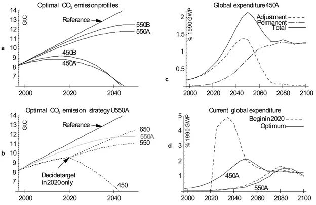
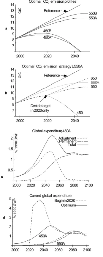
explore both 20 years and 50 years for the values of D. As Table 1 and Figure 1c illustrates, with these values, adjustment costs represent from 18% to 71% of the total cost depending upon the scenario.
We initially focus upon 450ppm and 550ppm concentration ceilings. CO2 concentrations in the range 450-500ppm - depending upon assumptions about other greenhouse gases - correspond to a total radiative forcing about double pre-industrial CO2 concentrations, which has been the benchmark for most climate model analyses of future equilibrium climate change [11]. 550ppm represents the level given greatest attention in [12]. Under the IPCC’s IS92a scenario, 450ppm is passed around 2030 and our optimal scenarios converge to this as a ceiling in 2050-60; 550ppm is passed around 2065 and converges as a ceiling in 2080-2100. Corresponding optimal pathways under different assumptions are illustrated in Figure 1(a). 650ppm is not reached until the end of the century or later.
Our main results concern the interaction of inertia and uncertainty, for trajectories in which abatement can start from 1997. The upper part of Table 1 represents optimal trajectories to a concentration ceiling known from the start, whereas the lower part represents optimal strategies when 550 ppm is the expected value of three equiprobable ultimate concentration limits of 450, 550 or 650 ppm (Figure 1b). For predetermined ceilings, the optimal trajectory is most sensitive to the ceiling. Optimal global abatement in 2020 (over and above any ‘no-regret’ measures) ranges from 19-24% for the 450ppm ceiling, and 3-7% for the 550ppm case. When 550ppm is the average of a stochastic target however, optimal
abatement is 9-14%. Furthermore the results are now quite sensitive to the assumed inertia. With D=50yrs, optimal abatement global abatement in 2020 is 11-14%; only with low inertia and high discounting does it drop below 10%. The explanation for this is to be found in the final columns of Table 1 and Figure 1 (c, d). Under a predetermined 450ppm ceiling, the major early expenditures arise from the transitional costs of turning the system away from the reference trajectory; for D=50 these amount up to 59% of the total discounted costs.
Deferring abatement requires this effort to be squeezed into a much shorter period of time, as also demonstrated in [13]. Under the 450ppm ceiling, deferring
abatement by two decades adds 70% to the total cost for D = 50, but only 32% for D = 20. As illustrated by the results for 550ppm, the costs of deferring abatement is not nearly as large when the time to stabilisation is much greater than the
characteristic time of the system. Consequently, when the ultimate target is uncertain, the costs of switching to 450 ppm pathway too late dominates costs of premature abatement in the 650 ppm case. This effect is all the more important if the resolution of uncertainties comes later (scenario U550L).
Qualitatively, our conclusions are robust to the assumed degree of inertia and discounting: even with low inertia and high discounting, corresponding to most of the models cited by [12], the abatement under uncertainty (U550B) is 9% in 2020 compared with 3% for the deterministic equivalent. But recognising higher inertia and the extent of uncertainties amplifies the economic risks associated with deferring abatement.
The results of Wigley, Richels and Edmonds [12], drawing upon various
‘integrated assessment models’ of climate change such as DICE [8] or MERGE2 [9], have been widely interpreted to support a policy of modest early abatement. Our results illustrate that abatement over the next few years is economically valuable if there is a significant risk of having to stay below ceilings that would otherwise be reached within the characteristic timescales of the systems producing greenhouse gases. Even if other greenhouse gases are strongly controlled, CO2 concentration above 500 ppm would result in atmospheric changes equivalent to at least doubling of pre-industrial CO2 levels. With continuing growth in CO2 emissions akin to the IS92a scenario, even 500ppm is likely to be passed within about 50 years. If there is any significant risk that we need to stay below this level, the socio-economic inertia in energy systems suggests that there mey be a high cost attached to a significant delay in abatement efforts. CHECK FINAL PARA.
References
1. UNFCCC. United Nations Framework Convention on Climate Change, 1992, http://www.unfccc.de/index.html.
2. IPCC Working Group III Climate Change 1995: Economic and Social Dimensions, (Cambridge University Press, 1996).
3. Hoeller, P., Dean, A. & Hayafui, M. New Issues, New Results: The OECD’s Second Survey of Macroeconomic Costs of Reducing CO2 Emissions (OECD Economic Dept. Working Paper no. 123, Paris, 1992).
4. Grubb, M. J., Chapuis T. & Ha-Duong, M. (1995). The Economics of Changing Course: Implications of Adaptability and Inertia for Optimal Climate Policy, Energy Policy, 23:4/5, 417-432 (1995).
5. Alcamo, J. & Kreilman, E. Emission Scenarios and Global Climate Protection Global Environmental Change 6:4, 305-334 (1996)
6. Enting, I. G. Analysing the Conflicting Requirements of the Framework Convention on Climate Change Climatic Change 31, 5 - 18 (1995).
7. Toth, F. L., Bruckner, T., Füssel, H.-M., Leimbach M. & Petschel-Held, G. The Tolerable Window Approach to Integrated Assessments. IPCC Asia-Pacific Workshop on Integrated Assessment Models, Tokyo, Japan, 10-12 march 1997.
8. Nordhaus, W. D. Managing the Global Commons: The Economics of Climate Change (MIT press, Cambridge, MA, 1994).
9. Manne, A. S. & Richels, R. G. Buying Greenhouse Insurance: The Economic Cost of CO2 Emissions Limits (MIT press, Cambridge, MA, 1992).
10.Andere, J., Haefele, W., Nakicenovic, N. & McDonald, A. Energy in a Finite World, (Ballinger, Cambridge MA, 1981).
11.IPCC Working Group I Stabilization of Atmospheric Greenhouse Gases: Physical, Biological and Socio-economic Implications (IPCC Technical paper III, 1997)
12.Wigley, T.M.L., Richels, R. & Edmonds, J. (1996). Economic and Environmental Choices in the Stabilisation of Atmospheric CO2 Concentrations, Nature 379, 240-243 (1996). 13.Hammit, J. K., Lempert, J. R. & Schlesinger, M. E. A Sequential-Decision Strategy for
Abating Climate Change. Nature, 357, 315-318 (1992).
14.Enting, I. G., Wigley, T. M. L. & Heimann, M. Future Emissions and Concentrations of Carbon Dioxide: Key Ocean / Atmosphere / Land Analyses (Division of Atmospheric Res., CSIRO, Australia 1994).
Box 1: DIAM, a Model on the Dynamics of Inertia and Adaptability for integrated assessment of climate change mitigation
Indices t, u refers to time periods ; s refers to states of the world. DIAM [4] finds the optimal abatement strategy x*(s, t) by minimizing total expected discounted abatement cost J defined Eq. 1. under constraints Eq. 2, the concentration ceiling and Eq. 3, dynamic
programming. Eq. 4 defines CO2 atmospheric concentration M(s, t), and Eq. 5 defines acceleration of abatement A(s, t) . Abatement costs C(s, t) are defined by Eq. 6 .
Alternatively, Eq. 6 bis is used to test sensitivity of results to the shape of the cost function. Time profile Eref(t) refers to anthropogenic fossil carbon emissions in IPCC scenario IS92a . The reference CO2 concentration path Mref(t) is computed from IS92a total carbon emission with the atmospheric perturbation CO2 response function R(u) using a linear carbon cycle [6, 14, model W]. Mref(1765), concentration before industrialization, was under 280ppmv. It was 354ppmv in 1990, increasing at 1.7 ppmv y-1. [14]
Reduction costs are determined by a social risk-free discount rate ρρρρ (3% or 5%, to account for pending controversies) ; a technical progress rate r (1%) and a characteristic time of energy systems D (20 or 50 yr). The costs scale ca(D) is normalized (ca(50)=1.36, ca(20)=3.18) so that total cost is comparable to DICE’s one [8]. Note that when Eq.6 is reported into Eq. 1, the ca(D) can get out of under the Σ , this implying that the optimal x*(s, t) is independant of ca(D).
The stochastic concentration ceiling is defined by the number of alternatives examined N ; ceilings levels L(s) ; subjective probabilities p(s) and the date of uncertainty resolution tinfo.
Results are shown Table 1. First we examine certainty scenarios N=1 for different values of D, ρ and L (sensitivity to r is mathematically the same as sensitivity to ρ). Then we explore N=3 with equidistribution over {450, 550, 650} ppmv, for tinfo = 2020 and tinfo = 2035.
(Eq. 1) J = Erreur !Erreur ! (Eq. 2) M(s, t) ≤ L(s)
(Eq. 3) ∀ t ≤ tinfo, ∀ s, 1 ≤ s ≤ N, x(s, t) = x(1, t) (Eq. 4) M(s, t) = Mref(t) - 0.471 Erreur ! (Eq. 5) A(s, t) = x(s, t) - x(s, t -1)
(Eq. 6) C(s, t) = ca(D) (1 + r) t0 - t Erreur !
[
x(s, t)² + D² A(s, t)²]
(Eq. 6 bis) C(s, t) = ca(D) (1 + r) t0 - t Erreur ![
x(s, t)² max (1, D A(s, t))
]
Table 1 : Characteristics of optimal global emissions scenarios and strategies* Certainty scenarios D yr. ρρρρ L ppmv tstab x2020 x2020 with Eq.6bis Emax GtC
tEmax Erreur ! Cost of
delay 450Aacd 50 3% 450 2060 24% 18% 8.7 2015 59% +70% 450Ba 20 5% 450 2050 19% 14% 9.2 2015 32% +32% 450C 50 5% 450 2050 20% 16% 9.1 2015 74% +72% 450D 20 3% 450 2060 23% 19% 8.8 2015 19% +25% 550Aabd 50 3% 550 2100 7% 4% 11.5 2050 55% +10% 550Ba 20 5% 550 2080 3% 2% 12.6 2050 31% +2% 550C 50 5% 550 2090 4% 2% 12.2 2050 71% +8% 550D 20 3% 550 2090 5% 4% 11.9 2050 18% +3% 650A 50 5% 650 2125 3% 0% 14.1 2070 55% +4% Hedging strategies D yr ρρρρ N tinfo x2020 x2020 with Eq.6bis x2010 E2020 GtC U550Ab 50 3% 3 2020 14% 15% 8% 9.6 U550B 20 5% 3 2020 9% 6% 4% 10.1 U550C 50 5% 3 2020 11% 12% 6% 9.9 U550D 20 3% 3 2020 12% 9% 7% 9.8 U550L (late) 50 3% 3 2035 21% 17% 12% 8.9 Footnotes to Table 1 : *
Reduction figures refer to global average (initial reductions focused on developed countries would be proportionately greater), and to reductions additional to those not incurring significant economic costs (i.e. reductions beyond no-regret measures). Column tstab shows the optimal stabilisation date, x2020 the industrial emissions abatement in 2020. (Emax , tEmax) is the optimal
emissions curve apex. Erreur ! is the share of adjustement costs in total costs, see legend for Figure 1d. The cost of delay is the increase in discounted total cost when reduction starts in 2020 instead of 1997. E2020 is the optimal emissions in 2020.
a, b, c, d
Figure 1. Optimal pathways 2000 2020 2040 7 8 9 10 11 12 13
14 Optimal CO2emission strategy U550A Reference Decidetarget in2020only 550A 450 550 650 Ct G b 2000 2020 2040 2060 2080 2100 1 2 3 4
5 Current global expenditure Optimum Beginin2020 450A % 0 9 9 1 P W G 550A d 2000 2020 2040 7 8 9 10 11 12 13 14 Optimal CO2emissionprofiles Reference 550A 550B 450A 450B Ct G a 2000 2020 2040 2060 2080 2100 0.5 1 1.5 2
Global expenditure, 450A Adjustment Permanent Total % 0 9 9 1 P W G c
Figure 1 (alternate layout). Optimal pathways under given stabilisation constraint 2000 2020 2040 2060 2080 2100 1 2 3 4
5 Current global expenditure Optimum Beginin2020 450A % 0 9 9 1 P W G 550A d 2000 2020 2040 2060 2080 2100 0.5 1 1.5 2 Global expenditure,450A Adjustment Permanent Total % 0 9 9 1 P W G c 2000 2020 2040 7 8 9 10 11 12 13
14 Optimal CO2emission strategy U550A Reference Decidetarget in2020only 550A 450 550 650 Ct G b 2000 2020 2040 7 8 9 10 11 12 13 14 Optimal CO2emissionprofiles Reference 550A 550B 450A 450B Ct G a
Legend for Figure 1
The reference case, emissions increasing linearly by about 2%/year from 1997 level,
approximates IPCC IS92a. This is assumed to be least cost without constraints, so abatement shown is global average over and above any ‘no regret’ reductions. One GtC equals
(12+2*16)/12 = 3.67 1012 kg of CO2 .
a: Four optimal emission pathways that minimise the total abatement costs for the given concentration ceiling, inertia and discount rate (see Table 1). The B cases have lower inertia and higher discount rate than A, both factors leading to higher near-term optimal emissions. However, optimal policy is more sensitive to the ultimate concentration ceiling, 450 or 550ppmv.
b: Optimal emission strategy U550A under stochastic constraint. The ultimate target is decided only in 2020, before that date, the strategy follows a precautionary path emitting sensibly less than the comparable case without uncertainty 550A.
Panels c and d, the vertical axis unit is % of 1990 gross world product (GWP), assuming the Nordhaus cost function [2]. Since D=50 for all curves in c and d, uncertainties in the cost scale parameter ca(50) would only affect curves homothetically.
c: Cost as the sum of adjustment cost and permanent cost, optimal path 450A. The ratio: area under the ‘Adjustment’ curve divided discounted by area under the ‘Total’ curve discounted is the share of adjustment costs, labeled Erreur ! in Table 1.
d: Current expenditure profiles with (dashed lines) and without (solid lines) a 20 years delay, for 450 and 550 ppm stabilisation targets (case A). For 450 ppm, cost peaks abruptly and much higher with delay than without, due to higher adjustment costs in the 2020 - 2040 period. Results are not that sharp for 550 ppm, as the time available to stabilize at 550 ppm (or above) exceeds the characteristic time of the global energy system.
CIRED
Centre International de Recherche sur l'Environnement et le Développement 1 rue du 11 Novembre, F92120 Montrouge, France.Tel: +33 1 46 12 18 72, Fax: +33 1 40 92 93 17 email:haduong@msh-paris.fr, hourcade@msh-paris.fr
your ref: G06172B PN/lcg Montrouge, le 5 August 2004 Dr. Philip Newton
Assistant Editor, Nature
Porters South, 4-6 Crinan Street, London N1 9XW Dear Philip,
We are pleased to submit the revised manuscript, retitled as ‘The influence of inertia and uncertainty on optimal CO2 policies’.
We have considered your points closely, and those of referees as asked, and we feel that we have indeed been able to address them in the enclosed manuscript:
We have shifted the emphasis of the paper to clarify the role of inertia, and why we believe that previous climate policy models have under-represented inertia. Although we show we can reproduce WRE results given the same assumptions (low inertie, 20 5% discount rate, 500ppm ceiling with no uncertainty), for the reasons set out we focus on different hypotheses, and consequently, when it comes to policy implications our views differ radically.
Accordingly, we moved the direct reference to their paper in the last paragraph, more usually devoted to the discussion of these policy implications: although discussing the adequacy of models is important, in the end the reality rules.
We think the paper meets all your editorial guidelines, as we have shortened it considerably. We have done so by dropping much of the discussion, including that of cost-benefit analysis (except for a passing reference in one sentence). We have not removed analysis of uncertainty - which we regard as central - but we have managed to shorten the discussion by integrating it with the rest of the discussion. In the same spirit, we simplified the figure representing
optimal strategies, and present it as panel b in Figure 1. Yours sincerely,
Minh Ha-Duong Michael Grubb Jean-Charles Hourcade
Enclosed :
• Revised manuscript (four copies, one with the changes clearly indicated) • Note for answering to Referee 3
Note for answering to Referee 3 about « delay is never efficient »:
The misunderstanding probably arises from the confusion between benefit and cost-efficiency models. Diam is not cost-benefit analysis. In this framework, deferring emissions can never be optimal, because it adds a supplementary constraint to the optimisation. As Referee 1 says, « it is qualitatively unsurprising, given any reasonable model of how the world works ». Here is a proof :
Proof: Let S be the set of all acceptable reduction trajectories, and let S’ be the set of all acceptable reduction trajectories that track the BAU path for one or more decade. Let J be any cost function defined over S. Then because S’ is a subset of S, the minimum of J over S is lower than the minimum of J over S’.
As we say in the paper, cost-benefit analysis is an important dimension of the issue that we have chosen not to develop here. The cost-benefit version of DIAM does actually find that deferring abatement decrease the reduction cost for lax targets and increase it for strict targets.With the functional specification in [Grubb et alii., 1995] , using a central discount rate of 4% and the same value of other parameters, we have :
D Exogenously imposed date of stabilisation
Optimal
stabilisation level
Impact of waiting until 2020 reduction cost climate damage total cost a 5 2050 488 ppmv -5% +6% +2% b 50 2050 462 ppmv +4% +16% +9% c 500 2050 459 ppmv +11% +19% +15% d 5 2150 555 ppmv -16% +6% +2% e 50 2150 516 ppmv -25% +9% +4% f 500 2150 487 ppmv -29% +12% +5%
Source : Ha Duong Minh, Comment tenir compte de l’irréversibilité dans l’évaluation du changement climatique ? Thèse de Doctorat de l’Ecole des Hautes Etudes en Sciences Sociales, Paris. En préparation.
The table shows that delay increase reduction cost only for cases b and c, when the
stabilisation date is close in time compared to the characteristic time of the energy system. This is what Ref. 3 termed a « strict » target. In all other cases a, d, e, f , the stabilisation date is far in time compared to D. These are « lax » targets, and delay is cost-efficient in the meaning that reduction costs are decreased. But note that even in this case, the idea that delay is never optimal still holds. This is because with delay, the savings in reduction costs are more than offset by the losses on climate damages.
However, to avoid the space required to explain this in full, we have dropped the reference from our paper.
Response to Referee 1:
We are glad to read that, more broadly, our paper is a part of a debate that is clearly important.
However, in our opinion, the assertion that WRE analysis does not address directly the question of inertia and optimal abatement in the near future is build upon rather restrictive definitions of ‘directly’ and ‘optimal’.
WRE raise the issue of « a realistic transition away from the current heavy dependance on fossil fuels. ». Then they present pathways that are « an idealisation of the assumption that the initial departure from the BAU would be slow ». Finally they show that « Pathways involving modest reductions below a BAU scenario in the early years followed by a sharper reduction later on were found to be less expensive ».
Those three quotations illustrate why we think about our paper as directly related to WRE. Ref. 1 points (1.) and (2.) seems to draw from the idea that we limit our paper to the remark that « deferring abatement is never optimal » and this is trivial.
First, we are unsure that the majority of Nature readership remembers that much about constrained optimisation programming. For all those, it is important to explain clearly this mathematical truth. As Ref. 3 reaction points out, the suboptimality of tracking the BAU path for a few decades is not obvious for everybody.
However, in the paper we go deeper than that. We explore quantitatively what a ‘slow’ departure from the BAU means and the cost of delay. Our approach allows to explore for what ranges of values for inertia and uncertainty WRE idealisation is more relevant than WGI.
The following loop illustrates the fundamental risk with models underestimating inertia:
Step 1. Define a reasonable target, neither too lax neither too strict. Set it according to the real intuitive socio economic inertia (for exemple, 500 ppmv if present concentration is around 360 ppmv).
Step 2. If we assume a small inertia, the target is lax.
Therefore, it is optimal to do very little reduction in the next decade: « delay is cost effective ».
Step 3. Since climate is non linear and responds with many decades lag, no damage has happened yet. Up to now, everything is fine as usual. Go back to Step 1 with 10 year more.
Jean de La Fontaine told a few centuries ago the story of the race between « The Hare and the Turtle ». If we are the turtle, we would better not adopt the hare’s strategy, especially when we don’t know how far the goal is.
Note regarding the electronic artwork provided on the disk:
The floppy disk is formatted in HD for PC, using the normal DOS file system.
Figure 1 is composed with four panels. To facilitate further publishing work, we provide two alternative layouts for them : A 2x2 block and a 1x4 column. The block was 600 points width by 371 points height, the column was 300 pts widht by 796 pts heigth.
We provide figures electronically in three formats :
• Originally, figures were generated with Mathematica 3.0 . The file figure1.nb contains the corresponding code (both layouts).
• In the paper, we used the Windows Metafile format (placeable metafile). Corresponding files are fig1square.wmf and fig1column.wmf.
• We exported to Adobe Illustrator format. Corresponding files are fig1square.ai and fig1column.ai.
Minh Ha-Duong is responsible for these figures. Please do not hesitate to contact him directly if you need supplementary information or material. Mail at haduong@msh-paris.fr, or phone at +33 146 12 18 71.