HAL Id: hal-02172934
https://hal.archives-ouvertes.fr/hal-02172934
Submitted on 4 Jul 2019
HAL is a multi-disciplinary open access
archive for the deposit and dissemination of
sci-entific research documents, whether they are
pub-lished or not. The documents may come from
teaching and research institutions in France or
abroad, or from public or private research centers.
L’archive ouverte pluridisciplinaire HAL, est
destinée au dépôt et à la diffusion de documents
scientifiques de niveau recherche, publiés ou non,
émanant des établissements d’enseignement et de
recherche français ou étrangers, des laboratoires
publics ou privés.
Degree-based Outlier Detection within IP Traffic
Modelled as a Link Stream
Audrey Wilmet, Tiphaine Viard, Matthieu Latapy, Robin Lamarche-Perrin
To cite this version:
Audrey Wilmet, Tiphaine Viard, Matthieu Latapy, Robin Lamarche-Perrin. Degree-based Outlier
Detection within IP Traffic Modelled as a Link Stream. Computer Networks, Elsevier, 2019, 161,
pp.197-209. �10.1016/j.comnet.2019.07.002�. �hal-02172934�
Degree-based Outlier Detection within IP Traffic
Modelled as a Link Stream
Audrey Wilmet
∗, Tiphaine Viard
‡, Matthieu Latapy
∗, Robin Lamarche-Perrin
†∗Sorbonne Universit´e, CNRS, Laboratoire d’Informatique de Paris 6, LIP6, F-75005 Paris, France †Institut des Syst`emes Complexes de Paris ˆIle-de-France, ISC-PIF, UPS 3611, Paris, France
Email: [email protected]
‡Discrete Optimization Unit, Riken AIP, Tokyo, Japan, [email protected]
Abstract—This paper aims at precisely detecting and identi-fying anomalous events in IP traffic. To this end, we adopt the link stream formalism which properly captures temporal and structural features of the data. Within this framework, we focus on finding anomalous behaviours with respect to the degree of IP addresses over time. Due to diversity in IP profiles, this feature is typically distributed heterogeneously, preventing us to directly find anomalies. To deal with this challenge, we design a method to detect outliers as well as precisely identify their cause in a sequence of similar heterogeneous distributions. We apply it to several MAWI captures of IP traffic and we show that it succeeds in detecting relevant patterns in terms of anomalous network activity.
I. INTRODUCTION
Temporal and structural features of IP traffic are and have been for several years the subject of multiple studies in various fields. A significant part of this research is devoted to detecting statistically anomalous traffic subsets referred to as anomalies, events or outliers. Their detection is particularly important since, in addition to a better understanding of IP traffic characteristics, it could prevent attacks against on-line services, networks and information systems.
Due to the temporal and structural nature of IP traffic, de-veloped methods can be classified into two categories: those based on signal processing [7], [10], and those based on graph theory [27], [50]. However, methods within these areas lead to a loss of information: by considering interactions as a signal, the structure is aggregated; with graphs, the temporal order of interactions is lost. Hence, existing methods struggle to identify subtle outliers, which are abnormal both in time and structure. Moreover, when they succeed, the loss of information leads to a decrease of accuracy. In this paper, we model IP traffic as a link stream which fully captures both the temporal and the structural nature of traffic [28], [44]. Then, we introduce a method in order to detect subtle outliers and precisely identify which IP addresses and instants caused it. More specifically, a link stream L is defined as a set of instants T , a set of nodes V (IP addresses) and a set of interactions E (communication between IP addresses over time). Within this framework, we focus on one key property: the degree of nodes. This feature is highly heterogeneous, which raises challenges for its use in outlier detection, but it is stable over time. Our method takes advantage of this temporal homogeneity: it divides the link stream into time
slices and then performs outlier detection to find time slices which exhibit unusual number of nodes having a degree within specific degree classes. Then, in order to isolate responsible IP addresses and instants on which they behave unexpectedly, we design an identification method based on an iterative removal of previously detected events. Finally, we validate our method by showing that these event removals do not significantly alter the underlying normal traffic.
This paper is an extended version of the work published in [49]. In this contribution, special attention is paid to the importance of parameters involved in the method such as time slice and degree class sizes. Moreover, in addition to our previous work in which we evaluated our method on a one-hour long IP traffic trace of June 2013, we apply it on two other datasets: a one-day long IP traffic trace of June 2013 and a fifteen-minutes long IP traffic trace of November 2018 which possesses a list of abnormal events indexed by MAWILab to which we compare our results [17].
The paper is organised as follows. We overview the related work in Section II and present our contributions in Section III. We introduce IP traffic modelling as a link stream and the degree definition in Section IV. In Section V, we describe our goals and the challenges they raise. This leads to the development of our method to detect events in Section VI and to identify them in Section VII. We discuss our results in Section VIII. Subsequently, we apply our method on other datasets in Section IX. Then, we investigate the influence of different time slice sizes and different class constructions in Section X. We conclude in Section XI.
II. RELATEDWORK
Techniques for anomaly detection in IP traffic are extremely diverse. Among those, methods using principal component analysis [26], [40], machine learning [48], data mining [29], signal analysis [7], [10] and graph-based techniques have been proposed. In this paper, we focus our related work on methods based on dynamic graphs. In this domain, authors traditionally study a sequence of graphs {Gi}i=1..k, such
that each snapshot Gi = Giτ..(i+1)τ contains interactions
aggregated over time window Ti = [iτ, (i + 1)τ [. Then,
they attribute an abnormality score to each snapshot Gi by
comparing it to others. This problem has been approached in various ways depending on the definition of the abnormality
score (for surveys, see [4], [39]).
Compression-based abnormality scores analyse the
evolution of the encoding cost of each graph to detect anomalies. Sun et al. [43] and Duan et al. [15] group similar consecutive snapshots into a chain. If the adding of a graph greatly increases the description length of the chain, the corresponding snapshot is considered as abnormal. Chakrabarti et al. [12] use a similar technique but apply it on clusters of nodes to find abnormal links.
Other approaches use tensor decomposition. Ide et al. [23] and Ishibashi et al. [24] build a past activity vector from the main eigenvectors associated to all snapshots within a given
time window. Then, snapshot Gi is identified as abnormal
when the distance between the past activity vector and Gi’s
main eigenvector exceeds a certain threshold. Akoglu et al. [3] use a similar technique in which the past activity vector includes nodes local features.
Outliers can also be found by studying communities evolution. Aggarwal et al. [2] find anomalous snapshots by comparing their clustering quality. Gupta et al. [20], [19] calculate the variation in the probability of belonging to a community for each node between two consecutive snapshots. Nodes for which the variation deviates significantly from the average variation of nodes within the same community are considered abnormal. Chen et al. [14] and Araujo et al. [5], in turn, detect abnormal communities among clusters which unusually increase, merge, decrease or split.
Finally, a significant amount of work quantify the distance between snapshots using graph features. Pincombe et al. [36] and Papadimitriou et al. [35] define a series of topological aggregated features to compare snapshots. Berlingerio et al. [9] use the moments of an egonet feature – e.g., degree, clustering coefficient – calculated on each node. Saxena et al. [41] use a similar method but decompose each snapshot into k cores to consider global features as well. Schieber et al. [42] use the Jensen-Shannon divergence and a measure of the heterogeneity of each graphs in terms of connectivity distance between nodes. Finally, Mongiovi et al. [33] find clusters of anomalous links by calculating, for each link, its probability to have a given weight according to its usual behaviour.
However, these techniques lead to a loss of information: by reducing interactions into a sequence of graphs, the links order of arrival within a time window is lost. To overcome this issue, other work propose to improve these methods by introducing sequences of augmented graphs. For instance, Casteigts et al. [11] and Batagelj et al. [8] use graphs in which links are labelled with their instants of occurrence. Likewise, in [6], [46] and [47], authors use causal graphs in which two nodes are linked together if there is a causal relationship between them. In this paper, we adopt a new perspective. We consider temporal interactions as a separate object called a link stream, using the formalism developed by Latapy et al. [28]. While methods for covering relevant and subtle events often go hand in hand with very complicated
features, we show that we can find relevant structural and temporal outliers, as well as gain accuracy, with a very simple feature defined in the link stream formalism: the instantaneous degree of nodes over time.
Other authors detect outliers using this modelling. Yu et al. [51] calculate the main eigenvector of the ego-network of each node and find abnormal nodes among those experiencing a sudden change in the amplitude and/or direction of their vectors. Manzoor et al. [31] use a similar technique. They store the link stream in a sketch built from the ego-networks patterns of each node and label a new edge as abnormal if the difference between the sketch before its arrival and the one after is significant. Ranshous et al. [38] also use sketches. They store the link stream in a Count Min sketch that approximates the frequency of links and nodes. From this sketch, they assign an abnormality score to each link (u, v, t) based on prior occurrences, preferential attachment and mutual neighbours of nodes u and v. Eswaran et al. [16] also rely on approximations and attribute a score to every new edge arriving in the stream by relying on a sub-stream L0 sampled from past edges. If the new edge connects parts of L0 which are sparsely connected, then it is considered as abnormal. Finally, Viard et al. [44] find anomalous bipartite cliques using the link stream formalism developed in [28].
A large proportion of the methods cited above is devoted to find globally anomalous instants (as abnormal snapshots). Among those extracting local features on nodes or links, either authors use similarity functions which aggregate local information, or they rely on approximations as samples or sketches. In the first case, instants are abnormal based on their local patterns but information about which sub-graphs are responsible is lost. In the second case, approximations allow a fast processing but lead to a decrease of accuracy. In contrast, our method identify abnormal couples (t, v) exactly, without any information loss and still exhibits fast and efficient processing.
III. CONTRIBUTIONS
We model IP traffic with a link stream and study one of its most important properties, the degree of nodes over time. We show that, although this property follows a very heterogeneous distribution that is hard to model, this distribution is stable over time. We then design a method that exploits the stability of this heterogeneity for anomaly detection, and may be applied in various such situations. This method first splits traffic into time slices and computes the degree distribution in each slice. By comparing these distributions, the method then points out degree classes and time slices such that having a degree in this class during this slice is anomalous. Using this information, we identify IP addresses and time periods involved in anomalies, as well as the corresponding traffic. By removing this traffic from the original data, we validate our identification by noticing that we turn back to a normal
(a) a b c 0 2 4 6 time (b) dt (b ) 1 2 0 0 2 4 6 time
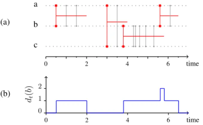
Fig. 1: Link stream for the modelling of IP traffic - (a)
Example of a link stream L = (T, V, E) formed from the
set of triplets D = {(1, a, b), (1.5, a, b), (3.5, a, c), (4.3, b, c), (4.4, b, c), (4.6, b, c), (4.9, b, c), (5.3, b, c), (6.1, a, b)}: T = [0, 7[, V = {a, b, c}, E = ( [0.5, 2[ ∪ [5.5, 6.5[ ) × {ab} ∪ [3, 4[ × {ac} ∪
[3.8, 5.8[ × {bc}. In the example, a interacts with b from t1 = 0.5
to t2= 2. (b) Time evolution of the degree of node b.
traffic with respect to the degree. We illustrate the method and its outcome on MAWI public IP traffic.
IV. TRAFFICMODELLED AS ALINKSTREAM
IP traffic consists of packet exchanges between IP addresses. We use here one hour of IP traffic capture from the MAWI archive1 on June 25th, 2013, from 00:00 to 01:00. We
denote this trace by a set D of triplets such that (t, u, v) ∈ D indicates that IP addresses u and v exchanged a packet at time t. The set D contains 83, 386, 538 triplets involving 1, 157, 540 different IP addresses.
We model this traffic as a link stream L in order to capture its structure and dynamics [28]. Nodes are IP addresses involved in D and two nodes are linked together from time t1 to time
t2 if they exchanged at least one packet every second within
this time interval. Formally, L = (T, V, E) is defined by a time interval T ⊂ R, a set of nodes V and a set of links E ⊆ T × V ⊗ V where V ⊗ V denotes the set of unordered pairs of distinct elements of V , denoted by uv for any u and v in V (thus, uv ∈ V ⊗ V implies that u, v ∈ V and u 6= v, and we make no distinction between uv and vu). If (t, uv) ∈ E, then u and v are linked together at time t. In our case, we take E = ∪(t,u,v)∈D [t − ∆2, t +
∆
2] × {uv}
with ∆ = 1s. Other choices can be made. For instance, we can set a value of ∆ that is different for each uv, or each link (t, uv), using external knowledge. We can also use a value of ∆ that changes over time (see for instance the work of L´eo et al. [30]). These operations are depicted in Figure 1.a. The degree of (t, v) ∈ T × V , denoted by dt(v), is the number
of distinct nodes with which v interacts at time t: dt(v) = |{u : (t, uv) ∈ E}|. 1http://mawi.wide.ad.jp/mawi/ditl/ditl2013/ [25]
Figure 1.b shows the degree of node b over time. Notice that the degree of b is not its number of exchanged packets over time; it accounts for its number of distinct neighbours over time.
V. HETEROGENEITY OFDEGREES
In order to find outliers in a link stream using the degree, we first need to characterize the normal behaviour of the set
of observations O = {dt(v) : (t, v) ∈ T × V }. Then, an
outlier is a couple (t, v) ∈ T × V which has a significantly different degree from others.
For this purpose, we call degree distribution of L the fraction f (k) of couples (t, v) ∈ T × V for which dt(v) = k, for all
k ∈ N:
f (k) = |{(t, v) ∈ T × V : dt(v) = k}|
|T × V | .
Figure 2 shows that the degree distribution is very
heterogeneous, which discards the hypothesis of a normal behaviour. In this situation, one may hardly identify values of degree that could be considered anomalous.
A solution is to fit this distribution, and then find values which deviates from the model. Given its heterogeneity, one may think that it is well fitted by a power law distribution P (k) ∝ k−α where α > 1 and kmax > k > kmin > 0.
However, we show that this is not the case following the procedure proposed by Virkar et al. [45]. Results show that differences between the empirical distribution and the estimated model cannot be attributed to statistical fluctuations, which leads us to reject the hypothesis that the degree is distributed according to a power law distribution.
10−16 10−14 10−12 10−10 10−8 10−6 10−4 10−2 100 101 102 103 104 105 Fraction of (t, v ) s.t. dt (v ) = k Fraction of (t, v ) s.t. dt (v ) > k Degree k
Fig. 2: Degree distribution and complementary cumulative de-gree distribution in L. For all (t, v) ∈ T × V , we compute
the degree dt(v) and plot the distribution of the set of values
O = {dt(v) : (t, v) ∈ T ×V }. The fraction expresses the probability
to draw a time instant t ∈ T and a node v ∈ V such that dt(v) = k.
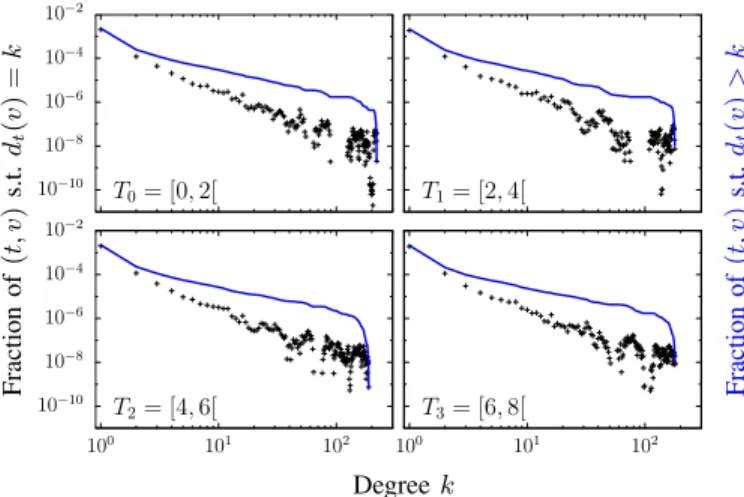
This shows that finding outliers in this type of distribution is not trivial. In order to circumvent this issue, we observe degrees on sub-streams corresponding to IP traffic during time
10−10 10−8 10−6 10−4 10−2 T0= [0, 2[ T1= [2, 4[ 10−10 10−8 10−6 10−4 10−2 100 101 102 T2= [4, 6[ 100 101 102 T3= [6, 8[ Fraction of (t, v ) s.t. dt (v ) = k Fraction of (t, v ) s.t. dt (v ) > k Degree k
Fig. 3: Degree distribution and complementary cumulative
degree distribution over 2-second time slices. For T0= [0, 2[,
T1 = [2, 4[, T2 = [4, 6[ and T3 = [6, 8[, we compute the degree
dt(v) for all (t, v) in the corresponding sub-stream and plot the
distribution of the set of values Oi = {dt(v) : (t, v) ∈ Ti× V }, for i = {0, 1, 2, 3}. The fraction expresses the probability to draw a
time instant t ∈ Tiand a node v ∈ V such that dt(v) = k.
slices of duration τ = 2.0s. Formally, we call Ti= [2i, 2i + 2[
the ith time slice, for all i ∈ {0, . . . , 1799}, and we define
fi(k) =
|{(t, v) ∈ Ti× V : dt(v) = k}|
|Ti× V |
,
the degree distribution of the ith time slice. Figure 3 shows that these distributions still are heterogeneous.
Nonetheless, Figure 3 also shows that degree distributions fi
have similar shapes. To quantify this similarity, we perform two-sample Kolmogorov-Smirnov (KS) tests on all pairs of distributions (fi, fj)i6=j [37]. According to the relative
position between the KS distance Di,j and a critical value
c, this test assess whether two samples may come from the same distribution or not. Let m = kimax and n = kjmax, be
the sizes of the two samples. With a significance level of
0.1, c = 1.073qn+m
nm [1]. Figure 4 shows the ratio between
Di,j and c. Most Di,j are below c. This means that most
samples Oi= {dt(v) : (t, v) ∈ Ti× V } are drawn from the
same distribution. On the contrary, some of them are different from all others which in turn, indicate changes in the overall behaviour on particular sub-streams.
Using these observations, we design below an outlier detec-tion method based on the temporal homogeneity of heteroge-neous degree distributions.
VI. LEVERAGINGTEMPORALHOMOGENEITY TODETECT
EVENTS
The above observations lead to the following conclusion: degree distributions are heterogeneous in the same way on most, if not all, time slices. In other words, in each time slice, the fraction of couples (t, v) that have a given degree is
0 0.02 0.04 0.06 0.08 0.1 0.12 0.14 0.16 0.18 −0.5 0 0.5 1 1.5 2 2.5 3 3.5 4 4.5 5 Fraction of (f i ,f j )i6= j Ratio Di,j/c
Fig. 4: Similarity of degree distributions over 2-seconds time slices. For all pairs of degree distributions (fi, fj)i6=j, we compute
the ratio between the KS distance Di,j and the critical value c.
We plot the distribution of the set of ratios Di,j/c for i, j ∈
{0, . . . , 1799}, i 6= j. We can see that most values are below 1 meaning that most KS distances are smaller than c. Accordingly, based on the two sample KS test, most degree distributions are similarly distributed. On the other hand, 1% of the ratios are larger than 1, which is the result of the comparison between some deviating distributions and all others.
similar to this fraction in other time slices. This is what we will consider as normal. Anomalies, instead, correspond to significant deviation from the usual fraction of nodes having a given degree. In this section we describe our method to compare degree distributions on all time slices and its use for outlier detection.
First, notice that it makes little sense to consider the fraction of couples (t, v) having a degree exactly k when k is large: having degree k − 1 or k + 1 makes no significant difference. Therefore, to increase the likelihood of observing values in the tail of the distribution, we define logarithmic degree classes Cj and consider the fraction of couples (t, v) having degrees
in Cj, for all j:
fi(Cj) =
|{(t, v) ∈ Ti× V : dt(v) ∈ Cj}|
|Ti× V |
.
We define the jthdegree class, Cj = {dkje, . . . , bkj+1c − 1}
such that k1 = 1 and log(kj+1) = log(kj) + r
where r = 0.1 is the degree class size. This leads to
C1 = {1}, C2 = {2}, C3 = {3}, C4 = {4, 5}, etc.,
until C41 = {19953, . . . , 25117}. Then, to compare degree
distributions, we plot for a given degree class C, the distribution on all time slices Ti of the fraction fi(C). In
other words, we study how the fraction of couples (t, v) which have a degree within C during Tiis distributed among
all time slices.
Figure 5 shows the distributions for classes C1, C2, C19,
C22, C31 and C41. In accordance with temporal homogeneity,
we can see that most fractions are distributed around the mean and that only a few are distant from it. As expected
0 0.1 0.2 0.3 0.4 0.5 5.0 · 10−31.0 · 10−21.5 · 10−22.0 · 10−22.5 · 10−2 Fraction of Ti s.t fi (C 1 ) = x Fraction x of (t, v) ∈ C1 C1= {1} 0 0.02 0.04 0.06 0.08 0.1 0.12 0.14 8.0 · 10−5 1.2 · 10−4 1.6 · 10−4 Fraction of Ti s.t fi (C 2 ) = x Fraction x of (t, v) ∈ C2 C2= {2} 0 0.02 0.04 0.06 0.08 0.1 0.12 0 5.0 · 10−7 1.0 · 10−6 1.5 · 10−6 2.0 · 10−6 Fraction of Ti s.t fi (C 19 ) = x Fraction x of (t, v) ∈ C19 C19= {126, . . . , 158} 0 0.1 0.2 0.3 0.4 0.5 0.6 0.7 0.8 0.9 1 0 2.0 · 10−74.0 · 10−76.0 · 10−78.0 · 10−7 Fraction of Ti s.t fi (C 22 ) = x Fraction x of (t, v) ∈ C22 C22= {252, . . . , 315} 0 0.1 0.2 0.3 0.4 0.5 0.6 0.7 0.8 0.9 1 0 2.0 · 10−7 4.0 · 10−7 6.0 · 10−7 Fraction of Ti s.t fi (C 31 ) = x Fraction x of (t, v) ∈ C31 C31= {1996, . . . , 2510} 0 0.1 0.2 0.3 0.4 0.5 0.6 0.7 0.8 0.9 1 0 2.0 · 10−7 4.0 · 10−7 6.0 · 10−7 8.0 · 10−7 Fraction of Ti s.t fi (C 41 ) = x Fraction x of (t, v) ∈ C41 C41= {19953, . . . , 25118}
Fig. 5: Distributions of fractions fi(C) on all time slices Tifor degree class C in {C1, C2, C19, C22, C31, C41} - Distributions on C1,
C2 and C19 are homogeneous with outliers. These classes are labelled as AN -classes. Distributions on C22, C31 and C41 are peaked on
zero since in most time slices there are no couple (t, v) in the corresponding class. They are labelled as A-classes.
according to the heterogeneity of degrees, the higher the degree class, the lower the fraction of couples (t, v) within the class. We see on C1 that the average fraction over all
time intervals is 2.1 · 10−3. When switching to C2, it drops
to 1.15 · 10−4 and gradually decreases to reach 0 in classes of degrees above 252. In these high degree classes, the spike on fraction 0 indicates that in most time slices, there is no couple (t, v) reaching such high degrees. Note that this is a peculiarity of this dataset, one or multiple nodes could have a constant high degree and lead to a nonzero average fraction (see Section IX). In the following, we will refer to these classes as A-classes since they only contain abnormal traffic. In opposition, classes having an average fraction greater than 0, which contain abnormal traffic and normal traffic, will be referred to as AN -classes.2
In order to validate fractions fi homogeneity over time
slices within each degree class, we fit their distributions
with a normal distribution model P (x) = √1
2πσ2e −1 2( x−µ σ ) 2
where values are normally distributed around a mean µ with a standard deviation σ. Deciding whether a given distribution is homogeneous with outliers or not may be done as follows [27]: (1) Iteratively remove outliers from the distribution with Grubbs test [18]; (2) Fitting the resulting distribution with the normal model; (3) Evaluate the goodness of the fit. We use Maximum Likelihood Estimation (MLE) to determine which model parameters fit the best the empirical
2In practice, we do not observe homogeneous classes without outliers, hence
the lack of N -classes.
0 0.02 0.04 0.06 0.08 0.1 0.12 0.14 8.0 · 10−5 1.2 · 10−4 1.6 · 10−4 Fraction of Ti s.t fi (C 2 ) = x Fraction x of (t, v) ∈ C2 After Grubbs’test Before Grubbs’test Fit KS 0.04566
Fig. 6:Fit of fractions distribution on C2 after removing outliers with Grubbs test - The KS distance between the fit and the empirical distribution is below the critical value. Hence, this distribution is flagged as an homogeneous distribution with outliers (AN -class).
distribution and evaluate the goodness of the fit with the KS test between empirical and estimated distributions. In this framework, we find 37 distributions that are homogeneous with outliers among the 41 corresponding to each degree class (see Figure 6). The remaining 4 classes are discarded from the study, we call them R-classes for rejected classes. One may use more complex and accurate techniques to automatically perform the fit, see for instance the work performed by Motulsky et al. [34].
Given an homogeneous distribution with outliers, we use here the classical assumption that a value is anomalous if its distance to the mean exceeds three times the standard
deviation [13], [21]. In classes displayed in Figure 5, we obtain 151 time slices flagged as anomalous in the first class
containing degree 1 only, 5 anomalous time slices in C2
and 12 in C19. In A-classes, peaked on 0, anomalous values
correspond to all values greater than 0.
All in all, our method for event detection from degree distributions is the following: we group degree values into degree classes of logarithmic width. For a given degree class C, we look at the distribution on all time slices of the fraction fi(C). This distribution indicates anomalous values which
means that there are anomalous high numbers of couples (t, v) having degree within C during specific time slices Ti.
We then call an anomalous value of this kind a detected event and denote it (C, Ti).
A detected event gives two pieces of information: the time
slice Ti on which the anomalous value has been observed,
and the degree class C in which the couples responsible for the high fraction are located. At this stage, we detected 1,358 such events. However, a time slice and a degree class are not sufficient information to accurately characterize the anomaly. We now address the goal of identifying couples (t, v) in T ×V responsible for these detected events.
VII. ITERATIVEREMOVAL TOIDENTIFYEVENTS
A detected event (C, Ti) is a degree class C and a time
slice Ti such that the fraction fi(C) is unusually high
compared to the ones in other time slices. Identifying this event means recovering the set I(C, Ti) of couples (t, v)
responsible for this anomaly. In this section, we introduce an iterative removal method and show that it leads to such identification.
Let us take event (C2, T1080) as an example. We have access
to the set of couples (t, v) which have a degree in C2 during
T1080. However, we cannot directly identify the event by this
set. Indeed, let us consider the new link stream L0 in which we removed the corresponding interactions: L0 = (T, V, E0) with E0 = E \ {(t, uv) : t ∈ T1080 and dt(v) ∈ C2}. We see
in Figure 7 that the removal of this set of interactions from the link stream causes the appearance of a negative outlier3 in the distribution of fractions on C2. Thus, by removing all
interactions (t, uv) such that couples (t, v) have degree in C2
during T1080, we removed anomalous traffic but also normal
traffic. Therefore, identifying the detected event (C2, T1080)
as the set I(C2, T1080) = {(t, v) : t ∈ T1080 and dt(v) ∈ C2}
is not accurate enough.
This suggests that one cannot directly identify couples acting abnormally in AN -classes. Indeed, in these classes, the normal fraction is greater than zero. Hence, an anomalous fraction consists in anomalous couples but also normal ones, which prevents us from identifying responsible couples
3We call negative outlier an outlier which is lower than the mean.
0 0.02 0.04 0.06 0.08 0.1 0.12 0.14 8.0 · 10−5 1.2 · 10−4 1.6 · 10−4 Fraction of Ti s.t fi (C 2 ) = x Fraction x of (t, v) ∈ C2 Before removal T1080 0 0.02 0.04 0.06 0.08 0.1 0.12 0.14 0 4.0 · 10−5 8.0 · 10−5 1.2 · 10−4 1.6 · 10−4 Fraction of Ti s.t fi (C 2 ) = x Fraction x of (t, v) ∈ C2 After removal T1080
Fig. 7: Incorrect identification in AN -classes - The removal of all interactions (t, uv) such that dt(v) is in C2 during the detected
time slice T1080 causes the appearance of a negative outlier. Note
that the resulting fraction on T1080 is not zero since the removal of some interactions has decreased the degree of nodes in higher classes
which end up having a degree in C2.
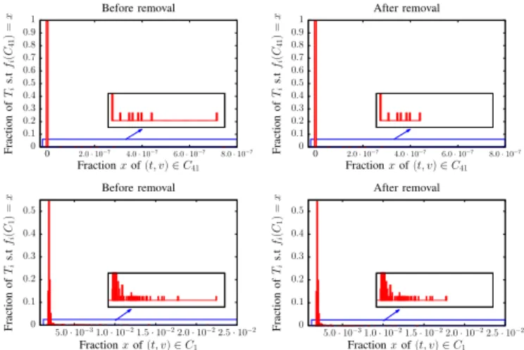
0 0.1 0.2 0.3 0.4 0.5 0.6 0.7 0.8 0.9 1 0 2.0 · 10−7 4.0 · 10−7 6.0 · 10−7 8.0 · 10−7 Fraction of Ti s.t fi (C 41 ) = x Fraction x of (t, v) ∈ C41 Before removal 0 0.1 0.2 0.3 0.4 0.5 0.6 0.7 0.8 0.9 1 0 2.0 · 10−7 4.0 · 10−7 6.0 · 10−7 8.0 · 10−7 Fraction of Ti s.t fi (C 41 ) = x Fraction x of (t, v) ∈ C41 After removal 0 0.1 0.2 0.3 0.4 0.5 5.0 · 10−31.0 · 10−21.5 · 10−22.0 · 10−22.5 · 10−2 Fraction of Ti s.t fi (C 1 ) = x Fraction x of (t, v) ∈ C1 Before removal 0 0.1 0.2 0.3 0.4 0.5 5.0 · 10−31.0 · 10−21.5 · 10−22.0 · 10−22.5 · 10−2 Fraction of Ti s.t fi (C 1 ) = x Fraction x of (t, v) ∈ C1 After removal
Fig. 8: Event identification in A-classes - The removal of an
identified event in the A-class C41 allows the identification of an
event detected in the AN -class C1.
without disrupting normal traffic.
On the contrary, in A-classes the expected fraction is zero. Therefore, couples (t, v) contributing to non-zero fractions are clearly anomalous. Events detected in such degree class C can therefore be correctly identified with
the set I(C, Ti) = {(t, v) : t ∈ Ti and dt(v) ∈ C}.
Thus, we now consider A class C41. Its larger
anomalous fraction corresponds to time slice T315.
Hence, this event can be identified by the set
I(C41, T315) = {(t, v) : t ∈ T315 and dt(v) ∈ C41}.
Figure 8 shows the consequences of the removal of these abnormal couples activities. As expected, the anomalous fraction in C41 vanishes without creating a negative outlier.
Additionally, we notice the disappearance of event (C1, T315).
Indeed, removed nodes v were linked to an unexpectedly large number of nodes having degree 1 before the removal. Then, the removal of the set I(C41, T315) leads to the identification
of event (C1, T315) such that I(C1, T315) = {(t, u) : t ∈
T315, u ∈ Nt(v), dt(v) ∈ C41 and dt(u) ∈ C1}, where
Nt(v) is the set of neighbours of v at time t.
0 0.02 0.04 0.06 0.08 0.1 0.12 1.8 · 10−3 1.9 · 10−3 2.1 · 10−3 Fraction of Ti s.t fi (C 1 ) = x Fraction x of (t, v) ∈ C1 C1= {1} 0 0.02 0.04 0.06 0.08 0.1 8.0 · 10−5 1.0 · 10−4 1.2 · 10−4 1.4 · 10−4 Fraction of Ti s.t fi (C 2 ) = x Fraction x of (t, v) ∈ C2 C2= {2}
Fig. 9: Distributions of fractions on all time slices for degree
classes C1 and C2 after event removals - Before event removal
there were 151 anomalous values in C1 and 5 in C2. After removal,
it only remains 10 unidentified anomalous values in C1and 2 in C2.
the following. For each detected and identified event
(C, Ti) in A-classes, we remove abnormal activities
of couples (t, v) ∈ I(C, Ti) such that on the n
th
removal, we consider the link stream Ln(V, T, En) with
En = En−1\ {(t, uv) : t ∈ Ti and dt(v) ∈ C} and E0= E.
In addition to removing anomalous traffic identified in A-classes, this process allows to identify related events in AN -classes as well. If a given removal creates a negative outlier in a degree class, this means that we removed too much. The removal that caused it is then cancelled and the corresponding event stays detected but unidentified.
In our dataset, none of the removals generated negative outliers (this is not what we observe for all datasets, see Section IX). Altogether, we directly identified and removed 205 events in A-classes. These removals allowed us to identify a total of 1, 163 outliers on the 1, 358 previously detected ones, hence more than 85% of detected outliers. To do so, we removed 7.4% of all the traffic. We can see in Figure 9 the final shape of classes C1and C2in which almost
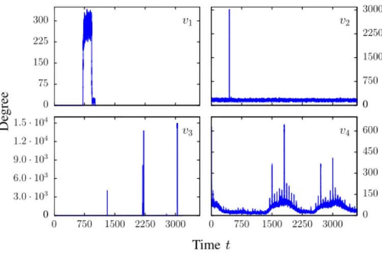
all outliers disappeared. Figure 10 shows the degree profiles of 4 nodes which have been removed for time periods during which they were acting abnormally.
VIII. VALIDATION
The IP traffic trace we use does not have a ground truth dataset listing abnormal IP addresses and instants. However, we can validate our results by looking at the consequences of the removals on the average degree per second.
Let dt be the instantaneous average degree at time
t: dt= V1 Pvdt(v). The average degree during second
si = [i, i + 1], denoted by d(si), is the average of dt from
t = i to t = i + 1, for all i ∈ {0, · · · , 3599}: d(si) =
Z i+1
i
d(t) dt .
We see in Figure 11.a that the average degree per second is homogeneously distributed with outliers. After removing events identified with our method, we see in Figure 11.b that peaks as well as sudden changes in the trend disappear, while the average over time stays unaltered. Likewise, in
0 75 150 225 300 v1 0 750 1500 2250 3000 v2 0 3.0 · 103 6.0 · 103 9.0 · 103 1.2 · 104 1.5 · 104 0 750 1500 2250 3000 v3 0 750 1500 2250 3000 0 150 300 450 600 v4 De gree Time t
Fig. 10:Degree profiles of four identified nodes - v1is responsible for outliers observed in C22= {252, ..., 2510}. The set {(t, v1) : t ∈
[712, 940[ and dt(v) ∈ C22} has been identified and removed. v2
has a normal activity with a degree around 160 and a sharp variation on T223= [446, 448[. The set {(t, v2) : t ∈ T223 and dt(v) ∈ C32}
has been identified and removed. Sets {(t, v3)} where v3 is active
have all been identified and removed. For node v4, the four peaks
corresponding to degree values higher than 300 have been identified and removed. The degree profiles of these nodes suggest that they
constitute malicious activity [22], [32]. Node v3 reaches several
powers of two indicating that it is running network scans. We observe
a similar behaviour around a degree of 256 for node v1.
a) Distribution of the average degree per second
Distrib ution 0 0.02 0.04 0.06 0.08 0.1 0.12 0.14 0 0.001 0.002 0.003 0.004
Average degree per second Before Removals
0.00025 0.0003 0.00035 0.0004 0.00045
Average degree per second After Removals
b) Time evolution of the average degree per second
A v erage de gree per sec. × 10 − 3 0 1.0 2.0 3.0 4.0 0 600 1200 1800 2400 3000 3600 Timet(seconds) Before Removals 0 600 1200 1800 2400 3000 3600 Timet(seconds) After Removals
Fig. 11:Consequences of event removals on the average degree per second - Our method succeeds in removing identified anomalies with no significant impact on the underlying normal traffic.
the distribution, all outliers disappear but the bell curve stays the same. Quantitatively, we find 33 outlying seconds before removals versus 5 after applying our method. The average over time of the average degree per second is equal
to 3.39571 · 10−4 before removals, and to 3.31795 · 10−4
after removals. These results show that our method succeeds in removing abnormal traffic without altering the underlying normal traffic.
These results highlight another important fact. An outlier in distribution of Figure 11.a means that there is a second during which the average degree is larger than usual. This event is detected but not identified since we cannot trace back responsible nodes with this aggregated feature. By using the instantaneous degree on couples (t, v), our method is able to identify events unidentified with the average degree per second. This last result is particularly promising: it shows that by using more complex and less aggregated features, it is possible to identify events previously detected but unidentified with simpler metrics. Then, the 195 events that we were not able to identify with the instantaneous degree of nodes could therefore be identified in future works by using other link stream features.
IX. OTHERDATASETS
To test the generality and applicability of our method, we test it on other datasets from the MAWI archive. In this section, we present the main results and differences we observe with these datasets.
A. One day long IP traffic trace from June 2013
We use here a one day long IP traffic capture from the MAWI archive from June 25th, 2013, at 00:00 to June 26th,
2013, at 00:00. The set D contains 2, 196, 079, 591 triplets involving 15, 390, 238 different IP addresses. This dataset is larger than the first one and covers one day of IP traffic with its circadian cycle. We keep identical time slices size and degree classes size.
Figure 12.a (left) shows, for C2 = {2}, the distribution on
all time slices Ti of the fraction fi(C2). Partly as a result of
circadian cycles, we see that this distribution consists of three normal distributions. To address this issue, we normalize the degree with the average degree per second and consider the normalized degree, denoted by dt(v), such that
dt(v) =
dt(v)
d(btc),
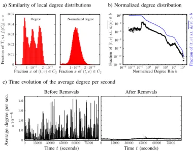
where btc, the floor function of t, is the second to which t belongs. We see in Figure 12.a (right) that local distributions on time slices are similar and in Figure 12.b that the global normalized degree distribution is heterogeneous. Thus, the two constraints required to apply our method are met. We find 34 degree classes, from C1 = {1} to C34 = {3982, . . . , 5011}.
Among these, 3 classes are rejected because they do not fit with an homogeneous distribution with outliers. We find 11
a) Similarity of local degree distributions
0 0.01 0.02 0.03 0.04 0.05 0 1 · 10−5 2 · 10−5 Fraction of Ti s.t fi (C 2 ) = x Fraction x of (t, v) ∈ C2 Degree 0 1 · 10−6 2 · 10−6 Fraction x of (t, v) ∈ C2 Normalized degree
b) Normalized degree distribution
10−12 10−10 10−8 10−6 10−4 10−2 100 10−610−410−2 100 102 104 106 108 Fraction of (t, v ) s.t. dt (v ) ∈ b Fraction of (t, v ) s.t. dt (v ) > b
Normalized Degree Bin b c) Time evolution of the average degree per second
A v erage de gree per sec. × 10 − 4 0 1.0 2.0 3.0 4.0 0 15000 30000 45000 60000 75000 Timet(seconds) Before Removals 0 15000 30000 45000 60000 75000 Timet(seconds) After Removals
Fig. 12: Results on a one day long IP traffic trace - After degree normalization, both the similarity of local distributions and the heterogeneity of the global distribution are verified. Results are validated by the average degree per second after removals in which the normal traffic is preserved. Note that in the global distribution (b), the normalized degree has been rescaled with a constant to have a better range of values and values are merged into bins to smooth the distribution.
AN -classes from k = 1 to k = 26 and 20 A-classes from k = 51 to k = 5011. We detect 22, 669 outliers and succeed in identifying 63% of them. To do so, we removed 8.7% of all the traffic. Once again, we see in Figure 12.c that these removals lead to the cleaning of the average degree per second: 1, 672 abnormal seconds before removals and 10 after. Likewise, normal traffic stays unchanged: the average over time of the average degree per second is equal to 1.53199 · 10−5 before removals and to 1.48824 · 10−5 after.
B. Fifteen-minute IP traffic trace from November 2018: com-parison to MAWILab
We use here a fifteen-minute IP traffic capture from the
MAWI archive on November 3rd, 2018, from 14:00 to 14:15.
The set D contains 64, 913, 871 triplets involving 16, 453, 608 different IP addresses. This dataset is more recent than the first one and has a list of anomalies indexed by MAWILab [17] to which we can compare our results. Given the shorter temporal extent, we take time slices of size τ = 1.0s instead of τ = 2.0s, in order to keep a significant number of time slices. Degree classes stay unchanged.
We observe an heterogeneous global degree distribution and similar local degree distributions on time slices of 1.0 seconds (see Figures 13.a and 13.b). We find 43 degree
classes, from C1 = {1} to C43 = {31623, . . . , 39810}.
Among these, there are 23 AN -classes, 17 A-classes and 3 R-classes.
Contrarily to previous datasets, we observe three AN
C27 = {795, . . . , 1001} and C40 = {15849, . . . , 19953}.
We can see in Figure 13.d, that this is due to three nodes which have a constant degree fluctuating within each of these classes and, as a result, form the observed normal traffic. In this dataset, several removals generated negative outliers. For instance, the removal of event (C40, T752)
generated a negative outlier in class C1. The
corresponding event was incorrectly identified by the
set I(C40, T752) = {(t, v) : t ∈ T752 and dt(v) ∈ C40}.
Indeed, this event corresponds to the spike of activity of node
v3 from 755.3 to 756.5 (see Figure 13.d). Yet, the normal
behaviour of v3 is to be linked to an average of 18, 178
nodes of degree 1 over time. Thus, the removal of its activity during this time period leads to a negative outlier in C1,
since, in addition to removing abnormal interactions of v3,
it also removes its legitimate interactions. This shows that to identify event (C40, T752), we need to use a finer and more
complex feature than the degree.
Finally, our method enabled us to detect 827 outliers and identify 796 of them (96%). To do so, we removed 1.2% of all the traffic. We see in Figure 13.c that, as with the two other datasets, removals lead to a traffic free of most degree-related anomalies. The number of abnormal seconds is equal to 19 before removals versus 0 after removals. Likewise, the average over time of the average degree per second goes from 9.311934 · 10−5 to 9.198076 · 10−5 after removals.
This dataset contains a MAWILab database to which we can compare our results [17]. It lists and labels anomalies in traffic from the MAWI archive by using a graph-based methodology that compares and combines the output of
several independent anomaly detectors. On November 3rd,
2018, from 14:00 to 14:15, it indicates a total of 287 anomalous IP addresses. To each of these is associated a time period during which it is evaluated as abnormal and a label classifying its anomaly type among the following categories [32]:
– Point to point denial of service: a large number of packets are sent between two IP addresses;
– Distributed denial of service: a large number of packets are sent between multiple sources and one destination;
– Network scan: an IP address scans a network of several destination IP addresses;
– Port scan: an IP address scans several ports of one destination;
– Point multipoint: normal router traffic; – Alpha flow: normal peer to peer traffic; – Other: normal outage traffic;
Since we do not consider the port number, and given that the degree feature does not account for the number of exchanged packets, anomalies within the point to point denial of service, port scan and alpha flows categories cannot be detected by our method. Moreover, we do not consider events corresponding
to legitimate traffic. This reduces the number of identified IP addresses to 77.
With our method, we find 33 anomalous IP addresses. Six of them are not listed by MAWILab. They correspond to node v2 in Figure 13.d and nodes v4, v5, v6, v7 and v8 in Figure
13.e (left). Node v2 has been removed during its spike of
activity from 798.18 to 799.87. Likewise, node v7 has been
removed from 814.06 to 815.00 and node v8 on the whole
time period during which it is active. Note that, as we can see in Figure 13.e (middle and right), nodes v7 and v8 activities
are typical of nodes performing network scans which are usually detected by MAWILab. The remaining three nodes v4, v5 and v6, have been removed on periods of respectively
0.0768s, 0.0677s and 0.181s because of their ephemeral activity within the A-class C22= {252, . . . , 317}. This could
be avoided by using larger classes (see section X-B). In the network scan category, we identified 24 IP addresses among the 76 (32.6%) listed by MAWILab. All network scans involving more than 250 different destinations have been identified with our method. As mentioned above, we identified in addition two IP addresses that the MAWILab detectors missed (see Figure 13.e). Moreover, for the corresponding events, our temporal precision is much better than the one provided by MAWILab detectors. However, our method fails to identify IP addresses permanently linked to the network since they have constant degree profiles and therefore lead to AN -classes. More generally, we did not find IP addresses which scan networks involving less than 250 destinations since all classes below C22 = {252, . . . , 317}
are AN -classes, and since their activities are not linked to the ones of removed events. Nonetheless, time slices during which most of these network scans occur have been detected as outliers in their corresponding degree class. This inability to identify low degree classes events could be avoided by using a feature different from the degree, in which the corresponding malicious activities deviate more significantly.
In the distributed denial of service category, only one anomaly is identified by MAWILab. The corresponding node have a maximum degree of 53. Hence, we do not find it with our method for the same reasons as above.
The six remaining nodes we identified fall in the point to multipoint category that we do not consider as it constitutes normal router traffic.
Finally, Figure 13.c (right) shows the average degree per second after removing events identified with our method as well as the ones identified in the MAWILab dataset. We see that, with MAWILab, the average over time is affected by the removals. This is mostly due to the poor time precision used by MAWILab to describe anomalies. Indeed, 63% of IP addresses are identified as abnormal on the whole trace, including IP addresses which have a global constant degree with only a few spikes. With our method, instead, when nodes
a) Global degree distribution 10−16 10−14 10−12 10−10 10−8 10−6 10−4 10−2 100 101 102 103 104 105 Fraction of (t, v ) s.t. dt (v ) = k Fraction of (t, v ) s.t. dt (v ) > k Degree k
b) Similarity of local degree distributions
0 0.01 0.02 0.03 0.04 0.05 0.06 0.07 −0.2 0 0.2 0.4 0.6 0.8 1 1.2 1.4 1.6 Fraction of (f i ,f j )i6= j RatioDi,j/c
c) Time evolution of the average degree per second
A v erage de gree per sec. × 10 − 4 0.6 0.8 1.0 1.2 1.4 1.6 0 100 200 300 400 500 600 700 800 900 Timet(seconds) Before Removals 0 100 200 300 400 500 600 700 800 900 Timet(seconds) After Removals MAWILab
d) Constant and high degree nodes
100 101 102 103 104 105 0 100 200 300 400 500 600 700 800 900 dt (vi ) t v1 v2 v3
e) Nodes undetected by MAWILab
0 100 200 300 400 500 600 700 800 0 100 200 300 400 500 600 700 800 900 dt (vi ) t C22 v4, v5, v6 v8 v7 0 50 100 150 200 250 300 0 100 200 300 400 500 600 700 800 900 t v7
MAWILab + our method Our method only
0 100 200 300 400 500 600 700 800 0 50 100 150 200 250 300 350 400 t v8
MAWILab + our method Our method only
Fig. 13:Fifteen minutes from November the 3rd 2018 - (a - b) The heterogeneity of the global degree distribution and the similarity of local degree distributions are verified. (c) Results are validated by the average degree per second after removals. Contrary to our method, we observe a decrease of the average over time when removing events identified by MAWILab. (d) AN -classes are observed in high degree classes: v1 is responsible for the normal traffic observed in C24= {399, . . . , 502}; v2 for the one in C27= {795, . . . , 1001} and v3for the one in C40= {15849, . . . , 19953}. (e) Nodes v2, v4, v5, v6, v7 and v8 are not detected by MAWILab. However, we see that the removal
of the abnormal activity of v2 is responsible for the disappearance of the spike around t = 800 in (c) and that v7 and v8have a suspicious
activity which is usually detected by MAWILab. Note that high degree node v3in (d) has been removed from the calculation in the average
degree per second in (c) to have a greater clarity.
have a constant degree, classes within which their degree fluctuates are labelled as AN -classes. Thus, their activities are not removed and normal traffic stays unchanged.
X. INFLUENCE OFPARAMETERS
We showed the efficiency of our method on several datasets. In this section, we perform a series of experiments on the first dataset to study the influence of parameters τ , for time slice duration, and r, for degree class size.
A. Variation of Time Slice Sizes
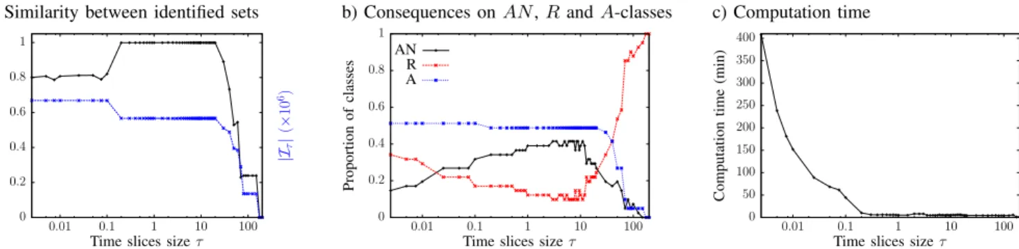
We divide the link stream into time slices of size τ in order to compare local degree distributions. The success of our method is based on the fact that they are similar from one time slice to another. Due to aggregation over a larger period, it is expected that the larger τ , the larger the similarity between time slices, and conversely when the size decreases. Let Iτ = ∪i,jI(Cj,Ti)be the set of identified outliers using
time slices of size τ . In order to evaluate the impact of τ , we measure the Jaccard similarity coefficient between I2.0,
obtained in the first experiment, and other sets obtained by varying τ :
J (I2.0, Iτ) =
|I2.0∩ Iτ|
|I2.0∪ Iτ|
.
Results are depicted in Figure 14.a. We see that identified sets Iτare identical from τ = 0.2 up to τ = 20.0. This shows that
our method is stable with respect to this parameter. Below this range, we are able to identify slightly more outliers. On the contrary, when the size increases, we identify less and less
outliers until no more is identified after τ = 175.0. This is explained by the number of AN , A and R-classes according to τ in Figure 14.b: the more τ increases, the higher the number of R-classes and the lower the number of A-classes in which we are able to identify events. When we reach τ = 175.0, all classes are rejected, hence no outlier is detected. This increase in the number of rejected classes is provoked by the very small number of time slices when τ gets larger. Indeed, time slices are insufficiently numerous to establish a normal behaviour and, for all classes C, fits between fractions fi(C) and a normal distribution are more likely to be rejected.
We identify more abnormal couples (t, v) when τ is small. However, this result should be taken with caution. As we can see in Figure 14.b, when τ decreases, the number of rejected classes increases and the number of AN -classes decreases. Indeed, the smaller the time slice, the less the behaviour between time slices is similar, which leads to a rejection of normal behaviour. A-classes are not affected: in most time slices, there is no node that reaches a degree within the class, whatever the time slice size. Moreover, their number increases. This is explained in Figure 15. We see that for τ = 0.25, there is 83% of Ti for which the fraction
fi(C34) is zero, against 67% for τ = 2.0. When τ decreases,
the proportion of time slices without traffic in the class compared to the ones that contain traffic is much higher than in experiments with a larger τ . If the increase of A-classes makes it possible to identify more outliers, the decrease of AN -classes, on the other hand, prevents us from determining if a removal is bad or not by the appearance of a negative
a) Similarity between identified sets 0 0.2 0.4 0.6 0.8 1 0.01 0.1 1 10 100 J (I2 .0 ,I τ ) |Iτ | (× 10 6)
Time slices size τ
b) Consequences on AN , R and A-classes
0 0.2 0.4 0.6 0.8 1 0.01 0.1 1 10 100 Proportion of classes
Time slices size τ AN R A c) Computation time 0 50 100 150 200 250 300 350 400 0.01 0.1 1 10 100 Computation time (min)
Time slices size τ
Fig. 14:Time slice size influence - (a) The Jaccard index between identified sets shows that our method is stable from τ = 0.2 to τ = 20.0. (b) Small time slices lead to an increase of the number of A and R-classes while large time slices lead to a high number of R-classes but small number of AN and A-classes. (c) The computation time significantly increases as τ decreases.
3400 3600 3800 4000 4200 1312 1313 1314 1315 1316 1317 1318 dt (u ) t C34 τ = 2.0 τ = 0.25 τ 0.25 2.0 Detected (C34, T5256), (C34, T5257) (C34, T657) outliers (C34, T5258), (C34, T5259) Identified {(t, v) : t ∈ [1314, 1315[ {(t, v) : t ∈ [1314, 1316[ outliers and dt(v) ∈ C34} and dt(v) ∈ C34}
Removal u from 1314.24 to 1314.95 u from 1314.24 to 1314.95
Fig. 15: Number of Aclasses and removals depending on τ
-Node u has abnormal traffic within degree class C34. In the sample,
there are 4 time slices with abnormal traffic out of 24 using τ = 0.25 and 1 time slice with abnormal traffic out of 3 using τ = 2.0. This influences the proportion of A-classes but not the temporal precision on which the outlier is removed: with τ = 0.25 (red dots), we remove
u from 1314.24 to 1314.25 (T5256), then from 1314.25 to 1314.75
(T5257,T5258), and finally from 1314.75 to 1314.95 (T5259). With τ = 0.25 (black triangles), we remove u from 1314.24 to 1314.95 (T657).
outlier. Hence, our validation criteria for removals cannot be applied which could lead to a disruption of normal traffic.
In addition, we see in Figure 14.c that using small time slices significantly increases computation time.
Finally, note that, thanks to the modelling of traffic as a link stream, the time slice size does not affect the temporal precision with which we identify events since the time period during which a node is within an A-class is the same whatever the considered time slice (see Figure 15).
B. Variations of the Degree Class Size
We divide local degree distributions into degree classes of size r. The success of our method is based on the fact that distributions of fractions fi(Cj) on all time slices Ti and
degree classes Cj are homogeneous.
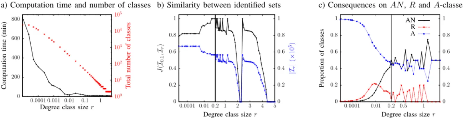
First notice that due to class construction, the total number of classes is very large when r is small and decreases rapidly when r increases (see Figure 16.a). For r = 10−5, there are 23, 983 classes; for r > 1.6, the total number of classes is smaller than 4 and reaches 1 for r > 4.4. Consequently, the smaller r, the higher the computation time.
When we look at the size and similarity of identified sets, we observe several phenomena (see Figure 16.b):
1) the number of identified outliers increases for r < 0.2; 2) we do not identify outliers for r ∈ [2.2, 2.3] and r > 4.4; 3) the Jaccard index is higher than 0.8 for r ∈ [10−5, 1.6] and r ∈ [2.4, 3.3];
4) the Jaccard index fluctuates between 0.8 and 1 for r ∈ [0.2, 1.6];
5) the number of identified outliers drops from r = 1.7, increases from r = 2.4, then drops again from r = 3.4. Once again, these observations are linked to the proportions of the three classes types. We explain them in detail in the following.
When the degree class size is too small, classes do not longer integrates degree fluctuations (see Figure 17). As we can see in Figure 16.c, this leads to an increase of A and R-classes at the expense of AN -classes which decrease. As above, while the increase of A-classes makes it possible to identify more outliers (observation 1), the decrease of AN -classes prevents us from using our validation criteria for removals which could lead to a disruption of normal traffic. On the contrary, when the degree class size is too large, classes integrate too much traffic. As a consequence, we can see in Figure 16.c, that the more r increases the more A-classes decreases. Therefore, the more r increases, the less we identify outliers. This is how we explain observation 2:
a) Computation time and number of classes 0 200 400 600 800 0.0001 0.001 0.01 0.1 1 10 0 101 102 103 104 105 Computation time (min) T otal number of classes
Degree class size r
b) Similarity between identified sets
0 0.2 0.4 0.6 0.8 1 0.01 0.2 0.0001 J (I0 .1 ,I r ) 1 2 3 4 50 0.2 0.4 0.6 0.8 1 |Ir | (× 10 5)
Degree class size r
c) Consequences on AN , R and A-classes
0 0.2 0.4 0.6 0.8 1 0.01 0.2 0.0001 Proportion of classes 0.5 1 0 0.2 0.4 0.6 0.8 1
Degree class size r AN
R A
Fig. 16:Degree classes size influence - (a) Due to the large number of classes, the computation time significantly increases as r decreases.
(b) The Jaccard index between identified sets shows that our method is stable from r = 10−5to r = 1.6. (c) Small degree classes lead to
an increase of the number of A-classes and to a decrease of the number of AN -classes. For r < 0.02, the proportion of R-classes is higher than the one of AN -classes. For r > 0.2, proportions of A and AN -classes are similar and the proportion of R-classes is low. Note that we did not plotted the proportion of classes for r > 1.4 because of fluctuations due to the small number of classes.
10000 15000 20000 25000 30000 0 100 200 300 400 500 600 700 800 900 dt (v ) t Class with r = 0.1 Classes with r = 0.01
Fig. 17: Consequences of small classes - When r = 0.01, classes are too small and do not contain fluctuations. As a consequence, for r = 0.01, we observe 6 AN -classes and 4 R-classes instead of only one AN -class for r = 0.1. Note that this node comes from the dataset of November 2018.
for r = 2.2, there are two AN -classes; for r = 2.3; there are one AN -class and one R-class; and finally, for r > 4.4, there is only one AN -class. Moreover, we see in Figure 18 that when class C1 contains several values of degrees, the
resulting distribution looks the same as when it only contains degree 1. Hence, the large proportion of couples (t, v) having degree 1 obstructs the traffic of couples (t, v) which have a degree larger than 1. As a consequence, we detect less outliers and incorrect removals could be accepted which could also lead to a disruption of normal traffic.
Finally, observations 3, 4 and 5 are explained by discretization effects. In the one-hour traffic trace, classes are arranged such that low degree classes are AN -classes and high degree classes are A-classes. Let kid be the smallest
degree from which we are able to identify events. As we can see in Figure 19, kid is different depending on the chosen r.
The smaller kid, the larger the number of detected outliers.
Until r = 0.2, kid is lower than 250 and the number of
0 0.01 0.02 0.03 0.04 0.0016 0.002 0.0024 0.0028 0.0032 Fraction of Ti s.t fi (C 1 ) = x Fraction x of (t, v) ∈ C1 r = 0.1 : C1= {1} 0 0.01 0.02 0.03 0.04 0.0016 0.002 0.0024 0.0028 0.0032 Fraction of Ti s.t fi (C 1 ) = x Fraction x of (t, v) ∈ C1 r = 0.5 : C1= {1, 2, 3} 0 0.01 0.02 0.03 0.04 0.0016 0.002 0.0024 0.0028 0.0032 Fraction of Ti s.t fi (C 1 ) = x Fraction x of (t, v) ∈ C1 r = 1.0 : C1= {1, · · · , 9} 0 0.01 0.02 0.03 0.04 0.0016 0.002 0.0024 0.0028 0.0032 Fraction of Ti s.t fi (C 1 ) = x Fraction x of (t, v) ∈ C1 r = 2.0 : C1= {1, · · · , 999}
Fig. 18:Class C1 depending on r - There are numerous couples
(t, v) which have degree 1: when C1 also contains degrees larger
than 1, we see no difference between the corresponding distributions. Therefore, for r > 0.3, we detect the same outliers as with r = 0.1, since outliers for which dt(v) > 1 are included within the Gaussian. Note that we zoomed on the Gaussian for greater clarity.
identified outliers is maximal. Then, kid fluctuates between
250 and 2, 512, which explain observation 4. A lot of outliers are located within this range. Hence, if kid ∈ [250, 2512],
these outliers are identified, otherwise they are not, which explains observation 3. Regarding observation 5, this is what happens: for r ∈ [1.7, 2.1], the number of classes is equal to three. There are two AN -classes and one A-class. The smallest degree of identification kid increases with r which
causes the drop in the number of identified outliers. For r ∈ [2.2, 4.3], the total number of classes is two. The number of detected outliers depends on classes proportions: there are either two AN -classes (r = 2.2), or one AN -class and one R-class (r = 2.3), or one AN -class and one A-class (r ∈ [2.4, 4.3]). Finally, we observe the same phenomenon,
for r ∈ [2.4, 4.3], kid increases with r which causes the
drop of the number of identified outliers until only one class remains for r > 4.3.
250 2512 5000 7500 10000 12500 15000 17500 20000 0 0.5 1 1.5 2 2.5 3 3.5 4 4.5 5 Smallest de gree of identification kid
Degree class size r
Fig. 19:Smallest degree of identification according to r - When
kid ∈ [250, 2512], the Jaccard index is higher than 0.8. However,
when kid > 2512, the number of identified outliers drops (dashed
red line) and reaches 0 in shaded zones.
The method instability with respect to r is only observed for a number of classes lower than 4 (r > 1.6). For a number of classes ranging from 24, 000 (r = 10−5) to 4, the method is stable and exhibits very similar results. Therefore, r must be chosen based on data range, by keeping a reasonably high number of classes.
XI. CONCLUSION
When dealing with IP traffic, we are faced with IP addresses having very different behaviours. In this context, one question arises: how to differentiate normal behaviours from abnormal ones. In this paper, we proposed a solution to this issue. We introduced a method that detects outliers in IP traffic modelled as a link stream by studying the degree of node over time. We applied our method on three datasets from the MAWI archive: one-hour long IP traffic trace from June 2013, one-day long IP traffic trace from June 2013 and a fifteen-minute long IP traffic trace from November 2018. Likewise, we performed series of experiments by varying the parameters used. In all these situations, we obtained stable results pointing interesting anomalous activities in IP traffic, independently of the degree order of magnitude. Moreover, we surgically removed anomalous traffic, which allowed us to validate our identification, identify more subtle outliers and recover a normal traffic with respect to the degree feature. This work however is only a first step towards anomaly detec-tion in link streams and may be improved on several aspects. We could extend our method with more complex features than the degree in order to find more complex anomalies and to identify the remaining events unidentified with the degree. This task would be simplified by the fact that largest anomalies have already been removed from the remaining traffic, allowing for a more detailed and finer analysis. At broader scale, our work could be useful in the field of IP traffic modelling as we would be able to generate normal traffic according to a specific feature. Likewise, thanks to
their individual extraction, anomalies could also be studied separately for a better characterization.
ACKNOWLEDGEMENT
This work is funded in part by the European Commission H2020 FETPROACT 2016-2017 program under grant 732942 (ODYCCEUS), by the ANR (French National Agency of Research) under grants ANR-15- E38-0001 (AlgoDiv), by the Ile-de-France Region and its program FUI21 under grant 16010629 (iTRAC).
REFERENCES
[1] B. L. Agarwal. Basic statistics. New Age International, 2006. [2] C. Aggarwal. Outlier Analysis. Springer International Publishing, 2016. [3] L. Akoglu and C. Faloutsos. Event detection in time series of mobile communication graphs. In Army science conference, pages 77–79, 2010. [4] L. Akoglu, H. Tong, and D. Koutra. Graph based anomaly detection and description: a survey. Data mining and knowledge discovery, 29(3):626– 688, 2015.
[5] M. Araujo, S. Papadimitriou, S. G¨unnemann, C. Faloutsos, P. Basu, A. Swami, E. E. Papalexakis, and D. Koutra. Com2: fast automatic dis-covery of temporal (‘comet’) communities. In Pacific-Asia Conference on Knowledge Discovery and Data Mining, pages 271–283. Springer, 2014.
[6] H. Asai, K. Fukuda, P. Abry, P. Borgnat, and H. Esaki. Network application profiling with traffic causality graphs. International Journal of Network Management, 24(4):289–303, 2014.
[7] P. Barford, J. Kline, D. Plonka, and A. Ron. A signal analysis of network traffic anomalies. In Proceedings of the 2nd ACM SIGCOMM Workshop on Internet measurment, pages 71–82. ACM, 2002.
[8] V. Batagelj and S. Praprotnik. An algebraic approach to temporal network analysis based on temporal quantities. Social Network Analysis and Mining, 6(1):28, 2016.
[9] M. Berlingerio, D. Koutra, T. Eliassi-Rad, and C. Faloutsos. Netsimile: A scalable approach to size-independent network similarity. arXiv preprint arXiv:1209.2684, 2012.
[10] P. Borgnat, G. Dewaele, K. Fukuda, P. Abry, and K. Cho. Seven years and one day: Sketching the evolution of internet traffic. In INFOCOM 2009, IEEE, pages 711–719. IEEE, 2009.
[11] A. Casteigts, P. Flocchini, W. Quattrociocchi, and N. Santoro. Time-varying graphs and dynamic networks. International Journal of Parallel, Emergent and Distributed Systems, 27(5):387–408, 2012.
[12] D. Chakrabarti. Autopart: Parameter-free graph partitioning and outlier detection. In European Conference on Principles of Data Mining and Knowledge Discovery, pages 112–124. Springer, 2004.
[13] V. Chandola, A. Banerjee, and V. Kumar. Anomaly detection: A survey. ACM computing surveys (CSUR), 41(3):15, 2009.
[14] Z. Chen, W. Hendrix, and N. F. Samatova. Community-based anomaly detection in evolutionary networks. Journal of Intelligent Information Systems, 39(1):59–85, 2012.
[15] D. Duan, Y. Li, Y. Jin, and Z. Lu. Community mining on dynamic weighted directed graphs. In Proceedings of the 1st ACM international workshop on Complex networks meet information & knowledge man-agement, pages 11–18. ACM, 2009.
[16] D. Eswaran and C. Faloutsos. Sedanspot: Detecting anomalies in edge streams. ICDM. IEEE, 2018.
[17] R. Fontugne, P. Borgnat, P. Abry, and K. Fukuda. Mawilab: com-bining diverse anomaly detectors for automated anomaly labeling and performance benchmarking. In Proceedings of the 6th International COnference, page 8. ACM, 2010.
[18] F. E. Grubbs. Procedures for detecting outlying observations in samples. Technometrics, 11(1):1–21, 1969.
[19] M. Gupta, J. Gao, Y. Sun, and J. Han. Community trend outlier detection using soft temporal pattern mining. In Joint European Conference on Machine Learning and Knowledge Discovery in Databases, pages 692– 708. Springer, 2012.
[20] M. Gupta, J. Gao, Y. Sun, and J. Han. Integrating community matching and outlier detection for mining evolutionary community outliers. In Proceedings of the 18th ACM SIGKDD international conference on Knowledge discovery and data mining, pages 859–867. ACM, 2012.
[21] J. Han, J. Pei, and M. Kamber. Data mining: concepts and techniques. Elsevier, 2011.
[22] H. Huang, H. Al-Azzawi, and H. Brani. Network traffic anomaly detection. arXiv preprint arXiv:1402.0856, 2014.
[23] T. Id´e and H. Kashima. Eigenspace-based anomaly detection in com-puter systems. In Proceedings of the tenth ACM SIGKDD international conference on Knowledge discovery and data mining, pages 440–449. ACM, 2004.
[24] K. Ishibashi, T. Kondoh, S. Harada, T. Mori, R. Kawahara, and S. Asano. Detecting anomalous traffic using communication graphs. In Telecom-munications: The Infrastructure for the 21st Century (WTC), 2010, pages 1–6. VDE, 2010.
[25] A. Kato, J. Murai, S. Katsuno, and T. Asami. An internet traffic data repository: The architecture and the design policy. In INET’99 Proceedings, 1999.
[26] A. Lakhina, M. Crovella, and C. Diot. Diagnosing network-wide traffic anomalies. In ACM SIGCOMM Computer Communication Review, volume 34, pages 219–230. ACM, 2004.
[27] M. Latapy, A. Hamzaoui, and C. Magnien. Detecting events in the dynamics of ego-centred measurements of the internet topology. Journal of Complex Networks, 2(1):38–59, 2013.
[28] M. Latapy, T. Viard, and C. Magnien. Stream graphs and link streams for the modeling of interactions over time. arXiv preprint arXiv:1710.04073, 2017.
[29] W. Lee, S. J. Stolfo, et al. Data mining approaches for intrusion detection. In USENIX Security Symposium, pages 79–93. San Antonio, TX, 1998.
[30] Y. L´eo, C. Crespelle, and E. Fleury. Non-altering time scales for aggregation of dynamic networks into series of graphs. Computer Networks, 148:108–119, 2019.
[31] E. Manzoor, S. M. Milajerdi, and L. Akoglu. Fast memory-efficient anomaly detection in streaming heterogeneous graphs. In Proceedings of the 22nd ACM SIGKDD International Conference on Knowledge Discovery and Data Mining, pages 1035–1044. ACM, 2016.
[32] J. Mazel, R. Fontugne, and K. Fukuda. A taxonomy of anomalies in backbone network traffic. In Wireless Communications and Mobile Computing Conference (IWCMC), 2014 International, pages 30–36. IEEE, 2014.
[33] M. Mongiovi, P. Bogdanov, R. Ranca, E. E. Papalexakis, C. Faloutsos, and A. K. Singh. Netspot: Spotting significant anomalous regions on dynamic networks. In Proceedings of the 2013 SIAM International Conference on Data Mining, pages 28–36. SIAM, 2013.
[34] H. J. Motulsky and R. E. Brown. Detecting outliers when fitting data with nonlinear regression–a new method based on robust nonlinear regression and the false discovery rate. BMC bioinformatics, 7(1):123, 2006.
[35] P. Papadimitriou, A. Dasdan, and H. Garcia-Molina. Web graph similarity for anomaly detection. Journal of Internet Services and Applications, 1(1):19–30, 2010.
[36] B. Pincombe. Anomaly detection in time series of graphs using arma processes. Asor Bulletin, 24(4):2, 2005.
[37] W. H. Press, S. A. Teukolsky, W. T. Vetterling, and B. P. Flannery. Numerical recipes in c: The art of scientific computing. second edition, 1992.
[38] S. Ranshous, S. Harenberg, K. Sharma, and N. F. Samatova. A scalable approach for outlier detection in edge streams using sketch-based approximations. In Proceedings of the 2016 SIAM International Conference on Data Mining, pages 189–197. SIAM, 2016.
[39] S. Ranshous, S. Shen, D. Koutra, S. Harenberg, C. Faloutsos, and N. F. Samatova. Anomaly detection in dynamic networks: a survey. Wiley Interdisciplinary Reviews: Computational Statistics, 7(3):223–247, 2015.
[40] H. Ringberg, A. Soule, J. Rexford, and C. Diot. Sensitivity of pca for traffic anomaly detection. ACM SIGMETRICS Performance Evaluation Review, 35(1):109–120, 2007.
[41] R. Saxena, S. Kaur, D. Dash, and V. Bhatnagar. Leveraging structural hierarchy for scalable network comparison. In International Conference on Database and Expert Systems Applications, pages 287–302. Springer, 2016.
[42] T. A. Schieber, L. Carpi, A. D´ıaz-Guilera, P. M. Pardalos, C. Masoller, and M. G. Ravetti. Quantification of network structural dissimilarities. Nature communications, 8:13928, 2017.
[43] J. Sun, C. Faloutsos, S. Papadimitriou, and P. S. Yu. Graphscope: parameter-free mining of large time-evolving graphs. In Proceedings
of the 13th ACM SIGKDD international conference on Knowledge discovery and data mining, pages 687–696. ACM, 2007.
[44] T. Viard, R. Fournier-S’niehotta, C. Magnien, and M. Latapy. Discover-ing patterns of interest in ip traffic usDiscover-ing cliques in bipartite link streams. In Proceedings of the International Conference on Complex Networks (CompleNet), 2018, 2018.
[45] Y. Virkar and A. Clauset. Power-law distributions in binned empirical data. The Annals of Applied Statistics, pages 89–119, 2014.
[46] K. Wehmuth, A. Ziviani, and E. Fleury. A unifying model for repre-senting time-varying graphs. In Data Science and Advanced Analytics (DSAA), 2015. 36678 2015. IEEE International Conference on, pages 1–10. IEEE, 2015.
[47] J. Whitbeck, M. Dias de Amorim, V. Conan, and J.-L. Guillaume. Temporal reachability graphs. In Proceedings of the 18th annual international conference on Mobile computing and networking, pages 377–388. ACM, 2012.
[48] N. Williams, S. Zander, and G. Armitage. A preliminary performance comparison of five machine learning algorithms for practical ip traffic flow classification. ACM SIGCOMM Computer Communication Review, 36(5):5–16, 2006.
[49] A. Wilmet, T. Viard, M. Latapy, and R. Lamarche-Perrin. Degree-based outliers detection within ip traffic modelled as a link stream. In 2018 Network Traffic Measurement and Analysis Conference (TMA), pages 1–8. IEEE, 2018.
[50] K. Xu, F. Wang, and L. Gu. Behavior analysis of internet traffic via bipartite graphs and one-mode projections. IEEE/ACM Transactions on Networking, 22:931–942, 2014.
[51] W. Yu, C. C. Aggarwal, S. Ma, and H. Wang. On anomalous hotspot discovery in graph streams. In Data Mining (ICDM), 2013 IEEE 13th International Conference on, pages 1271–1276. IEEE, 2013.


![Fig. 19: Smallest degree of identification according to r - When k id ∈ [250, 2512], the Jaccard index is higher than 0.8](https://thumb-eu.123doks.com/thumbv2/123doknet/13313936.399100/14.918.96.405.115.333/fig-smallest-degree-identification-according-jaccard-index-higher.webp)
