Boundary layer structure and decoupling from synoptic scale flow during NAMBLEX

HAL Id: hal-00301451

https://hal.archives-ouvertes.fr/hal-00301451

HAL is a multi-disciplinary open access

archive for the deposit and dissemination of sci-entific research documents, whether they are pub-lished or not. The documents may come from teaching and research institutions in France or abroad, or from public or private research centers.

L’archive ouverte pluridisciplinaire HAL, est destinée au dépôt et à la diffusion de documents scientifiques de niveau recherche, publiés ou non, émanant des établissements d’enseignement et de recherche français ou étrangers, des laboratoires publics ou privés.

Boundary layer structure and decoupling from synoptic

scale flow during NAMBLEX

E. G. Norton, G. Vaughan, J. Methven, H. Coe, B. Brooks, M. Gallagher, I.

Longley

To cite this version:

E. G. Norton, G. Vaughan, J. Methven, H. Coe, B. Brooks, et al.. Boundary layer structure and decou-pling from synoptic scale flow during NAMBLEX. Atmospheric Chemistry and Physics Discussions, European Geosciences Union, 2005, 5 (3), pp.3191-3223. �hal-00301451�

ACPD

Full Screen / Esc

Print Version

Interactive Discussion

EGU Atmos. Chem. Phys. Discuss., 5, 3191–3223, 2005

www.atmos-chem-phys.org/acpd/5/3191/ SRef-ID: 1680-7375/acpd/2005-5-3191 European Geosciences Union

Atmospheric Chemistry and Physics Discussions

Boundary layer structure and decoupling

from synoptic scale flow during

NAMBLEX

E. G. Norton1, G. Vaughan1, J. Methven2, H. Coe1, B. Brooks3, M. Gallagher1, and I. Longley1

1

School of Earth, Atmospheric and Environmental science, University of Manchester, Building Sackville Street, Manchester, M60 1QD, UK

2

Department of Meteorology, University of Reading, PO Box 243, Earley Gate, Reading, RG6 6BB, UK

3

School of the Environment, University of Leeds, Leeds, LSJ 9JT, UK

Received: 21 March 2005 – Accepted: 20 April 2005 – Published: 23 May 2005 Correspondence to: E. G. Norton (emily.norton@manchester.ac.uk)

ACPD

Full Screen / Esc

Print Version

Interactive Discussion

EGU

Abstract

This paper presents an overview of the meteorology and planetary boundary layer structure observed during the NAMBLEX field campaign to aid interpretation of the chemical and aerosol measurements. The campaign has been separated into five pe-riods corresponding to the prevailing synoptic condition. Comparisons between

meteo-5

rological measurements (UHF wind profiler, Doppler sodar, sonic aneometers mounted on a tower at varying heights and a standard anemometer) and the ECMWF analysis at 10 m and 1100 m identified days when the internal boundary layer was decoupled from the synoptic flow aloft. Generally the agreement was remarkably good apart from during period one and on a few days during period four when the diurnal swing in wind

10

direction implies a sea/land breeze circulation near the surface. During these periods the origin of air sampled at Mace Head would not be accurately represented by back trajectories following the winds resolved in ECMWF analyses. The wind profiler ob-servations give a detailed record of boundary layer structure including an indication of its depth, average wind speed and direction. Turbulence statistics have been used

15

to assess the height to which the developing internal boundary layer, caused by the increased surface drag at the coast, reaches the sampling location under a wide range of marine conditions. Sampling conducted below around 10 m will be impacted by emission sources at the shoreline in all wind directions and tidal conditions, whereas sampling above 15 m is unlikely to be affected in any of the wind directions and tidal

20

heights sampled during the experiment.

1. Introduction

The North Atlantic Marine Boundary Layer EXperiment (NAMBLEX) took place be-tween 1 August and 1 September 2002 at the Mace Head atmospheric research station (53.32◦N, 9.90◦W) on the west coast of Ireland.

25

considera-ACPD

Full Screen / Esc

Print Version

Interactive Discussion

EGU tions if measurements near the ground at Mace Head are to be related to long range

transport and the influence of distant surface emissions or air entrained into the bound-ary layer from the free troposphere. Also it is important, especially for short-lived con-stituents, to know if an internal boundary layer develops during periods of onshore flow which partially shelters the site from marine boundary layer air off the open ocean. The

5

main aims of NAMBLEX were to study oxidation chemistry, including that of halogens, in the marine boundary layer. As described elsewhere in this volume, a range of chem-ical and aerosol measurements were made at Mace Head, and on aircraft flights in the vicinity of the site (Heard, 20051). In addition, several meteorological instruments were deployed during the campaign, including sonic anemometers mounted on a tower at

10

heights between 7 and 24 m, a standard anemometer at 21 m, a UHF (1290 MHz) wind profiler and a Doppler sodar. In this paper we present a synthesis of the surface mea-surements with the UHF radar and large-scale synoptic fields, so that the chemical and aerosol measurements can be placed in a meteorological context. Of particular interest to the aims of this paper are to highlight periods when the local winds were decoupled

15

from the synoptic flow. In such conditions trajectory calculations used to deduce air mass origins are unreliable, so the interpretation of the chemical measurements must proceed with caution.

This paper will first describe the specialist meteorological instrumentation used at Mace Head. We then present an overall meteorological summary of the NAMBLEX

20

campaign, dividing it into five broad periods of similar synoptic type. Within each pe-riod, we present a time series of measurements from the various instruments and compare them to ECMWF analysis fields, to determine how well the analyses repre-sented the local conditions. This in turn is a measure of the reliability of trajectory calculations based on ECMWF data. Subsequently, we concentrate on measurements

25

of boundary-layer structure made by the UHF wind profiler, which show how

repre-1

Heard, D.: The North Atlantic Marine Boundary Layer Experiment, Overview of the cam-paign held at Mace Head, Ireland, in summer 2002, Atmos. Chem. Phys. Discuss., to be submitted, 2005.

ACPD

Full Screen / Esc

Print Version

Interactive Discussion

EGU sentative the surface measurements were of the boundary layer as a whole. Finally

turbulence statistics from the sonic anemometers are presented to asses the develop-ment of an internal layer.

2. Instrumentation

2.1. UHF wind profiler

5

‘Clear-air’ radars detect small scale irregularities in backscattered signals due to re-fractive index inhomogeneities caused by turbulence C2_n; (Doviak and Zrnic, 1993). In the lower troposphere such inhomogeneities are mainly produced by humidity fluc-tuations. ‘Clear-air’ Doppler shifts provide a direct measurement of the mean radial velocity along the radar beam. UHF radars also observe strong echoes from

precipita-10

tion which can be distinguished from the ‘clear-air’ echo by their intensity and spectral width.

The University Facility for Atmospheric Measurements (UFAM) mobile wind profiler is a ‘clear-air’ UHF Doppler radar system designed by Degreane Horizon to measure three components of wind 24 h a day under all weather conditions. The radar operates

15

at 1290 MHz (23 cm) with a peak power of 3.5 kW and beam width of 8.5◦. The radar consists of three panels that emit and receive three separate beams, each panel being an array of 64 dipole antennas. The vertical beam measures the vertical component of the wind and the two beams at an elevation of 73◦and orthogonal azimuths sample radial velocities that have contributions from both vertical and horizontal wind

compo-20

nents, to enable full wind vectors to be calculated. The radar provides measurements of wind speed and direction to an intrinsic accuracy of <1 ms−1 and <10◦respectively according to the manufacturer’s estimates.

The radar was cycled between measurements in two modes: the ‘low mode’ with a Gaussian shaped pulse of length 500 ns, inter-pulse period of 50 µs, average power

25

ACPD

Full Screen / Esc

Print Version

Interactive Discussion

EGU of length 1000 ns, inter-pulse period of 40 µs, average power of 100 W and duty cycle

of 2.5%. The vertical resolution was 75 m for the ‘low mode’ and 150 m for the ‘high mode’ up to altitudes of approximately 1500 m and 4000 m respectively depending on atmospheric conditions. The minimum altitude was 75 m, although in practice it was found to be in the region of 200 m due to ground clutter echoes. The characteristics of

5

the UFAM mobile wind profiler are summarized in Table1.

Echoes from the three beams at each altitude were combined and both temporal and vertical windowing was used to distinguish the ‘clear-air’ signal from any ground clutter or other interference. The wind profiler was located outside the top cottage 30 m above sea level and approximately 300 m from the shoreline. Measurements were derived

10

every 15 min using consensus averaging over 30 min around the nominal observation time. The radar was operational 24 h a day under all weather conditions for the duration of the campaign apart from when a timing fault on the transmit-receive switch caused the limiter to fail. This resulted in no wind profiler data between the 15 and 21 August. 2.2. Surface layer flux measurements

15

Four 3-axis sonic anemometers (R. M. Young Model 81000) were mounted on 2 m long booms at 7, 10, 15 and 24 m above the surface on the south-western corner of an open scaffold tower of footprint 1×2 m. The ground on which the tower stood was around 7 m above the sea surface at mid-tide heights and was approximately 50 m from the shoreline. The ground fell away close to the tower and a mixed rocky foreshore

20

extended to the ocean. In the easterly direction, the surface, composed mostly of rough grass and boulders, rose steadily over a distance of approximately 200 m. The wind speeds in the u, v and w co-ordinates were recorded every 0.05 s, providing 10 Hz response and turbulence statistics as a function of height above the surface.

ACPD

Full Screen / Esc

Print Version

Interactive Discussion

EGU 2.3. Sodar

The UFAM Doppler Sodar (SOnic Detection And Ranging) used during NAMBLEX was a Scintec MFAS64: a monostatic phased array system with 64 transmit and 64 receive transducers generating acoustic signals in the frequency range 1650 to 2750 Hz. The phased array allows for both the transmitted and the received signals to be steered to

5

reduce side lobe interference. Table2gives the detailed technical specifications of the system.

In a monostatic sodar system only the backscattered signal is detected. The intensity of the returned energy is proportional to the C2_T function, which, in turn, is related to the thermal structure and stability of the atmosphere. C2_T has characteristic patterns during

10

ground-based radiation inversions, within elevated inversion layers, at the periphery of convective columns or thermals, in sea breeze/land breeze frontal boundaries, and at any interface between air masses of different temperatures. The acoustic scattering is determined by Bragg scattering laws and only inhomogenities of the order of 1/2 the acoustic wavelength (5–10 cm) contribute. Using Doppler methods a measure of air

15

movement at the position of the scattering eddy can be determined.

In this application ten frequencies were used (Table 3) with longer pulse lengths at the lower frequencies to increase measurement range and shorter pulses at higher frequencies to increase height resolution. The acoustic beam was steered around four reference directions in turn (N, E, S, W) with a pulse sequence as described in Table3;

20

alternate pulses were directed either side of the reference direction.

The same pulse sequence was repeated 10 times for a given reference direction and the data averaged over 10 min. Due to the proximity of housing to the research site the operation of the sodar was restricted to the hours of 09:00 to 17:00 local time. During rain events the sodar output was reduced to zero due to scattering of the acoustic

25

ACPD

Full Screen / Esc

Print Version

Interactive Discussion

EGU

3. Meteorological summary

This meteorological summary for the NAMBLEX period has been compiled from syn-optic charts published by Weather for 12:00 GMT and the European Meteorological Bulletin for 00:00 GMT, along with meteorological measurements made at Mace Head. The daily maximum temperature over the campaign period remained in the range 12–

5

17◦C except for a warm spell between 1 and 6 August when the temperature was 16– 20◦C, with a warm spike on the 2 August (up to 24◦C). Prevailing synoptic conditions were used to separate the campaign into five periods:

1) 1 August to 5 August was complex, with the Azores high extending over the Atlantic and a stagnant low pressure system over Ireland and the UK, with

re-10

circulating fronts. Winds were very weak north-easterly from 1 to 5 August. 2) The Azores high extended towards Ireland and therefore winds were generally

westerly or north-westerly from 6 to 11 August, apart from the 8th when the centre of a depression crossed just south of Mace Head.

3) From 12 to 17 August the Azores high retreated south allowing a succession of

15

depressions to cross Ireland from the west.

4) On 18 August the air stagnated as the pressure gradually built. Anti-cyclonic conditions prevailed between 19 and 27 August.

5) The 28 to 31 August saw a return to westerlies and unsettled weather.

4. Comparison between wind speed and direction measurements and

meteoro-20

logical analysis

In order to interpret the chemical measurements at Mace Head it is necessary to sep-arate local and long-range contributions to the air sampled. This will be done by com-paring the local wind measurements to those in the corresponding ECMWF analyses,

ACPD

Full Screen / Esc

Print Version

Interactive Discussion

EGU and examining the consistency between surface winds and the flow aloft. We present

comparisons of wind speed and direction for two altitude regions: at low level between the 7 m, 10 m, 15 m and 24 m sonic anemometers, a standard anemometer at 21 m and ECMWF analyses at 10 m; and near the top of the boundary layer between the wind profiler at 1100 m and ECMWF analyses at 1100 m. Sodar data at 100 m was also

5

included in the comparisons for periods four and five. In the plots that follow night-time is indicated as the bold black line on the time axis.

4.1. Meteorological period one

Period one was the most complex meteorologically: local circulation effects dominated and a decoupled lower and upper boundary layer were observed. This is evident in the

10

comparison between 1 and 6 August of the wind direction versus time (Fig.1). The 1100 m winds from the radar (blue triangles) were from the north-eastern quadrant and agree with the ECMWF data (blue line) up to the afternoon of the 4th. A sharp veer of 90◦in wind direction observed by the radar around 12 h on the 5th was represented as a much more gradual change in the model with the winds rotating by 270◦ over 24 h.

15

Since this was a period of very low wind speed (<2 m s−1), the discrepancy between the two curves is much less significant than it appears.

The lower level winds were much more variable with a general tendency to be from the north-western quadrant. This variability was not represented in the ECMWF model winds which were generally northerly. During land breeze events the lower winds were

20

measured to be more easterly. This is clear on the night of the 2nd, 4th and 5th when the wind direction switched to be more easterly than the model during the night. The opposite occurred a few hours after dawn when the direction shifted more westerly than the ECMWF model. This is a characteristic sea breeze pattern. Close agreement in the wind directions was observed between the sonics positioned at different heights

25

on the tower. Period one was characterised by low wind speeds with a local circulation being the dominant influence on the ground based chemical measurements.

ACPD

Full Screen / Esc

Print Version

Interactive Discussion

EGU ECMWF analyses at 1100 m agree to within <2 ms−1apart from the night of the 4th. At

the lower levels wind speeds were very variable on 1st and 2nd, then settled into a sea breeze pattern with minimum speeds in early morning and maxima in late afternoon. The sea breeze circulation was not represented in the ECMWF model which bears little resemblance to the lower-level winds. These comparisons confirm that period one

5

was dominated by local flow introducing a high degree of error to trajectory calculations based on the ECMWF model. Indeed there are occasions in Fig.1 where the sonic anemometers at 10 m (red line) and 24 m (green line) on the tower show wind speeds that differ by up to to 2.0 ms−1, emphasising that chemical measurements at different altitudes during this period cannot be assumed to share a common source region.

10

4.2. Meteorological period two

This pattern of sea and land breezes disappeared on the morning of 6 August after the passage of an occluded front. Hence period two was defined between 6 and 11 August. During this period the wind direction was generally westerly to north-westerly, apart from the 8th when the centre of a depression passed just south of Mace Head.

15

During the passage of the depression the wind direction went full circle in an anti-clockwise direction from northwesterly to northerly.

The comparison for period two shows the wind direction measurements for the lower and upper levels tracking each other closely (Fig. 2). Excellent agreement was ob-served between the measurements and the ECMWF model analysis; a brief exception

20

to this rule occurred on the night of the 10th when the wind speed dropped to <2 ms−1 and hence local circulation effects dominated. For most of this period the wind speeds at 1100 m were similar to those near the ground with a systematic clockwise turning of the wind with height as expected from the Ekman spiral. Wind speeds at the two levels were also similar. Interestingly this agreement is not exhibited by the ECMWF

analy-25

ses, where winds are almost always stronger at the higher level. The model also fails to capture the variability of the measured winds, suggesting that some local influences

ACPD

Full Screen / Esc

Print Version

Interactive Discussion

EGU were present during this period. Nevertheless, the good agreement in wind direction

and overall average correctness of the speeds suggests that the ECMWF trajectory calculations should be fairly reliable during this period.

4.3. Meteorological period three

Another depression and occluded front passed over Mace Head on the evening of the

5

10th and early hours of the 11th. After the depression passed, a north-westerly airflow ensued and a ridge of high pressure started to develop, defining period three. Dur-ing this period three frontal systems passed over Mace Head, with the wind direction retaining a westerly component throughout (Fig. 3). As in period two the measured wind directions at the upper and lower levels were almost identical, with the ECMWF

10

model in close agreement. An exception was observed during the night/morning of the 13th/14th when the lower level wind vector rotated through the west. This was accompanied by very low wind speeds <2 ms−1. This time however the model and measurements also agree on wind speed (Fig.3), with both showing winds approxi-mately 5 ms−1 stronger at the upper level than the lower level. We therefore conclude

15

that trajectory calculations should be valid during this period. 4.4. Meteorological period four

After the passage of a warm and a cold front on the 17th the wind speed dropped off and anti-cyclonic conditions set in, with the direction remaining generally westerly (Fig.4). Radar data were only available from the 22nd on and agree very well with the

20

ECMWF model direction. The ECMWF analyses seem to capture a weak representa-tion of the sea breeze from the 18th to 20th, seen in the low level wind direcrepresenta-tion and speed (Fig.4). A sea breeze also occurred on the 25th.

The radar data from the 22nd onwards measured almost identical wind directions to the low-level instruments. Sodar measurements at 100 m (red crosses), available

25

ACPD

Full Screen / Esc

Print Version

Interactive Discussion

EGU direction. Agreement with the model wind speeds is generally good at both levels apart

from the sea breeze events. Trajectory calculations, outside of the sea breeze periods, should be reliable during this period.

4.5. Meteorological period five

Radar data ceased on the 30th and the anemometers and sodar data on 1 September

5

as the campaign ended. This westerly period was very similar to period two, with excellent agreement in wind direction between all the measurements and the ECMWF model and little directional wind shear in the boundary layer as shown by Fig.5. At both levels the wind speeds showed good agreement as shown by Fig. 5 indicating that trajectory calculations should be reliable during this period.

10

4.6. Comparison statistics

In summary, during the majority of the campaign good agreement was observed be-tween the meteorological measurements and the ECMWF model analysis. The major discrepancies were found at the lower altitudes during the sea breeze events that oc-curred in period one and also between 17 and 22 August and 25 August. Hence outside

15

the sea breeze events trajectory calculations based on ECMWF model analysis should be reliable. Comparison statistics between the ECMWF model and the wind profiler data were calculated for the whole measurement period at 1100 m. Comparisons with the sonic anemometer at 10 m has only been made during periods when sea breeze events were absent. The values of the correlation coefficients (r), root mean squared

20

residual (RMS), slope and slope error at 1100 m and 10 m are given for the wind speed, zonal velocity (u) and meridional velocity (v) in Table4. Correlation coefficients at the upper level gave an average value of r=0.940 and at the lower level an average value of r=0.898 confirming that outside the sea breeze events at the lower altitudes the ECMWF six hour model analysis of wind speed and direction were reliable. The slopes

25

ACPD

Full Screen / Esc

Print Version

Interactive Discussion

EGU detectable systematic offset between the model analyses and the measurements at

either level outside of the sea breeze periods. Figure6shows an example of a scatter plot for the zonal component of wind for the wind profiler throughout the duration of the campaign.

5. Planetary boundary layer structure

5

The Planetary boundary layer (PBL) is defined as the lowest part of the atmosphere directly influenced by the Earth’s surface on a time period of 1 day or less (Stull,1988). The depth of this layer is dependent on surface heating by the Sun leading to con-vection. Over land under high pressure conditions there is usually a daily cycle of the planetary boundary layer, growing during the day and collapsing at night as the Earth’s

10

surface cools and mixing is suppressed. During the night (or over the ocean) a sta-ble boundary layer often forms. Coupling between the PBL and the surface has an impact on understanding ground-based chemical measurements made during NAM-BLEX. This section gives a brief overview of the PBL structure during NAMNAM-BLEX. The structure of the PBL at the coastal environment of Mace Head as observed by the UHF

15

radar was more complex than at an inland location hence full details will be given in a later paper.

Two properties of the atmosphere give rise to UHF radar echoes: turbulence and vertical gradient in refractive index. Where they occur together as in a convective plume strong echoes results, so that the radar can readily identify the convectively

20

mixed boundary layer. In the lower atmosphere refractive index gradients are caused mainly by humidity gradients, so the radar can identify the hydrolapse typically found at the top of the boundary layer, as well as internal residual layers.

On sea breeze days such as 4 August a stable boundary layer with shear-driven turbulence was observed. On this day the prevailing wind was north-easterly (Fig.7).

25

The reflectivity profiles show that in this case there is no obvious diurnal evolution of a mixed layer. Enhanced signals are sometimes observed up to altitudes as high

ACPD

Full Screen / Esc

Print Version

Interactive Discussion

EGU as 2000 m but it is not clear where to assign the depth of the boundary layer. The

enhanced reflectivity at 16:00 was due to Rayleigh scattering from precipitation. The only definite example of a convectively-mixed layer was on 9 August (Fig. 8). On this day light northerly (i.e. offshore) winds prevailed. The radar reflectivity shows the growth of a layer of high echo power between 08:00 and 10:00, with its upper edge

5

around 1 km up to 17:00, after which the layer gradually subsides. Note however the existence of layers of elevated reflectivity in the night-time boundary layer and at 2 km during day. We interpret the former as residual layers, and the latter as the boundary-layer top, presumably resulting from stronger convection further inland over the hills to the north of Mace Head. The clockwise turning of the wind with height within the lowest

10

500 m is clear on this day, particularly during the convective period.

Although the 9 August and other days of offshore winds such as the 2nd, 24th and 25th showed some evidence of a mixed layer, this was not typical of the measurements made at Mace Head. A more typical representation of the PBL is shown in Fig.9for 11 August when the winds were light westerly to northwesterly (i.e. onshore). A maximum

15

in reflectivity was observed at approximately 600 m throughout the whole day. Some convective plumes were evident but no obvious diurnal cycle. It is likely therefore that the mixed layer (if it existed) was too shallow to be observed by the radar.

Updrafts during large scale weather features such as the passage of the occluded front on the afternoon of 10 August obliterated any surface effects as shown in Fig.10.

20

PBL air is transported high into the atmosphere hence strong reflectivity signals are ob-served to >3000 m. During the strong winds between 16:00 and 23:00 h the enhanced SNR was associated with precipitation. During the passage of this forward-sloping (kata) front the wind speeds were observed to increase very suddenly by approxi-mately 10 ms−1and the wind direction changed from north westerly to south westerly

25

as shown in Fig.10.

To summarise, the idealised convective land based diurnal cycle of the PBL was only observed on a few days. The more typical PBL during the NAMBLEX campaign was one that was more oceanic in nature showing much less diurnal variation and less

ACPD

Full Screen / Esc

Print Version

Interactive Discussion

EGU evidence for strong vertical mixing.

6. Surface layer turbulence structure

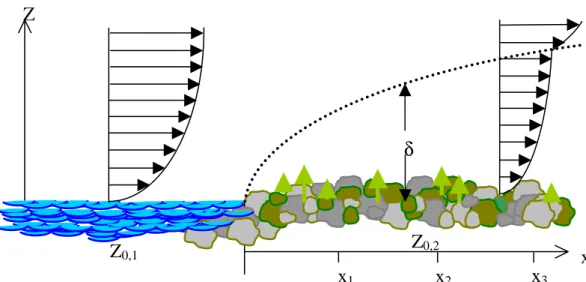
The development of an internal boundary layer at a surface roughness boundary has been widely studied in the past (Stull, 1998 and references therein). At the transition from an ocean surface to land, the advecting air experiences increased drag as a result

5

of increasing surface roughness. However, the surface layer takes some time to fully respond to the change in surface conditions. The air next to the surface experiences an instantaneous reduction in mean speed but the air aloft will not respond immediately. Rather the reduction in wind speed with height propagates vertically at a rate governed by its response to the drag it experiences from the immediately underlying air. Wave

10

breaking on the shoreline will produce large sea salt particles (Kunz, 2002) and this production is likely to be significantly influenced by the developing internal boundary layer and will be retained within it. The inter-tidal zone at Mace Head has previously been shown to be a source of iodocarbons (Carpenter,2003) and these species have been linked with ultrafine particle formation (O’Dowd et al., 2002; McFiggans et al.,

15

1998). The developing internal boundary layer will act to restrict the vertical diffusion of such emissions. It was therefore important to understand the micrometeorology of the internal boundary layer in a range of stability conditions, wind directions and tidal heights during NAMBLEX to establish whether the sample inlets were likely to be within the internal boundary layer and therefore whether they may be impacted by any gas or

20

particle sources in the inter-tidal zone.

Turbulence statistics were calculated from the sonic data every 15 min throughout the experiment Fig. 12. The stress is measured by the covariance of the horizontal and vertical winds and is a measure of the in-situ momentum flux at any given height. Figure12a shows the normalised average stress as a function of height above sea level

25

in three different on-shore wind sectors. There is clearly no perturbation to the stress profile in either the southerly or south-westerly wind sectors at the 15 m level or above

ACPD

Full Screen / Esc

Print Version

Interactive Discussion

EGU but the 10 m level shows an increase in stress, indicating that the internal boundary

layer development has reached between 10 and 15 m at the sampling location. In the north-westerly sector there is some indication that the stress at 15 m has been perturbed, though the effect is considerably smaller than at the levels below. This enhancement may be due to a much steeper coastal bluff in that direction but may also

5

be caused by some interference from the main laboratory, which was 8 m high and was located immediately upwind of the tower in this wind direction. These data show the internal boundary layer height is at or below 15 m in all of the sampled marine air masses during the experiment. Figure 12b shows the impact of tidal height on the shape of the stress profile. There is some indication that the stress perturbation is

10

larger at low tide due to the greater exposure of the inter-tidal coast, however, there is no indication that the perturbation affects the wind profile at 24 m, demonstrating that in all wind directions and tidal conditions the measurements made from the 24 m are free from the immediate influence of the shore. It is likely that measurements made at, or below 10–12 m, will be significantly impacted by shoreline or inter-tidal emissions.

15

Previous work (Carpenter, 2003) has provided evidence for iodocarbon profiles that support these findings. It is recommended that the discontinuities in the surface profile arising from changes in surface roughness be considered when interpreting data at Mace Head that is likely to have significant coastal sources.

7. Conclusions

20

This paper has presented a meteorological overview of the NAMBLEX field campaign, for use in interpreting the chemical measurements. The comparative investigations found that on the whole the ECMWF model analysis at 10 m and 1100 m agreed well with the meteorological measurements, but on a number of days the local winds were very different to the synoptic flow. The greatest discrepancies were observed between

25

1 and 6 August when the winds were light and sea breeze effects dominated. Sea breezes were also observed between 17 and 22 August and on the 25th. On days

ACPD

Full Screen / Esc

Print Version

Interactive Discussion

EGU when the local flow was different from the synoptic, trajectory calculations based on the

ECMWF model should be treated with caution. The UHF radar reflectivity profile have also been used to identify days when the boundary layer could be considered convec-tively mixed up to ∼1 km. In fact such days were rare: when on-shore winds prevailed the boundary layer showed little evidence of active mixing above ∼700 m. Turbulence

5

statistics have been used to assess the development of the internal boundary produced by the change in roughness at the shoreline at the measurements location.

Stress profiles show that in all marine sectors sampled the stress profile is perturbed, indicating the influence of the internal boundary layer, at the 10 m sample level and below. There is some evidence that this may reach 15 m in the north westerly sector,

10

though the terrain and the laboratory may induce artifacts under these conditions. The increased inter-tidal fetch at low tide is measurable in the stress profile but does not show that the internal boundary layer propagates to 24 m, even at low tide. However, sampling at, or below, 15 m may be affected under low tide conditions.

Acknowledgements. The authors would like to thank D. Heard and all their colleagues involved

15

in NAMBLEX. Credit is also due to P. Currier and colleagues at Degreane for their help with the wind profiler. This work was supported by University Facility for Atmospheric Measurements (UFAM), Natural Environmental Research Council (NERC) and British Atmospheric Data Cen-tre (BADC).

References

20

Carpenter, L. J., Liss, P. S., and Penkett, S. A.: Marine organohalogens in the atmosphere over the Atlantic and Southern Oceans, J. Geophys. Res., 108(D9), art. no. 4256, 2003. 3204,

3205

Doviak, R. J. and Zrnic, D. S., Doppler Radar and Weather Observations, Academic Press, 1993. 3194

25

Kunz, G. J., de Leeuw, G., Becker, E., and O’Dowd, C. D.: Lidar observations of atmospheric boundary layer structure and sea spray aerosol plumes generation and transport at Mace

ACPD

Full Screen / Esc

Print Version

Interactive Discussion

EGU Head, Ireland (PARFORCE experiment), J. Geophys. Res., 107(D19), art. no. 8106, 2002.

3204

McFiggans, G., Coe, H., Burgess, R., Allan, J., Cubison, M., Alfarra, M. R., Saunders, R., Saiz-Lopez, A., Plane, J. M. C., Wevill, D. J., Carpenter, L. J., Rickard, A. R., and Monks, P. S.: Direct evidence for coastal iodine particles from Laminaria macroalgae – linkage to

5

emissions of molecular iodine, Atmos. Chem. Phys., 4, 701–713, 2004,

SRef-ID: 1680-7324/acp/2004-4-701.

O’Dowd, C. D., Jimenez, J. L., Bahreini, R., Flagan, R. C., Seinfeld, J. H., Hameri, K., Pirjola, L., Kulmala, M., Jennings, S. G., and Hoffmann, T.: Marine aerosol formation from biogenic iodine emissions, Nature, 417 (6889), 632–636, 2002.

10

Stull, R. B.: An introduction to boundary layer meteorology, Kluwer Academic Publishers, Lon-don, 1988. 3202

ACPD

Full Screen / Esc

Print Version

Interactive Discussion

EGU

Table 1. Characteristics of the UFAM mobile 1290 MHz wind profiler.

Parameter Value Transmitter Frequency 1290 MHz Transmitter Wavelength 23.2 cms−1 Transmitter Bandwidth 10 MHz Beam Width 8.5◦ Peak Power 3500 W Aperture 4 m2 Antenna Gain 25 dB Average Power ‘low mode’ 40 W ‘high mode’ 100 W Duty Cycle ‘low mode’ 1% ‘high mode’ 2.5% Spatial Resolution 500 ns pulse 75 m 1000 ns pulse 150 m 1500 ns pulse 375 m Intrinsic Accuracy Speed <1 ms−1 Direction <10◦

ACPD

Full Screen / Esc

Print Version

Interactive Discussion

EGU

Table 2. Scintec MFas64 technical specifications.

Number of Elements 64 Frequency Range 1650–2750 Hz Beam Angles 0◦, ±22, ±29 Number of frequencies Up to 80, (10 within

a single sequence) Number of vertical layers 100 Thickness of layer 10–250 m Maximum range 1000 m Minimum measurement height 20 m Intrinsic Accuracy

Horizontal speed 0.1–0.3 ms−1 Vertical speed 0.03–0.1 ms−1

Direction 2–3◦

ACPD

Full Screen / Esc

Print Version

Interactive Discussion

EGU

Table 3. Pulse sequence used during NAMBLEX.

Frequency (Hz) Pulse length (m) 2022.0 210 2124.8 150 2227.6 100 2330.4 80 2433.2 50 2536.1 40 2638.9 30 2741.7 20 1919.2 10 1713.6 10

ACPD

Full Screen / Esc

Print Version

Interactive Discussion

EGU

Table 4. Comparison Statistics of the ECMWF model analysis with the wind profiler at 1100 m

(1–15 and 21–31 August) and with the sonic anemometer at 10 m (6–19, 22–24 and 26–31 August).

Altitude 1000 m Parameter speed u v Correlation Coefficient 0.9228 0.9680 0.9302

RMS (ms−1) 1.8148 1.5176 2.1470 Slope 1.0272 0.9680 1.0176 Error in Slope (1σ) 0.0228 0.0268 0.0438

Altitude 10 m

Parameter speed u v Correlation Coefficient 0.8585 0.8937 0.9424

RMS (ms−1) 1.5210 1.3822 1.4558 Slope 1.0607 0.9506 0.9042 Error in Slope (1σ) 0.0411 0.0736 0.0495

ACPD

Full Screen / Esc

Print Version

Interactive Discussion

EGU

Fig. 1. Comparisons for period one between the ECMWF model analysis every 6 h at 10 m

(pink line) and 1000 m (blue line) with measurements by sonic anemometers at 7 m (yellow line), 10 m (red line), 15 m (black line) and 24 m (green line), standard surface anemometer (black dashed line) and UHF wind profiler data (blue triangles) for(a) wind direction and (b)

wind speed. The bold black line on the time axis indicates hours of darkness. On this plot for period one the lower and upper levels have been offset from one another for clarity. Note the close agreement in wind directions measured by the different anemometer make it is often difficult to distinguish between them.

ACPD

Full Screen / Esc

Print Version

Interactive Discussion

EGU

ACPD

Full Screen / Esc

Print Version

Interactive Discussion

EGU

ACPD

Full Screen / Esc

Print Version

Interactive Discussion

EGU

ACPD

Full Screen / Esc

Print Version

Interactive Discussion

EGU

ACPD

Full Screen / Esc

Print Version

Interactive Discussion

EGU

Fig. 6. Comparison of wind profiler and ECMWF zonal velocity of wind at 1000 m during

ACPD

Full Screen / Esc

Print Version

Interactive Discussion

EGU

Fig. 7. 1290 MHz wind profiler data for 4 August 2002 (a) Wind speed and direction (b)

ACPD

Full Screen / Esc

Print Version

Interactive Discussion

EGU

Fig. 8. The same as Fig.7 but for 9 August 2002. Note the clockwise turning of the wind direction with height within the turbulent boundary layer is extremely clear in this picture.

ACPD

Full Screen / Esc

Print Version

Interactive Discussion

EGU

ACPD

Full Screen / Esc

Print Version

Interactive Discussion

EGU

ACPD

Full Screen / Esc

Print Version Interactive Discussion EGU

Z

x

x

x

x

δ

Z

Z

Fig. 11. Schematic of the development of an internal boundary layer arising from a change in

ACPD

Full Screen / Esc

Print Version Interactive Discussion EGU u'w'_(z)/u'w'₍₂₄₎ 0 1 2 3 z / m 0 5 10 15 20 25 30 low tide high tide u'w'_(z)/u'w'₍₂₄₎ 0 1 2 3 z / m 0 5 10 15 20 25 30 SW W NW

Fig. 12. Normalised stress profile, averaged over the entire experimental period as a function