deltaRpkm
An R package for a rapid detection of differential gene presence
between related genomes
Hatice Akarsu
1,2, Lisandra Aguilar-Bultet
3, Laurent Falquet
1,21Department of Biology, University of Fribourg, Switzerland, 2Swiss Institute of Bioinformatics, BUGFri group, Fribourg, Switzerland
3Institute of Veterinary Bacteriology, University of Bern, Switzerland,
Nov 2019
deltaRpkm is an R package whose main purpose is to quickly identify genes potentially involved in a trait of interest by performing a differential analysis of genes coverage between two sets of closely related bacterial genomes. The package provides functions to compute the RPKM, the δRP KM , candidate genes filtering and heatmap plot. It also includes methods to perform some batch effect controls and diagnostic plots.
Contents
1 Prerequisites 3
1.1 Input files . . . 3
1.2 Minimum of R knowledge . . . 3
1.3 R dependencies . . . 4
1.4 Download and install deltaRpkm . . . 4
2 Overview of the pipeline 5 3 Building and loading the coverage table 5 4 Loading the metadata table 6 5 Convert read counts to RPKM values 8 5.1 RPKM formula . . . 8
5.2 Run deltaRpkm::rpkm . . . 8
6 δRP KM values 9 6.1 δRP KM formula . . . 9
6.2 Run deltaRpkm::deltarpkm . . . 9
7 Differential gene presence 9 7.1 Strategy . . . 9
7.2 Run deltaRpkm::deltaRPKMStats . . . 10
7.3 Visual check of the mj distribution . . . 11
7.4 Selected gene set . . . 11
8 Heatmap 12 8.1 Rational . . . 12
8.2 Preparing the RPKM values for the heatmap . . . 12
8.3 Plot heatmap . . . 13
8.4 Tuning heatmap parameters: color breaks . . . 14
9 deltaRpkm performance: downsampling 16 9.1 Dataset size effect on thresholding and gene set selection . . . 16
9.2 Dataset size effect on runtime . . . 18
9.3 Dataset size effect on memory usage . . . 19
9.4 Random datasets . . . 19
10 Binaries and OS platforms 20 10.1 Ubuntu Trusty Tahr (14.04.5 LTS) . . . 20
10.2 Ubuntu Bionic Beaver (18.04.2 LTS) . . . 20
10.3 MacOS High Sierra (10.13.6) . . . 21
1
Prerequisites
1.1
Input files
The deltaRpkm package requires 2 user input files:
1. ametadata table that provides parameter information for inter-group comparisons, with the following mandatory fields:
<sample> <phenotype_1> <phenotype_2> <genome_length> <mapped_reads> <...>
• <sample> the column containing the sample names
• <phenotype_1> the column containing the name of the trait being investigated for the gene differential presence analysis
• <phenotype_2> the column containing the 2nd trait that can be added in the heatmap for comparison
• <genome_length> the column containing the reference genome length
• <mapped_reads> the column containing the total number of mapped reads in each sample
• <...>
These are the minimum required elements to be given to the pipeline; more factors can be included for alternative analyses if desired.
2. acoverage tablethat combines the mapped read counts per gene and per sample, as this: <chr> <start> <end> <geneID> <sample1_readCounts> <sample2_readCounts> <...>
• <chr> the column containing the name of reference genome • <start> the column containing the gene start coordinate • <end> the column containing the gene end coordinate • <geneID> the column containing the gene identifier
• <sample1> the column named by the sample 1 and containing its mapped read counts
• <sample2> the column named by the sample 2 and containing its mapped read counts
• <...>
Please make sure that the input tables follow as much as possible those formats (column order and names for the minimum required information). For instance, the sample names in the
<sample> column of the metadata table MUST be the same as <sample_readCounts> in the
coverage table.
The working examples provided by the package correspond to datasets of different sizes from Listeria monocytogenes (Aguilar-Bultet et al., 2018).
1.2
Minimum of R knowledge
Although deltaRpkm is very simple/user-friendly and comes with an extensive documenta-tion (https://github.com/frihaka/deltaRpkm/tree/master/doc), it assumes a minimum
familiarity with R, e.g installing libraries from CRAN and Bioconductor, awareness of working environment, basic R commands and objects etc.
1.3
R dependencies
The R package deltaRpkm, like any R package, is built upon common R CRAN libraries that should be already installed in your system if you are an R user (ggplot2, ggfortify, dplyr, data.table...).
It also requires some Bioconductor R packages. If not already in your system, please make sure that the following R packages from Bioconductor - sva and Biostrings - are installed:
# f o r R >= 3 . 5 > i f ( ! r e q u i r e N a m e s p a c e ( " B i o c M a n a g e r " , q u i e t l y = TRUE) ) i n s t a l l . packages ( " B i o c M a n a g e r " ) B i o c M a n a g e r : : i n s t a l l ( " s v a " , v e r s i o n = " 3 . 8 " ) B i o c M a n a g e r : : i n s t a l l ( " B i o s t r i n g s " , v e r s i o n = " 3 . 8 " ) # f o r R <= 3 . 4 s o u r c e( " h t t p s : // b i o c o n d u c t o r . o r g / b i o c L i t e . R" ) b i o c L i t e ( " s v a " ) b i o c L i t e ( " B i o s t r i n g s " )
1.4
Download and install deltaRpkm
From GitHub https://github.com/frihaka/deltaRpkm/, download the compressed binary file on a local directory.
If you are familiar with R and have already most of the common R packages (ggplot2, ggfortify, dplyr...), you can install from the terminal with the R CMD INSTALL command:
R CMD INSTALL deltaRpkm_0.1.0_R_x86_64-pc-linux-gnu.tar.gz
and then just install the Bioconductor packages as shown above.
If you are not very familiar with R environment, try rather to install deltaRpkm with the function install.packages(), from inside R/RStudio:
> install.packages("path/2/deltaRpkm_0.1.0_R_x86_64-pc-linux-gnu.tar.gz", repos = NULL,
dependencies = TRUE)
This will download your missing CRAN libraries that are required by deltaRpkm. You will still need to install the Bioconductor packages, as shown above.
2
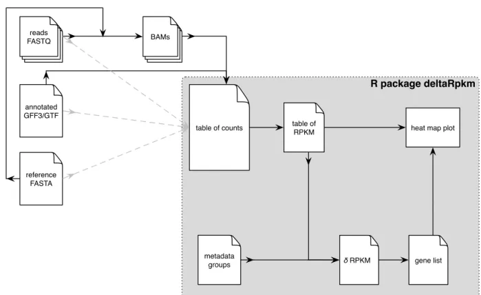
Overview of the pipeline
R package deltaRpkm
metadata groups
table of counts table of RPKM heat map plot
gene list δ RPKM reads FASTQ reference FASTA annotated GFF3/GTF BAMs
Figure 1: Overview of the deltaRpkm pipeline.
3
Building and loading the coverage table
The read counts per gene table must be pre-computed and provided by the user. Below is the command used to build it with bedtools multicov on a terminal:
bedtools multicov -bams aln.1.bam ... aln.n.bam -bed <bed/gff/vcf> > coverage_table.csv
Notes on bedtools multicov:
• any number of bam files can be run together in a batch mode, thus allowing all the samples of the dataset to be included in the coverage table
• do not forget to redirect/output the results into a coverage table
The user can build the read count table with other methods, like the RNA-seq aligner called STAR that maps and produces the coverage table at once.
Please do not forget to ensure that your custom coverage table (either produced by bedtools multicov or by STAR etc) follows the following required format:
• <chr> • <start> • <end> • <geneID> • <sample1_readCounts> • <sample2_readCounts> • <...>
Alternatively, example datasets derived from Aguilar-Bultet et al., 2018 are available in the deltaRpkm package:
> data ( " c o v e r a g e_t a b l e_N51" ) # t h i s c r e a t e s c o v e r a g e_t a b l e d f i n t h e e n v i r o n m e n t
> head ( c o v e r a g e_t a b l e_N51 [ , 1 : 8 ] )
c h r s t a r t end g e n e I D JF4931 JF5172 JF5761 JF5827 1 JF5203_chromosome 318 1674 LMJF5203_00001 3109 1466 5582 5761 2 JF5203_chromosome 1867 3013 LMJF5203_00002 2778 1099 4737 4882 3 JF5203_chromosome 3120 4464 LMJF5203_00003 3218 1473 4914 5365 4 JF5203_chromosome 4577 4865 LMJF5203_00004 947 358 1568 1546 5 JF5203_chromosome 4868 5981 LMJF5203_00005 2578 932 4415 4572 6 JF5203_chromosome 6029 7970 LMJF5203_00006 4125 1853 7018 7681
4
Loading the metadata table
The user must provide a metadata table with some minimum informations/columns about the samples:
• a column containing the trait or characteristic 1 data, that will be used for the RPKM comparisons. This is the main characteristic of interest being studied, i.e the trait of group 1 with the reference genome. This trait is the criteria of categorizing the datasets into 2 distinct groups and the basis of the whole comparison. For example: ”lineage_type” which can include different values but only 2 will be compared. That is why we advise to categorize samples into groups; in the example: Lineage_I and Lineage_II
• a column containing the trait 2 data, that will be used as a colored sidebar of the heatmap: this corresponds to a 2nd characteristic that the user can add to check whether the clustering in the heatmap correlates with this 2nd trait. For example: ”infection_origin”
• reference genome length • total number of mapped reads
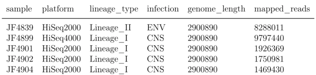
The metadata/design table must be a data frame that looks like this:
Table 1: Example of input metadata table.
sample platform lineage_type infection genome_length mapped_reads JF4839 HiSeq2000 Lineage_II ENV 2900890 8288011
JF4899 HiSeq4000 Lineage_I CNS 2900890 9797440
JF4901 HiSeq2000 Lineage_I CNS 2900890 1926369
JF4902 HiSeq2000 Lineage_I CNS 2900890 1750981
JF4904 HiSeq2000 Lineage_I CNS 2900890 1469430
A working example metadata dataset from deltaRpkm package is shown below:
> data ( " m e t a d a t a_t a b l e_N51" ) # t h i s c r e a t e s m e t a d a t a_t a b l e d f i n t h e e n v
> head ( m e t a d a t a_t a b l e_N51 )
sample p l a t f o r m l i n e a g e_t y p e i n f e c t i o n genome_l e n g t h mapped_r e a d s 1 JF4906 H i S e q 2 0 0 0 L i n e a g e_I CNS 2900890 2042865 2 JF4929 H i S e q 4 0 0 0 L i n e a g e_I CNS 2900890 9469100 3 JF4931 H i S e q 3 0 0 0 L i n e a g e_I I CNS 2900890 5285534
Format the metadata information with deltaRpkm::loadMetadata function, giving in as arguments:
• user_metadata = <data frame of user input design table>
• delta_phenotype_colname = <phenotype 1 column name used to build the 2 cate-gories and perform the comparison>
• heatmapbar_phenotype_colname = <phenotype 2 column name used to build the extra bar in the heatmap>
• samples_colname = <column name containing the sample IDs>
• genome_length_colname = <genomic length (in bp) of the reference genome used for mapping>
• mapped_reads_colname = <total number of mapped reads, for each sample ID>
> d e s i g n_t a b l e <− l o a d M e t a d a t a ( u s e r_m e t a d a t a = m e t a d a t a_t a b l e_N51 , d e l t a_p h e n o t y p e_c o l n a m e = " l i n e a g e_t y p e
" ,
h e a t m a p b a r_p h e n o t y p e_c o l n a m e = " i n f e c t i o n " ,
genome_l e n g t h_c o l n a m e = " genome_l e n g t h " ,
mapped_r e a d s_c o l n a m e = " mapped_r e a d s " )
> head ( d e s i g n_t a b l e )
sample l i n e a g e_t y p e i n f e c t i o n genome_l e n g t h mapped_r e a d s 1 JF4906 L i n e a g e_I CNS 2900890 2042865 2 JF4929 L i n e a g e_I CNS 2900890 9469100 3 JF4931 L i n e a g e_I I CNS 2900890 5285534
5
Convert read counts to RPKM values
5.1
RPKM formula
deltaRpkm uses the Reads Per Kilobase Million RPKM - a standard RNA-seq metrics that normalizes the read counts per gene for Sequencing Depth and Gene Length:
with Ns being the total number of read counts in the sample, scalingF actor = Ns 106 (1) RP M = readCountP erGene scalingF actor (2) RP KM = RP M geneLength.10−3 (3)
The equation (2) corresponds to the normalization of the read counts by the sample sequencing depth; and equation (3) corresponds to the normalization by the gene length.
5.2
Run deltaRpkm::rpkm
Run the following deltaRpkm::rpkm function to compute the RPKM values of each gene, in each sample:
> r p k m t a b l e <− rpkm ( u s e r_m e t a d a t a = d e s i g n_t a b l e ,
c o v e r a g e_t a b l e = c o v e r a g e_t a b l e_N51 , d e l t a_p h e n o t y p e_c o l n a m e = " l i n e a g e_t y p e " , h e a t m a p b a r_p h e n o t y p e_c o l n a m e = " i n f e c t i o n " ) > head ( r p k m t a b l e ) sample g e n e I D l i n e a g e_t y p e i n f e c t i o n r e a d s rpkm 1 JF4906 LMJF5203_00001 L i n e a g e_I CNS 1177 425 2 JF4906 LMJF5203_00002 L i n e a g e_I CNS 952 406 3 JF4906 LMJF5203_00003 L i n e a g e_I CNS 1080 393
6
δRP KM values
6.1
δRP KM formula
The analysis is centered around a pairwise comparison of gene presence/absence between genomes categorized into two different groups following the selected trait or feature:
• a group 1 that shares the trait A of the reference genome • a group 2 that does not have the reference trait A
For each pairwise comparison of a gene j between a genome x from group 1 and a genome y from group 2, deltaRpkm::deltarpkm function computes the difference of their RPKM values at gene j (δRP KMjxy) as:
δRP KMjxy = RP KMjx− RP KMjy (4)
6.2
Run deltaRpkm::deltarpkm
> d e l t a r p k m_t a b l e <− d e l t a r p k m ( rpkm_t a b l e = r p k m t a b l e ,
g e n e s_names = unique ( r p k m t a b l e $ g e n e I D ) , s a m p l e s_c o l n a m e = " s a m p l e " ,
d e l t a_p h e n o t y p e_c o l n a m e = " l i n e a g e_t y p e " , r e f e r e n c e_sample = " JF5203 " , n o n r e f_d e l t a_p h e n o t y p e = " L i n e a g e_I I " ) > head ( d e l t a r p k m_t a b l e ) g e n e I D sample . g r o u p 1 l i n e a g e_t y p e . g r o u p 1 i n f e c t i o n . g r o u p 1 r e a d s . g r o u p 1 rpkm . g r o u p 1 sample . g r o u p 2 l i n e a g e_t y p e . g r o u p 2 i n f e c t i o n . g r o u p 2 r e a d s . g r o u p 2 rpkm . g r o u p 2 d e l t a r p k m 1 LMJF5203_00001 JF4906 L i n e a g e_I CNS 1177 425 JF4931 L i n e a g e_I I CNS 3109 433 −8 2 LMJF5203_00001 JF4906 L i n e a g e_I CNS 1177 425 JF5172 L i n e a g e_I I CNS 1466 520 −95 3 LMJF5203_00001 JF4906 L i n e a g e_I CNS 1177 425 JF5761 L i n e a g e_I I ENV 5582 465 −40
This run might take a few minutes, depending on the size of the datasets.
7
Differential gene presence
7.1
Strategy
The deltaRpkm package main feature is to screen for the preferential presence of genes in the reference genome group, versus a comparison group.
We use the method deltaRpkm::deltaRPKMStats to infer this set of genes, since they could potentially be involved in the reference genome group trait (<lineage_type> =”Lin-eage_type_I”). This function:
1. computes for each gene j the median value of all its δRP KM (mj) derived from the sample pairwise comparisons. Note: a negative median value of all δRP KM of a given gene would mean that this gene is ”preferentially present” in the comparison samples of group 2 than in the reference genome group 1
2. calculates the standard deviation s of all the mj values in the analysis
3. selects genes as present in the reference genome group 1 based on an arbitrary threshold of 2.s:
selectedGene : mj >= 2.s (5)
In other words, a gene j having a median δRP KM value greater than 2.s will be consid-ered as ”preferentially present” in the reference genome group 1 (with <lineage_type>
=”Lineage_type_I”) than in the comparison group 2 (with <lineage_type> =”Lineage_type_II”).
7.2
Run deltaRpkm::deltaRPKMStats
> s t a t s_t a b l e <− deltaRPKMStats ( d e l t a r p k m_t a b l e = d e l t a r p k m_t a b l e ) > head ( s t a t s_t a b l e ) g e n e I D sample . g r o u p 1 l i n e a g e_t y p e . g r o u p 1 i n f e c t i o n . g r o u p 1 r e a d s . g r o u p 1 rpkm . g r o u p 1 sample . g r o u p 2 l i n e a g e_t y p e . g r o u p 2 1 LMJF5203_00001 JF4906 L i n e a g e_I CNS 1177 425 JF4931 L i n e a g e_I I 2 LMJF5203_00001 JF4906 L i n e a g e_I CNS 1177 425 JF5172 L i n e a g e_I I 3 LMJF5203_00001 JF4906 L i n e a g e_I CNS 1177 425 JF5761 L i n e a g e_I I i n f e c t i o n . g r o u p 2 r e a d s . g r o u p 2 rpkm . g r o u p 2 d e l t a r p k m d e l t a r p k m_median d e l t a r p k m_medianSD t h r e s_SD_median_v a l u e s e l e c t e d_g e n e 1 CNS 3109 433 −8 −31 1 1 4 . 2 4 2 2 8 . 4 8 − 2 CNS 1466 520 −95 −31 1 1 4 . 2 4 2 2 8 . 4 8 − 3 ENV 5582 465 −40 −31 1 1 4 . 2 4 2 2 8 . 4 8 −The default threshold value to select genes is based on 2.s. But this threshold can be changed in the deltaRpkm::deltaRPKMStats parameter min_SD_foldChange, e.g:
> s t a t s_t a b l e_f c n e w <− deltaRPKMStats ( min_SD_f o l d C h a n g e = 1 . 5 , d e l t a r p k m_t a b l e = d e l t a r p k m_t a b l e )
Note that the column selected_gene contains information about whether a given gene should be selected as present preferentially in the reference genome group (noted as "+") or not (noted as "-"). This column will be used later to filter the relevant genes.
7.3
Visual check of the m
jdistribution
With the function deltaRpkm::median_plot it is possible to check visually the median δRP KM value of every gene (one dot per gene).
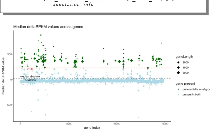
> median_p l o t ( data_t a b l e = s t a t s_t a b l e ,
g e n e_a n n o t a t i o n_t a b l e = c o v e r a g e_t a b l e_N51 ) # g e n e s a n n o t a t i o n i n f o
Figure 2: Median δRP KM values for all genes. Plot output from deltaRpkm::median_plot.The negative median δRP KM values correspond to genes that appear as better covered in the comparison group 2 than in the reference genome group 1. Note: the gene index value reflects the genomic coordinates since they are ordered as the gene names (these later being themselves given during de novo annotation based on the genomic coordinates, roughly speaking).
The genes in dark green in Figure 2 correspond to the set of genes present in the reference genome group 1 and potentially linked to the trait of interest ("lineage_type").
7.4
Selected gene set
For a given threshold value of median δRP KM (by default 2.s of all median δRP KM values), we can simply extract the genes appearing as differentially present in the reference genome group 1 (green dots in the Figure 2):
> d i f f e r e n t i a l_p r e s e n t_g e n e s <− unique ( s t a t s_t a b l e [ s t a t s_t a b l e $ s e l e c t e d_g e n e %i n% "+" , ] $ g e n e I D ) > l e n g t h ( d i f f e r e n t i a l_p r e s e n t_g e n e s ) > [ 1 ] 173 > head ( d i f f e r e n t i a l_p r e s e n t_g e n e s ) > [ 1 ] "LMJF5203_00013 " "LMJF5203_00014 " "LMJF5203_00015 " "LMJF5203_
00033 " "LMJF5203_00034 " "LMJF5203_00035 "
This gene set can be used to perform various functional clustering analysis. We propose in the package a method to build a summary heatmap of their RPKM values and how they relate (or not) to a second trait of interest.
8
Heatmap
8.1
Rational
The idea is to analyse how the RPKM values of the genes specific to the reference genome group 1 distribute across all samples of group 1 and group 2. The aim is:
• to confirm (or infirm) that the heatmap clustering of the samples into two distinct cate-gories is coherent with the initial group 1 and group 2 definition. Typically, the selected genes should present in overall higher RPKM values in the reference genome group 1 than in group 2. But it is not always the case.
• to investigate at a higher resolution the homogeneity of each group
Thus deltaRpkm allows to investigate the clustering of the selected genes based on their RPKM values computed earlier. A putative correlation with the second trait can be visualized by adding a color bar corresponding to this second trait given in the metadata table - which is "infection" in the working example dataset.
The heatmap plot is made with the deltaRpkm::rpkmHeatmap function, derived from the gplots::heatmap.2 method (Warnes et al., 2018).
8.2
Preparing the RPKM values for the heatmap
The heatmap will focus only on the RPKM values of the set of genes that are relevant, i.e the ones that appear as differentially present in the reference genome group 1 (see the darkgreen dots in Figure 2).
For this, we first subset the RPKM data table and keep only the rows/genes that were selected using the deltaRpkm::subsetRPKMTable:
# S u b s e t t h e RPKM t a b l e f o r t h e s e l e c t e d g e n e s
> heatmap_t a b l e <− subsetRPKMTable ( rpkm_t a b l e = r p k m t a b l e , u s e r_m e t a d a t a = d e s i g n_t a b l e ,
d e l t a_p h e n o t y p e_c o l n a m e = " l i n e a g e_t y p e " , h e a t m a p b a r_p h e n o t y p e_c o l n a m e = " i n f e c t i o n " , sd_f i l t e r e d_g e n e s = d i f f e r e n t i a l_p r e s e n t_g e n e s ) > head ( heatmap_t a b l e ) sample l i n e a g e_t y p e i n f e c t i o n LMJF5203_00013 LMJF5203_00014 LMJF5203 _00015 LMJF5203_00033 LMJF5203_00034 LMJF5203_00035 LMJF5203_ 00036 1 JF4906 L i n e a g e_I CNS 607 450 630 421 445 521 553
2 JF4929 L i n e a g e_I CNS 581 397 498 456 447 427 423 3 JF4931 L i n e a g e_I I CNS 0 0 0 68 1 2 1
Then the subsetted RPKM values data frame is converted to a matrix (since this is the required format for the heatmap function) using thedeltaRpkm::convertHeatmapToMatrix func-tion:
# C o n v e r t t h e s u b s e t t e d RPKM t a b l e t o a m a t r i x
> heatmap_matrix <− c o n v e r t H e a t m a p T o M a t r i x ( w i d e_rpkm_t a b l e = heatmap_ t a b l e ,
d e l t a_p h e n o t y p e_c o l n a m e = " l i n e a g e_t y p e " , h e a t m a p b a r_p h e n o t y p e_c o l n a m e = " i n f e c t i o n " ) > head ( heatmap_matrix ) LMJF5203_00013 LMJF5203_00014 LMJF5203_00015 LMJF5203_00033 LMJF5203_00034 LMJF5203_00035 LMJF5203_00036 LMJF5203_00037 LMJF5203_00038 LMJF5203_00082 LMJF5203_00083 LMJF5203_00084 JF4906 607 450 630 421 445 521 553 472 491 619 352 450 JF4929 581 397 498 456 447 427 423 412 484 0 0 0 JF4931 0 0 0 68 1 2 1 0 1 0 18 457
It is important to note that the heatmap matrix must contain sample names as row names.
8.3
Plot heatmap
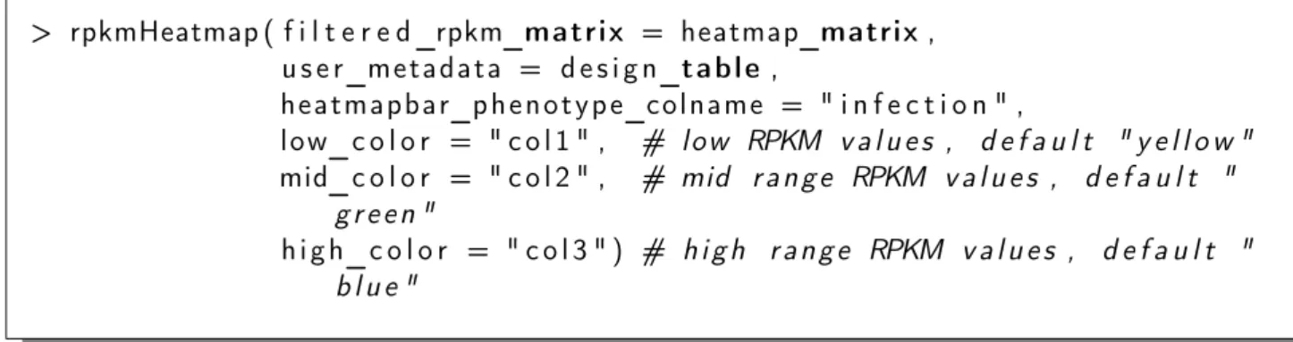
Finally, we create a summary plot as a heatmap to highlight difference in the RPKM values of the selected genes between samples of group 1 and group 2, using thedeltaRpkm::rpkmHeatmap function:
> rpkmHeatmap ( f i l t e r e d_rpkm_matrix = heatmap_matrix , u s e r_m e t a d a t a = d e s i g n_t a b l e ,
h e a t m a p b a r_p h e n o t y p e_c o l n a m e = " i n f e c t i o n " )
This creates an output heatmap file deltaRpkm_heatmap.tiff in the working directory. The heatmap for the example dataset (Listeria monocytogenes, N=51 ) is shown in Figure 3. It confirms the clustering of the samples into the initial two categories: group 1 samples cluster together on the upper part corresponding to high RPKM values, while group 2 samples cluster together in the lower part of the heatmap with lower RPKM values, for the selected gene set. The heatmap colors can be easily changed with the color break parameters:
> rpkmHeatmap ( f i l t e r e d_rpkm_matrix = heatmap_matrix , u s e r_m e t a d a t a = d e s i g n_t a b l e , h e a t m a p b a r_p h e n o t y p e_c o l n a m e = " i n f e c t i o n " , l o w_c o l o r = " c o l 1 " , # l o w RPKM v a l u e s , d e f a u l t " y e l l o w " mid_c o l o r = " c o l 2 " , # mid r a n g e RPKM v a l u e s , d e f a u l t " g r e e n " h i g h_c o l o r = " c o l 3 " ) # h i g h r a n g e RPKM v a l u e s , d e f a u l t " b l u e "
See the next section for more on color breaks tuning.
8.4
Tuning heatmap parameters: color breaks
deltaRpkm::rpkmHeatmap comes with various parameters options (see ?rpkmHeatmap), some derived from the original gplots::heatmap.2, and some specific to deltaRpkm anal-ysis.
In particular, the heatmap color breaks can be adjusted with i) the binsize (default 200), ii) the lower_limit (default value 300) and iii) upper_limit (default value 550) arguments. These values are based on the distribution of the RPKM values and correspond to the lower and upper boundary RPKM values of the main peak:
> h i s t ( r p k m t a b l e $rpkm , f r e q = FALSE , b r e a k s = 1 0 0 0 )
Figure 4: Distribution of RPKM values: inferring the heatmap color breaks from the his-togram main peak boundary values. The lower (∼300) and upper (∼550) values of RPKM are used in the deltaRpkm::rpkmHeatmap to adjust the heatmap color breaks. Working dataset Listeria monocytogenes, N=51.
Also, deltaRPKM proposes some methods to infer these RPKM boundary values with the function deltaRpkm::boundaries:
Figure 3: RPKM v alues distribution of the selected across samples from group 1 and group 2. Plot output from deltaRpkm::rpkmHeatmap . The samples cluster follo wing the trait 1 (”lineage_t yp e”), with group 1 annotated as ”Lineage_I” and group 2 annotated as ”Lineage_I I”. Most of the selected genes app ear with a lo w RPKM v alue in group 2 cluster, ev en though some gr oup 2 samples presen t high RPKM v alues (blue pixels) for certain geneIDs, suggesting these genes as p oten tial false p ositiv es.
# d e f a u l t method m c l u s t > r e s <− b o u n d a r i e s ( x = r p k m t a b l e $rpkm ) > r e s $ b o u n d a r i e s_d f b o u n d a r i e s rpkm_v a l u e s 1 lower_l i m i t 300 2 upper_l i m i t 624 > r e s <− b o u n d a r i e s ( x = r p k m t a b l e $rpkm , s t r a t e g y = " r a t i o s " ) > b o u n d a r i e s rpkm_v a l u e s 1 lower_l i m i t 295 2 upper_l i m i t 585 > r e s <− b o u n d a r i e s ( x = r p k m t a b l e $rpkm , s t r a t e g y = " q u a r t i l e s " ) > b o u n d a r i e s rpkm_v a l u e s b o u n d a r i e s rpkm_v a l u e s 1 lower_l i m i t 383 2 upper_l i m i t 487
deltaRpkm::boundariesapplies by default the mclust parameter, which is derived from the method mclust::densityMclust. This can be changed with the parameter strategy. The boundary RPKM values can be simply extracted as res$boundaries_df containing the RPKM boundary values of interest.
Feel free to play with these RPKM boundary and color break parameter values in rpkmHeatmap function and observe the effect(s) on the heatmap readout.
9
deltaRpkm performance: downsampling
The initial Listeria monocytogenes dataset of N=225 samples is downsampled up to N=7 sam-ples. Each dataset is run through deltaRpkm pipeline and the different outcomes are compared.
9.1
Dataset size effect on thresholding and gene set selection
The gene differential presence is based on a threshold value defined as 2 times (default value) the standard deviation of the medians of δRP KM values. The median plots (Figure 2) for all the datasets of different sizes can be summarized in a single boxplot per gene, as shown in Figure 5.
2*SD (N51) −1000 −500 0 500 0 1000 2000 3000 gene index median δ RPKM datasets sizes N=51 N=225 Boxplots of median δ RPKM values across N=24 dataset sizes, per gene
Figure 5: Dataset size effect on the median δRP KM distribution (boxplots series). 24 datasets of different sizes (N=225 to N=7 samples) are plotted as boxplots, one per gene. Datasets with N=51 and N=225 samples are highlighted to evaluate the degree of δRP KM variation between datasets of different sizes.
The boxplot series of Figure 5 shows that most of the selected genes present a stable median δRP KM distribution across all dataset sizes (bars fully above the 2.s threshold).
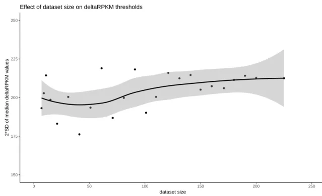
● ● ● ● ● ● ● ● ● ● ● ● ● ● ● ● ● ● ● ● ● ● ● ● 150 175 200 225 250 0 50 100 150 200 250 dataset size 2*SD of median deltaRPKM v alues
Effect of dataset size on deltaRPKM thresholds
Figure 6: Dataset size effect on the 2*SD(median δRP KM ) thresholding values. The smooth line is built with loess() method; confidence interval in grey.
● ● ● ● ● ● ● ● ● ● ● ● ● ● ● ● ● ● ● ● ● ● ● ●
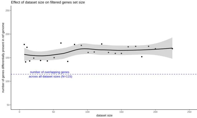
number of overlapping genes across all dataset sizes (N=115)
50 100 150 200 250 0 50 100 150 200 250 dataset size n
umber of genes diff
erentially present in ref genome
Effect of dataset size on filtered genes set size
Figure 7: Dataset size effect on genes differentially present in reference genome. The smooth line is built with loess() method; confidence interval in grey.
9.2
Dataset size effect on runtime
The runtime increases linearly with the dataset size (Figure 8), but it remains reasonably low.
● ● ●● ● ● ● ● ● ● ● ● ● ● ● ● ● ● ● ● ● ● ● ● y=0.08x−2.2 (R^2=0.93) 0 10 20 30 0 50 100 150 200 250 dataset size runtime (min)
Effect of dataset size on deltaRpkm runtime in R
Figure 8: Dataset size and runtime when using deltaRpkm. Including the pipeline steps of RPKM computing, batch effect correction, computing δRP KM values, statistics, gene selection and plotting heatmap. Analysing with deltaRpkm a large dataset of N=225 samples takes < 20min in total in R 3.4.4 (under Ubuntu 14.04.5 LTS).
9.3
Dataset size effect on memory usage
The memory requirement by deltaRpkm analysis grows with the sample size, but in a rather linear way: expect ∼400M every N∼20 samples. So one should be able to run a dataset of up to N∼800 samples on a normal desktop machine with 16G of RAM.
● ● ●● ● ● ● ● ● ● ● ● ● ● ● ● ● ● ● ● ● ● ● ● y = 0.01x−0.29 (R^2=0.93) 0 2 4 6 8 0 50 100 150 200 250 dataset size memor y usage (G)
Effect of dataset size on memory usage in R
Figure 9: Dataset size and memory usage when using deltaRpkm. The pipeline uses < 4G of memory for a dataset of N=225 samples, when ran in R 3.4.4 (under Ubuntu 14.04.5 LTS).
9.4
Random datasets
Random datasets confirm the robustness of selected genes with the deltaRpkm method (Figure 10). When comparing datasets of different sizes (N=51, N=101, N=225) maintaining the original group classification, most of the genes identified as differentially present in the group 1 are conserved across datasets (Figure 10(a), N=144). While on the other hand, the gene sets derived from random groupings are small and not consistent (Figure 10(b), N=0).
3 1 3 2 144 13 10 N51 N101 N225
(a) real groups
33 0 39 13 0 8 56 N51 N101 N225 (b) random groups
Figure 10: Real versus random group classification: random group assignment gives non-robust gene sets across different sizes of datasets. deltaRpkm Listeria monocytogenes datasets. Batch effect corrected.
10
Binaries and OS platforms
10.1
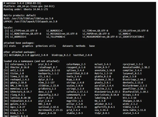
Ubuntu Trusty Tahr (14.04.5 LTS)
The Linux binary has been built and tested withR 3.4underUbuntu 14.04 LTS (Trusty Tahr):
Figure 11: Session info in R 3.4.4, with RStudio 1.0.143, run under Ubuntu 14.04.5 LTS.
10.2
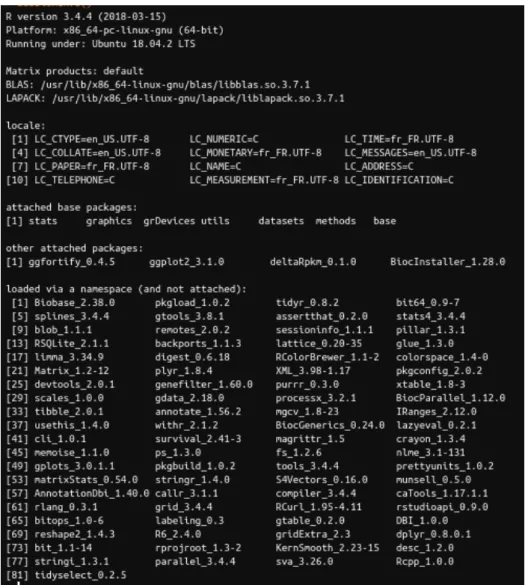
Ubuntu Bionic Beaver (18.04.2 LTS)
The Linux binary has been built and tested with R 3.4 under Ubuntu 18.04.2 LTS (Bionic Beaver):
Figure 12: Session info in R 3.4.4, with RStudio 1.1.463, run under Ubuntu 18.04.2 LTS.
10.3
MacOS High Sierra (10.13.6)
The MacOS binary has been built and tested with R 3.4 under MacOS 10.13.6 (High Sierra):
Figure 13: Session info in R 3.4.0 with RStudio 1.0.143, run under MacOS 10.13.6.
10.4
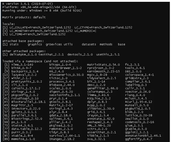
Windows10
The Windows binary has been built and tested with R 3.6 underWindows10: