The CAFE experiment : a joint seismic and MT investigation of the Cascadia subduction system

(1)

The CAFE experiment:

A joint seismic and MT investigation of the Cascadia subduction system

By

R Shane McGary

B.S., Texas A&M University, 2007

Submitted in partial fulfillment of the requirements for the degree of

Doctor of Philosophy

at the

MASSACHUSETTS INSTITUTE OF TECHNOLOGY

and the

A ITUTI

WOODS HOLE OCEANOGRAPHIC INSTITUTION

February, 2013

The author hereby grants to MIT and WHOI permission to reproduce and to distribute publicly paper and electronic copies of this thesis document in whole or in part in any medium now

known or hereafter created.

Signature of Author

Joint Program in Geophysics Massachusetts Institute of Technology And Woods Hole Oceanographic Institution (date of final thesis submission)

Certified by

Rob L. Evans Thesis Supervisor

Accepted by

Rob L. Evans Chair, Joint Committee for Geology & Geophysics Woods Hole Oceanographic Institution

(2)

Abstract

In this thesis we present results from inversion of data using dense arrays of collocated seismic and magnetotelluric stations located in the Cascadia

subduction zone region of central Washington. In the migrated seismic section, we clearly image the top of the slab and oceanic Moho, as well as a velocity increase corresponding to the eclogitization of the hydrated upper crust. A deeper velocity increase is interpreted as the eclogitization of metastable gabbros, assisted by fluids released from the dehydration of upper mantle

chlorite. A low velocity feature interpreted as a fluid/melt phase is present above this transition. The serpentinized wedge and continental Moho are also imaged. The magnetotelluric image further constrains the fluid/melt features, showing a rising conductive feature that forms a column up to a conductor indicative of a magma chamber feeding Mt. Rainier. This feature also explains the disruption of the continental Moho found in the migrated image. Exploration of the

assumption of smoothness implicit in the standard MT inversion provides tools that enable us to generate a more accurate MT model. This final MT model clearly demonstrates the link between slab derived fluids/melting and the Mt. Rainier magma chamber.

(3)

Acknowledgements

Funding for this work was made possible by the American Society for Engineering education through a National Defense Science and Engineering Fellowship, and by the National Science Foundation through two grants for the CAFE and CAFE MT projects.

A

S

I would also like to thank Ken Creager, Geoff Abers, Phil Wannamaker, Virginia Maris, Mike Brown, and Anna Kelbert for their part in the acquisition of data, Fred Pearce and Chin-Wu Chen for their help with the seismic migration codes, Anne Pommier for her help with connecting conductivity to petrology,

and Jimmy Elsenbeck for his assistance with the various MT codes.

I would also like to thank the members of my thesis committee, Dan Lizarralde, Alison Malcolm, Alison Shaw, and Horst Marschall, along with the chair of my thesis defense, Juan Pablo Canales.

Special thanks to my co-advisor, Stephane Rondenay, and my primary advisor Rob Evans, without whom none of this would have been possible.

And finally, special thanks to my wife Carrie and son Ian for their continued support throughout this process.

(4)

1. Introduction

Many of the natural hazards associated with subduction zones are intimately tied to the release of fluids bound within the subducting slab. Intraslab

earthquakes have been linked with a process in which fluids released during the transformation of hydrated metabasalts to eclogite in the upper crust increases pore pressure, thereby reactivating pre-existing faults (Kirby et al., 1996, Hacker et al., 2003b, Preston et al., 2003). Slow slip and low frequency tremor, which have been tentatively linked with the periodicity of great megathrust

earthquakes (Mazzotti and Adams, 2004), can be explained by episodic buildup and release of fluid pore pressure across plate boundaries down-dip of the locked zone (Abers et al., 2009, Audet et al., 2010). Most arc magmas are also generally believed to be generated by flux melting that occurs when dehydration reactions in the oceanic crust and uppermost mantle release fluids into the continental asthenosphere (Ulmer and Trommsdorff, 1995, Kirby et al., 1996).

Finally, density increases associated with dehydration have been linked with changes in slab dip and increased stresses within the slab (Klemd et al., 2011).

(7)

While recent investigations have dramatically improved our understanding of the distribution and cycling of fluids in subduction systems, many questions remain open. Advances in the understanding of the phase transformations that occur within the subducting lithosphere (Poli and Schmidt, 2002, Hacker et al., 2003a and references within, Hacker, 2008) have given us the tools to better interpret geophysical evidence. Improvements in the thermal modeling of subduction zones such as the use of olivine rheology in the mantle wedge (van Keken et al., 2002) and decoupling at the cold nose of the wedge (Wada and Wang, 2009) have aided in the development of a consistent set of thermal models for subduction systems worldwide (Syracuse et al., 2010). Application of the phase transformations along the P-T regimes predicted by the thermal models has made it possible to predict depth dependent fluid flux for the global suite of subduction zones (van Keken et al., 2011).

Cascadia is an attractive setting for studying the fluid distribution and dynamics in subduction zones for a variety of reasons. It has been thoroughly investigated using a variety of geological and geophysical methods over a number of decades, so much is known about both the surface geology and the structure of the subsurface. As the slab is young and hot, it is expected to release a significant fraction of its fluids in the forearc, suggesting that the evidence of fluids should be more pronounced here than they would be in a cooler setting.

(8)

Finally, the connection between these fluid processes and the associated tectonic and volcanic hazards that potentially threaten a number of densely populated areas underline the importance of understanding the subduction fluid cycle in Cascadia.

For all of these reasons, the Cascadia region has been the subject of extensive geophysical work. While much of the geophysical exploration of the region has involved seismology, the magnetotelluric method has also been employed to good effect. Magnetotellurics is attractive because while it is sensitive to a completely different set of rock properties than are seismic methods (Hellfrich, 2003, Jones et al., 2009), velocity and conductivity are often correlated (Stanley et al., 1990, Jones et al., 2009), either directly or simply in the fact that at distinct geological boundaries both parameters are likely to change (Gallardo, 2007, Moorkamp et al., 2007). It is therefore tempting to utilize both types of data in our interpretations, particularly where the data profiles are collocated (Gallardo and Meju, 2007).

While much work in the past has simply been a matter of questioning whether an interpretation of one type of data is consistent with a previous interpretation of a different type, there have been several recent efforts to combine two (or more) types of

data on a more fundamental level. The rationale behind joint inversion of multiple data sets is to improve resolution, diminish the influence of noise, and reduce the inherent non-uniqueness by providing additional constraints (Gallardo, 2007, Moorkamp et al.,

(9)

2007). While the values of velocity and resistivity have been compiled for a wide range of geological and physical conditions (Hacker, 2003a, Jones et al., 2009), there exists no fundamental relationship between the two physical properties (Bedrosian et al., 2007). Still, as we stated above, the two properties do tend to be reasonably well correlated in the subsurface, and several different approaches to joint inversion of seismic and electromagnetic data have been attempted. Some of the techniques utilized to date include stochastic optimization methods such as genetic algorithms (Moorkamp et al., 2007), physical property gradient methods (often combined with structural constraints) such as the cross-gradient (Gallardo, 2007, Hu et al., 2008, Gallardo and Meju, 2007), and statistical correlation methods such as cluster analysis (Bedrosian et al., 2007, Munoz et al., 2010).

None of the joint inversion methods mentioned above address this particular combination of ideas in a completely satisfactory way. They all rely in some way on the natural relationship between the distribution of the resistivity and velocity values. The distribution of resistivity values near sharp boundaries in the MT inversion is smoothed by design (which directly impacts the gradient as well), creating an artificial difference that the joint inversions would attempt to resolve as a natural phenomenon.

A different way to look at the use of multiple data sets is to attempt to use the strengths of one technique to mitigate weaknesses inherent in another. For example, the magnetotelluric technique typically employs a smoothness constraint to control the

(10)

resolution of structure to that required by the data. Of course, sharp boundaries exist in the subsurface, and these are often not well resolved by the method. This suggests that we might attempt to combine MT with a method that is well suited to illuminating sharp boundaries. Teleseismic migration is one particularly appealing candidate, involving backpropagation of a scattered wavefield to the scattering points in the subsurface (Rondenay, 2009), thereby highlighting the very boundaries we hope to resolve.

This is the approach we take in the current study, analyzing data collected at dense arrays of roughly collocated passive seismic and magnetotelluric stations. We analyze the two data sets independently, using Generalized Radon Transform (GRT) migration for the seismic data, and Non-Linear Conjugate Gradient (NLCG) inversion for the magnetotelluric data. We then perform the magnetotelluric inversion again, this time

incorporating the a priori information obtained during the GRT migration into the inversion.

While there are valid reasons for searching for the smoothest resistivity model in the absence of a priori information, the presence of such information, particularly with respect to the location of sharp boundaries, warrants another approach. While

inversion methods allow us to create models that fit the data as closely as desired, there is a tradeoff between resolving structure and generating false structure from noise that tips decidedly in favor of the latter as the misfit becomes small. For any reasonable

(11)

selection of misfit, there are an infinite number of solutions that fit the data equally well (Parker, 1994, Zhdanov, 1993). The selection of a specific model is necessarily a

subjective process involving the incorporation of a priori information and/or assumptions about the nature of the distribution of the measured parameter in the subsurface.

The conventional way to think about such problems is as a minimization of the Tikhonov parametric functional (Tikhonov and Arsenin, 1977),

T(m)=(m)+As(m) ₍₁₎

where m is a matrix representing a distribution of geophysical parameters within some space, O(m) is the misfit functional described by

(2)

where d is the observed data and Fm the data predicted by the model, and s(m) is a functional that represents assumptions or a priori information that the worker has chosen to include, with its relative importance determined by the regularization

parameter A (Tikhonov and Arsenin, 1977, Parker, 1994, Mehanee and Zhdanov, 2002). 0(m)= I I Fm-d 11I2

(12)

Equations (1) and (2) offer at least three fundamental ways in which we might express a preference for one model over another. The first of these is simply to fix the value of the model parameter over some spatial distribution. For example, in coastal magnetotelluric surveys, it is standard practice to include in the model a fixed

distribution of highly conductive cells to represent the ocean, thereby excluding all models that don't include a conductor where we know one to exist.

A second method is to include an additional parameter within the misfit functional, jointly inverting for two nominally independent data sets. The inclusion of a second set

of data can improve resolution and reduce the impact of noise, thereby constraining the range of possible models (Gallardo, 2007). The set of models that explains two (or more) datasets to a given misfit is both smaller and more compelling than the set that explains one but not necessarily the other.

Finally, we can utilize the stabilizing functional s(m) to express preference for a given subset of models. While several stabilizing functions have been successfully used (least squares, minimum norm of the gradient, distance from an a priori model, etc.) in various geophysical applications (Smith et al., 1999, Mehanee and Zhdanov, 2002, de Groot-Hedlin and Constable, 2004), many magnetotelluric algorithms employ the

minimum norm of the Laplacian, which will seek the smoothest model possible that fits the data (for a given misfit). The argument is that by seeking the smoothest model (again, for a sufficiently large misfit), only structure explicitly required by the data will

(13)

be resolved (de Groot-Hedlin and Constable, 1990). In nature, sharp geoelectric

boundaries do of course exist, and smooth algorithms may not sufficiently resolve these boundaries (Smith et al., 1999, de Groot-Hedlin and Constable, 2004, Mehanee and Zhdanov, 2002).

In order to overcome these difficulties, several algorithms have been developed that allow for sharp boundaries by making different global assumptions about the

distribution of the modeled parameter in the subsurface, for example by favoring models made up of layers (Smith et al., 1999, de Groot-Hedlin and Constable, 2004) or containing primarily blocky structure (Mehanee and Zhdanov, 2002). Of course, each of these global algorithms present trade-offs, and are effective largely to the extent that the underlying assumptions are accurate throughout the modeled space. While a priori knowledge regarding the location and nature of sharp discontinuities can be an

extremely useful implement in resolving the associated structure (de Groot-Hedlin and Constable, 1990), its utility in resolving a sufficiently complicated subsurface is

dependent on the extent to which it can be effectively applied locally.

Inversion packages such as WinGlink and Occam allow for the elimination of the penalty for roughness along presumed discontinuities (de Groot-Hedlin and Constable,

1990, Rodi and Mackie, 2001), and while this tool has been used to good effect (Matsuno et al., 2010), it is but a tentative first step in exploring the possibilities for spatially-dependent stabilizing functionals. While de Groot-Hedlin and Constable rightly point

(14)

out that one should use such tools cautiously as "incorrect placement of boundaries may produce misleading results", we must also recognize that their use is simply trading one set of assumptions for another and we should be cautious in any event.

Chapter 2 presents high resolution images from 2-D GRT migration of data

collected from a dense array of 41 broadband seismometers located in a roughly east to west transect across central Washington State. We see a dipping low velocity layer that we interpret to be the descending oceanic crust, underlain by a positive velocity

transition that we take to be the oceanic Moho. A fading velocity contrast suggests the transformation of hydrated basalt in the upper crust to eclogite, but also shows the retention of fluids to depths of 80 km or more. A low velocity feature above the slab is consistent with a fluid/melt phase released at depths of 80-100 km.

Previous GRT work conducted across Vancouver Island/British Columbia to the north and Oregon to the south allow us to make comparisons and investigate regional implications. Earthquake distribution combined with our results suggest that the fluid release at 80 km depth in central Washington is due to the dehydration of chlorite

harzburgite in the uppermost mantle and subsequent transformation of lower crustal metastable gabbros to eclogite. The extent to which this occurs in central Washington appears to be unique for Cascadia.

(15)

Chapter 3 follows up with high resolution images generated from a non-linear conjugate gradients inversion of magnetotelluric data collected from 60 broadband and 20 long period stations along a line collocated with the seismic array. The down-going slab appears as a large resistive feature, though the surface is not very well defined. Likewise, there appear to be two rising conductive features, one rising from a depth of roughly 40 km that appears to be connected with the hydrated basalt to eclogite fluid release, and a second one starting deeper and to the east that rises upwards and seawards, collecting just below and to the west of Mt. Rainier.

The first part of Chapter 4 investigates the consequences of the standard inclusion of a smoothness parameter in the Tikhonov equation for magnetotelluric inversions. Through a series of models, we explore ways to better understand the impact of the smoothness assumption in various settings, and also methods to mitigate its impact. In the second part of Chapter 4 we apply those lessons to the Cascadia Array for

Earthscope Magnetotelluric (CAFE MT) data set, incorporating the results of the seismic migration into the MT inversion sequence. We conclude by showing that the

augmented model is more robust than the standard half-space models, and therefore provides stronger insight into the fluid processes of the Cascadia subduction zone in Washington.

(16)

References for Chapter 1

Abers, G.A., MacKenzie, L.S., Rondenay, S., Zhang, Z., Wech, A.G., Creager, K.C., 2009. Imaging the source region of Cascadia tremor and intermediate-depth earthquakes. Geology 37, 1119-1122.

Audet, P., Bostock, M.G., Boyarko, D.C., Brudzinski, M.R., Allen, R.M., 2010. Slab morphology in the Cascadia fore arc and its relation to episodic tremor and slip. J. Geophys. Res. 115, BOOA16. Bedrosian, P.A. et al., 2007. Lithology-derived structure classification from the joint interpretation of magnetotelluric and seismic models. Geophys. J. Int., 170, 737-748.

de Groot-Hedlin, C., and Constable, S., 1990. Occam's inversion to generate smooth, two-dimensional models from magnetotelluric data. Geophysics 55, 1613-1624.

de Groot-Hedlin, C. and Constable, S., 2004. Inversion of magnetotelluric data for 2D structure with sharp resistivity contrasts. Geophysics 69, 78-86.

Gallardo, L.A., 2007. Multiple cross-gradient joint inversion from geospectral imaging. Geophys. Res. Let., 34, L19301.

Gallardo L.A., and Meju, M.A., 2007. Joint two-dimensional cross-gradient imaging of

magnetotelluric seismic traveltime data for structural and lithological classification. Geophys. J. Int, 169, 1261-1272.

Hacker, B.R., Abers, G.A., Peacock, S.M., 2003a. Subduction factory 1. Theoretical mineralogy, densities, seismic wave speeds, and H20 contents. J. Geophys. Res. 108(B1), 2029,

doi:10.1029/2001JB001127.

Hacker, B.R., Peacock, S.M., Abers, G.A., 2003b. Subduction factory 2. Are intermediate-depth earthquakes in subducting slabs linked to metamorphic dehydration reactions? J. Geophys. Res. 108(B1), 2030, doi:10.1029/2001JB001129.

Hacker, B. R., 2008. H20 subduction beyond arcs, Geochem. Geophys. Geosyst., 9, Q03001, doi:10.1029/2007GC001707.

Helffrich, George, 2003. Basic principles of electromagnetic and seismological investigation of shallow subduction zone structure. Inside the Subduction Factory, Geophysical Monograph 138, American Geophysical Union.

Hu, W. et al., 2008. Joint electromagnetic and seismic inversion using a structural constraint. Schlumberger-Doll Research.

Jones, A.G., et al., 2009. Velocity-conductivity relationshipes for mantle mineral assemblages in Archean cratonic lithosphere based on a review of laboratory data and Hashin-Shtrikman external bounds. Lithos 109, 131-143.

(17)

Kirby, S., Engdahl, E.R., Denlinger, R., 1996. Intermediate-depth intraslab earthquakes and arc volcanism as physical expressions of crustal and uppermost mantle metamorphism in subducting slabs, in Bebout, G., et al., eds., Subduction top to bottom: American Geophysical Union

Geophysical Monograph 96, 195-214.

Klemd R., John, T., Scherer, E.E., Rondenay, S., Gao, J., 2011. Changes in dip of subducted slabs at depth: Petrological and geochronological evidence from HP-UHP rocks (Tianshan, NW-China). Earth Planet. Sci. Lett. 310, 9-20.

Matsuno, T., et al., 2010. Upper mantle electrical resistivity structure beneath the central Mariana subduction system, Geochem. Geophys. Geosyst., 11, Q09003, doi:10.1029/2010GC003101.

Mazzoti, S., and Adams, J., 2004. Variability of near-term probability for the next great earthquake on the Cascadia subduction zone. Bull. Seis. Soc. America, v. 94, 1954-1959.

Mehanee S. and Zhdanov, M., 2002. Two-dimensional magnetotelluric inversion of blocky geoelectrical structures. J. Geophys. Res. 107, B4.

Moorkamp, M., et al., 2007. Joint inversion of teleseismic receiver functions and magnetotelluric data using a genetic algorithm: Are seismic velocities and electrical conductivities compatible? Geophys. Res. Lett., 34, L16311.

Munoz, G., et al., 2010. Exploring the Gross Schonebeck (Germany) geothermal site using a statistical joint interpretation of magnetotelluric and seismic tomography models. Geothermics.

Parker, R.L., 1994 Geophysical Inverse Theory. Princeton University Press (BOOK)

Poli, S., Schmidt, M.W., 2002. Petrology of subducted slabs. Annu. Rev. Earth Planet. Sci. 30, 207-235.

Preston, L.A., Creager, K.C., Crosson, R.S., Brocher, T.M., Trehu, A.M., 2003. Intraslab earthquakes: Dehydration of the Cascadia Slab. Science 302, 1197-2000.

Rodi, William, and Mackie, Randall L., 2001. Nonlinear conjugate gradients algorithm for 2-D magnetotelluric inversion. Geophysics, 66, 174-187.

Rondenay, S., 2009. Upper mantle imaging with array recordings of converted and scattered teleseismic waves. Surv. Geophys. 30, 377-405.

Smith, J.T., et al., 1999. Sharp boundary inversion of 2D magnetotelluric data. Geophysical Prospecting, 47, 469-486.

Stanley, William D. et al., 1990. Deep Crustal Structure of the Cascade Range and Surrounding Regions from Seismic Refraction and Magnetotelluric Data. Journal of Geophysical Research, 95, B12, 19419-19438.

Syracuse, E.M., van Keken, P.E., Abers, G.A., 2010. The global range of subduction zone thermal models. Phys. Earth Planet. Interiors 183, 73-90.

(18)

Tikhonov, A.N., and Arsenin V.Y., 1977. Solutions of ill-posed problems, John Wiley Publishing, New York. (BOOK)

Ulmer P., Trommsdorff, V., 1995. Serpentine stability to mantle depths and subduction related magmatism. Science 268, 858-861.

van Keken, P.E., Hacker, B.R., Syracuse, E.M., and Abers, G.A., 2011. Subduction factory: 4. Depth-dependent flux of H20 from subducting slabs worldwide. J. Geophys. Res. 116, B01401.

Wada, I., Wang, K., He, J., Hyndman, R.D., 2008. Weakening of the subduction interface and its effects on surface heat flow, slab dehydration, and mantle wedge serpentinization. J. Geophys. Res. 113, B04402.

Zhdanov, M.S., 1993. Tutorial: Regularization in Inversion Theory. Center for Wave Phenomena, Colorado School of Mines.

(19)

2. Imaging the transition of metastable gabbro to

eclogite in the Cascadia subduction system

R Shane McGary (1,2), Stephane Rondenay (3), Geoffrey Abers (4), Kenneth Creager (5)

1. Massachusetts Institute of Technology 2. Woods Hole Oceanographic Institution 3. University of Bergen

4. Lamont-Doherty Earth Observatory 5. University of Washington

Abstract

In this paper we present high resolution seismic images from 2-D Generalized Radon Transform (GRT) migration of data from a dense array of broadband seismometers running west to east across central Washington State. We find a low velocity dipping layer consistent with the descending oceanic crust, as well as a roughly parallel transition to deeper high velocities representing the oceanic Moho. We clearly image a positive velocity gradient at a depth of approximately 40 km beneath the volcanic arc consistent with the continental Moho. A fading velocity contrast within the oceanic crust consistent with dehydration reactions starts at a depth of -40 km, but low velocities within the crust persist to depths of at least 80 km and perhaps 100 km. A low velocity anomaly in the shallow

(20)

We are able to compare the results of this study with the previous GRT migration studies to the north and south. While the images are similar in many ways, some differences are quite striking. Specifically, the fading velocity

contrast normally associated with dehydration reactions along the path towards eclogitization is less pronounced in the central Washington profile, despite presumably similar thermal profiles. Instead, much of the low velocity signature is retained to depths of more than 80 km. Additionally, we find a low velocity region above the slab at this depth, consistent with a significant fluid or melt pocket that is also not evident in the other profiles. We argue that for the central Washington line, hydrated minerals in the subducting upper mantle release fluids that accelerate the eclogitization of metastable gabbro in the lower crust, an interpretation that also might help explain the presence of volcanoes such as Mt. Rainier and Mt. Helens in the Cascades forearc.

1. Introduction

Slab derived fluids released in shallow to moderate (40-130 km) subduction zone settings play a critical role in the subduction process. The transformation of hydrated metabasalts to eclogite in the subducting oceanic crust has been linked to intraslab earthquakes (Hacker et al., 2003b), and the accompanying 12-15% increase in density may be associated with changes in slab dip (Klemd et al., 2011, Bostock et al., 2002) and increasing stresses within the slab (Kirby et al., 1996). A significant portion of the fluids released during these dehydration reactions typically make their way into the mantle wedge, lowering the melting temperature of the mantle rock and potentially resulting in partial melting and arc volcanism. The released fluids also drive hydration reactions such as

(21)

serpentinization in parts of the mantle wedge that are sufficiently cool. This reduces the mechanical strength of the boundary between the slab and wedge (Hyndman and Peacock, 2003), and can result in the creation of an aseismic region along the weakened interface as the seaward corner of the mantle wedge becomes decoupled from the descending slab (Wada et al., 2008, Furukawa, 1993).

It is generally recognized that earthquakes occurring at depths greater than 35 km in subduction settings are probably associated with a process in which

internal pore pressure generated by fluids released during dehydration reactions reduces the effective normal stresses along pre-existing faults (Kirby and Wang, 2002, Hacker et al., 2003b). In Cascadia, fluid release from hydrated metabasalts during eclogitization reactions occurs at depths near -35-45 km (Hacker et al., 2003a, van Keken et al., 2011, Bostock, 2012).

Dehydration of hydrated subducted oceanic mantle potentially provides an additional source of fluid release at moderate depths, generally occurring near the 600' C isotherm for antigorite and the 800' isotherm for chlorite (Schmidt and Poli, 1998, Ulmer and Trommsdorff, 1995) corresponding to depths of 60-70 km for the former and 85-95 km for the latter in Cascadia (van Keken et al., 2011). Serpentine rocks can form at the spreading ridge for slow-spreading and intermediate-spreading centers, and has been associated with the presence of a

(22)

well-developed axial valley (Cannat, 1993, Carbotte et al., 2006). Additionally, both the crust and upper mantle of the incoming oceanic plate can become hydrated during faulting associated with bending near the trench (Ranero et al., 2005, Key et al., 2012), or during the reactivation of spreading center derived faults (Nedimovic et al., 2008).

In this study, we employ a 2-D GRT migration of teleseismic data collected from a dense array of 41 seismometers over a period of -27 months. We show high resolution images of the subsurface below central Washington, providing improved constraints on the dehydration and hydration reactions taking place within the Cascadia subduction zone.

2. Geological and Geophysical Background

2.1 The Cascadia Subduction System

The tectonics of the Pacific Northwest are dominated by the Cascadia subduction system. Beneath central Washington, the Juan de Fuca plate is subducting at a rate of approximately 35 mm/yr (Miller et al., 2001). The dip of

the subducting plate is between 5-15' near the coast, steepening to - 400 after

(23)

While smaller in magnitude than megathrust events, the impact of intraslab earthquakes should not be underestimated. Since 1945, there have been several events with magnitudes >5.5, including the 6.8 Nisqually earthquake in 2001 that

resulted in an estimated monetary loss of more than USD two billion (Kirby and Wang, 2002). Most of these events have epicenters located between 35 and 70 km

depth, with some small events reaching depths up to 100 km (Preston et al., 2003). Additionally, the Puget lowland region of central and northern

Washington, which is a focus of this study, experiences a much higher incidence of these earthquakes than neighboring regions to the north and south.

The subduction zone also supports a chain of active volcanoes, extending from Mt. Meager in British Columbia to the Lassen region in California. While the majority of the Cascade volcanoes lie along the Quaternary axis, including those relevant to the previous studies in British Columbia and Oregon, two large volcanoes and two smaller vent fields lie well into the forearc, as much as 50 km to the west of the axis. One of these volcanoes, Mt. St. Helens, erupted

catastrophically on May 18, 1980, resulting in 57 deaths and damages of more than USD one billion. The other, Mt. Rainier, is a primary target of this study.

(24)

The potential hazards and proximity to major urban centers has predictably led to extensive geophysical efforts directed towards a better understanding of the regional substructure and its dynamics. Regional P-wave tomographic studies have mapped the extent of the Juan de Fuca plate (Roth et al., 2008), and the velocity structure of the plate, megathrust, forearc crust, and upper mantle (Ramachandran et al., 2006), arguing that the intraslab earthquakes occurring at depths of 40-55 km depth are near the oceanic Moho. The descending slab has been imaged to depths of 350 km below Washington (Roth et al., 2008, Schmandt and Humphreys, 2010) but shows a weak or even non-existent signature below 160 km under much of Oregon (Schmandt and Humphreys, 2010).

Newer techniques such as ambient noise and multiple plane-wave surface wave tomography have also been used in isolation (Yang et al., 2008) or in conjunction with receiver functions (Gao et al., 2011) to map the S-velocity structure of the upper 75-150 km, with particular attention to mapping the continental Moho in the region. Receiver functions have also been utilized (Eagar et al., 2010) to map the deeper 410 and 660 km discontinuities throughout the Pacific Northwest.

Single station methods have been combined with GPS measurements to investigate episodic tremor and slip (ETS) (Rogers and Dragert, 2003, Brudzinski and Allen, 2007, 2010, Audet et al., 2010), establishing that the region can be

(25)

subdivided into three or more zones based on different recurrence intervals of these phenomena, with implications for stress buildup and megathrust

earthquake periodicity.

Array migration methods have been previously employed in the region as well, including generalized radon transform (GRT) migration surveys to the north of the current study across Vancouver Island and into British Columbia (Nicholson et al., 2005), and to the south through central Oregon (Rondenay et al., 2001). A preliminary GRT study using a subset of the data used for the current work was also published (Abers et al., 2009), examining the relationship between ETS and a sharp velocity transition interpreted to be a layer of weak sediment or overpressured fault zone.

While tomographic methods are sensitive to volumetric changes in material properties, the strength of the GRT migration method is its sensitivity to abrupt velocity transitions (Rondenay, 2009), allowing it to be used effectively to constrain the boundaries along which such transitions occur, such as at the top of a subducting slab, or at the oceanic or continental Moho. Because dehydration and hydration reactions such as eclogitization, serpentinization, and serpentinite dehydration also have characteristic velocity changes associated with them

(26)

occur can also be constrained (Bostock et al., 2002), providing insight into the fluid processes taking place within the subduction setting.

3. Method

3.1 Generalized Radon Transform

In this study, we use a 2-D generalized radon transform (GRT) migration approach (Miller et al., 1987, Bostock et al., 2001) to produce a series of high-resolution seismic images across the Cascadia subduction zone. The specifics of this method have been described in detail in other papers (see, e.g. Bostock et al., 2001, Shragge et al., 2001, Rondenay et al., 2001, Rondenay, 2009), as have the associated assumptions, resolution and image robustness (Rondenay et al., 2005, Rondenay 2009), so we present here only a brief review of the main

characteristics.

The principle behind migration is rooted in the idea that any point within the Earth at which scattering occurs can be identified by back-propagation to depth of the scattered wavefield recorded by a dense array of receivers at the surface, such that the transposed wavefield will highlight the sources of the seismic scattering in the subsurface. The Green's function of the scattered wavefield is

(27)

expressed as a volume integral, then simplified by assuming single scattering (Born approximation) and the high frequency ray approximation (Bostock and Rondenay, 1999). The method combines the stacking of the scattered wavefields along diffraction hyperbolae with an inversion/backprojection operator based on analogy with the generalized Radon Transform (Miller et al., 1987, Bostock et al., 2001).

In practice, the 2-D GRT inversion allows for the simultaneous treatment of five independent modes of scattering, the forward scattered PS mode, and four backscattered modes - PP, PS, SSh, and SSv. The travel paths for each of these

modes are depicted in Fig. 1.

3.2 Preprocessing

Pre-processing of the data was accomplished through the application of the following series of steps (see, e.g., Rondenay et al., 2005).

1) Rotation and transformation of the waveforms into radial, transverse, and vertical components

2) Application of the inverse free surface transfer matrix to rotate the wavefield into the polarization directions of the incident P-wave and the corresponding S

(28)

waves (Sv and Sh), while suppressing the downgoing free-surface reflections (Kennett, 1991).

3) Alignment of the P traces using a multi-channel cross correlation (VanDecar and Crosson, 1990) and manual filtering to remove any excessive low frequency noise.

4) Application of eigenimage decomposition (Bostock and Sacchi, 1997, Freire and Ulrych, 1998) to identify the correlated portion of the signal, making the assumption that the correlated signal is a good estimate of the incident wavefield. The uncorrelated portion of the signal is taken to be the scattered wavefield in the direction of incident polarization.

5) Deconvolution of the estimated incident wavefield from the components of

the scattered wavefield (Berkhout, 1977, Rondenay, 2005) to obtain the

normalized scattered wavefield from an impulse response. A station specific damping factor (Pearce et al., 2012) was used so that damping of relatively noisy stations would not result in a loss of information at other stations

6) Recasting of the scattered wave impulse responses into the reference frame dictated by the 2-D geometry of the target structure and convolution of the resulting data sections with a phase shifting filter to recover material property perturbations (Bostick et al., 2001, Rondenay et al., 2005).

(29)

3.3 Modes

The migration of the scattered wavefield is performed for a number of different modes as described in the GRT section (3.1) and Fig. 1. The image for an individual mode is obtained by inverting scattered-wave travel times

associated with that mode, subject to assumptions made about the background model (1-D isotropic background velocity model, 2-D geometry of scatterers). While single-mode images can provide important information about subsurface features, it is important to be cognizant of possible cross-contamination by other modes of scattering. This occurs because the peaks in the coda associated with other modes are interpreted as earlier or later signals, and manifest themselves as shallower or deeper versions of the actual features.

The composite images are generated by combining multiple modes into a single image. Here, the problem of cross-contamination is reduced, because the signal corresponding to real structure will sum up constructively, whereas the multiples and signals from other modes will not, leading to a real structure signal that is more focused and exhibits higher amplitudes (Fig. 1). Conversely, as the modes do not all exhibit identical resolution, composite images sometimes suffer from the inclusion of modes that are more poorly resolved.

(30)

4. Data

Our high-resolution seismic images were generated using data from a dense array of 41 three-component broadband seismometer stations, deployed along a roughly west to east profile across Washington state (Fig. 2c). This array was operational from July 2006 to September 2008, although not every station was recording for the entire time. Thirty-five of the stations were part of the Cascadia Array for Earthscope (CAFE) experiment, five were part of Earthscope's

Transportable Array (TA), and the remaining station was operated by the Pacific Northwest Seismic Network (PNSN). The raw data are now publicly available from the archive for seismic data maintained by the Incorporated Research Institutions for Seismology (IRIS).

The stations were deployed along a dense, narrow band in the west to prevent image aliasing in the part of the system where the slab is shallowest (Rondenay et al., 2005, Suckale et al., 2009). As that constraint could be relaxed where the slab is deeper, the array was allowed to fan out in the east to better accommodate for other seismic methods such as tomography. For the purpose of 2-D GRT imaging, the stations were projected along a line oriented 1000 from north - i.e.,

generally perpendicular to the geological strike of the subducting slab at this location (Abers et al., 2009) (Fig. 2a).

(31)

We selected events with a minimum magnitude of 5.7 that exhibited signal to noise ratio sufficiently high for successful alignment of the incident wavefield. Also required was an epicentral distance greater than 300 to prevent triplication

from the mantle transition zone (Rondenay et al., 2001) and permit an incident plane wave assumption (Bostock et al., 2001) and less than 98' to rule out core diffracted phases. Records from the events that were stable during

deconvolution were migrated, and only those reasonably free of ringing and exhibiting some sense of structure were used for the composite images. We generated migrated images for individual events using different combination of modes as well, in order to assess what each mode was contributing to the image for a given event. We removed modes that had very poor signal to noise or demonstrated excessive ringing. In all, data from sixty-three events covering a fairly comprehensive range of back-azimuth were used to generate our primary

composite images (Fig. 2b). A complete list of the events used for these

inversions along with a breakout of the modes used for each event can be found in the supplemental material (Supp. T. 1).

(32)

The 2-D GRT images are presented in figure 3. The profiles show velocity perturbations relative to a background model as a function of horizontal distance (hereafter the x coordinate axis) and depth, with blue representing an increase in velocity and red a decrease. The GRT method has sensitivity to abrupt changes in velocity, which can be identified in the images as transitions from red to blue (slow to fast) or blue to red (fast to slow). A slow-to-fast transition with

increasing depth is referred to as a positive discontinuity, and the opposite (fast-to-slow), a negative discontinuity.

The single mode image in figure 3a (P-velocity or ba/a) was produced using the backscattered PP mode. The composite image in Fig. 3b (S-velocity or

op/s)

was produced by combining the inversion results for the backscattered Ps, SSv, and SSh modes along with the results for the forward scattered Ps mode (Fig 3c-f respectively, c.f., Fig 1 for definition of modes). The inclusion of the

backscattered modes greatly improves resolution (Rondenay et al., 2009), and we can use the fact that each modal image focuses data that is independent from that focused by other modes to establish an effective robustness test. Accordingly, we consider a feature to be robust only when appears not only in the composite image, but in multiple individual modal images.

The most prominent feature in the composite bp/p image (Fig. 3b) is a low velocity (red) layer (LVL) that dips towards the east. On the western (left) edge

(33)

of the image, the top of this layer is marked by a negative velocity discontinuity at a depth of 22 km, and the bottom by a positive discontinuity at a depth of 30 km. Following previous GRT migration work conducted in subduction settings, we interpret this LVL to represent the subducting oceanic crust (Rondenay et al., 2001, 2005, Nicholson et al., 2005, Abers et al., 2009).

The positive discontinuity indicates the location of the oceanic Moho, from which we can calculate a dip angle for the descending slab of ~8' between ~32 and -42 km depth (x = 0 to -65 km), which steepens to ~20' between -42 and -90 km depth (x = ~65 to -180 km). Beyond this depth the discontinuity can no longer be traced. These values are consistent with previous estimates of slab dip based of Wadati-Benioff seismicity in the region (McCrory et al., 2006).

The LVL maintains an apparent thickness of -7-8 km to a depth of -35 km (x=60 km) where it appears to thicken considerably. Similar occurrences have been identified in previous work (Rondenay et al., 2001, Bostock et al., 2002,

Nicholson et al., 2005), where the thickening was interpreted as serpentinization of the cold nose of the mantle wedge. In the previous studies, the apparent thickening was accompanied by the near disappearance of the low velocity crust, interpreted as the onset of eclogitization reactions within the crust. While a velocity increase occurs here for central Washington as well, the change is much more subdued, reducing the magnitude of the velocity perturbation by less than

(34)

a factor of two (i.e. from d p/p=--.15 at x<90 km to dp/p=--.10 at x>90 km). The diminished LVL continues at a steeper dip until it becomes indistinguishable from the background velocities at a horizontal distance of x=150-200 km and a depth of 80-95 km. Directly above where the LVL fades away completely, we find another low velocity feature, extending between depths of 65-85 km and from x=150-220. Like the persistence of the LVL to depth, this feature appears to be isolated to this part of the Cascadia subduction system

An additional robust feature observed in Fig. 3b is a positive velocity

discontinuity at an average depth of -42 km, which extends from x=180 to x=235. Again following previous work (Rondenay et al., 2001, Nicholson et al., 2005), we interpret this feature as the Moho of the overriding continental plate. The

velocity contrast is not as strong here as it was in those studies and in fact was not evident at all in previous work using only part of the current data set (Abers et al., 2009). The discontinuity appears to exhibit some topography, including a concave up segment between x=180-200 followed by a concave down segment between x=200-220.

The bp/p images are generally considered to be more robust than the ba/a images due both to a more complete separation of the S-scattered waves from the incident wavefield and to the availability of multiple modes which improve volume and dip resolution (Rondenay, 2009). An examination of the ba/a

(35)

images is still warranted as it can provide additional and independent

information. In particular, they can be used to establish the robustness of certain structures, since multiple contamination is less prevalent in the ba/a images

(Pearce et al., 2012). Moreover, differences between the b3/p and ba/a images can highlight regions in the subsurface where the background velocity model breaks down. If the background model is inaccurate with respect to the Vp/Vs ratio, the features will be mapped at the different depths on each image.

Our primary ba/a image (Fig. 3a) exhibits many of the same features as the bpf/ image. The positive velocity transition at -42 km in the east is present, extending from x=170 km to 210 km along the horizontal axis. The topography of this interface noted in the bp/p image is arguably present here as well, though not as well defined. The dipping low velocity layer in the west is present, similar in location, thickness, and dip to that observed in the bp/p image. The extension of the low velocity layer becomes difficult to trace beyond a depth of -65 km, likely due to the limited resolution of the ba/a image, which becomes

increasingly limited with depth (Rondenay et al., 2005).

6. Discussion

(36)

6.1.1 The continental Moho

We interpret the positive velocity discontinuity at a depth of ~42 km in the eastern part of the image as the continental Moho, consistent with previous GRT migration studies (Rondenay et al., 2001, Bostock et al., 2002, Nicholson et al., 2005, Rondenay et al., 2010). In a preliminary study using a subset of this data (Abers et al., 2009), the continental Moho was not well imaged, probably due to diminished station coverage, as data from two critical stations were not

recovered in time for that study due to weather conditions in the mountains. The topography that appears along the continental Moho is consistent with isostatic compensation in response to the influence of the nearby Cascade Range, which is located directly above the concave up feature in the discontinuity. The 6 km deflection in the Moho would be consistent with a 1.1 km rise in the surface topography given a mantle density of 3300 kg/m3 _{and a crustal density of 2800}

kg/m3_{. This 1.1 km rise is consistent with the local elevation, and is roughly a}

quarter of Mt. Rainier's peak height of 4.17 km.

(37)

We interpret the dipping low velocity layer extending from the western edge of the image as the subducting oceanic crust. The layer has a thickness of -8 km and dips at slightly less than 100, consistent with what we would expect for the

oceanic crust at this location. The strong downward negative velocity gradient at the top of the layer has been interpreted to be either a weak layer of sediment or fluids in pressurized channels (Abers et al., 2009).

The positive velocity contrast at the bottom of the layer has typically been interpreted to represent the oceanic Moho (Abers et al., 2009), which can be seen reasonably clearly to a depth of more than 90 km. This velocity contrast is

reduced in multiple stages, first at a depth of -40 km, and again at a depth of -80 km, corresponding to increases in the velocity of the subducting crust. The velocity increase at a depth of ~40 km is interpreted to reflect a material transformation in the upper crust from hydrated metabasalts to zoisite-amphibole eclogite (Helffrich, 1996, Bostock et al., 2002, Hacker et al., 2003a), along with a reduction in fluid pore pressure corresponding to a rupturing of the plate boundary seal (Audet et al., 2010, Bostock, 2012). For warm subduction zones, the eclogitization of hydrated metabasalts is largely controlled by pressure (Schmidt and Poli, 1998, Hacker et al., 2003a, Rondenay et al., 2008) and is

(38)

The fluids released from this eclogitization reaction migrate upward into the mantle wedge (Peacock, 1990), where they are taken up by hydration reactions resulting in the generation of several hydrous minerals such as chlorite,

antigorite serpentine, talc, and brucite (Hyndman and Peacock, 2003, Ulmer and Trommsdorf, 1995). Like eclogitization, serpentinization of mantle material has seismological consequences, including a significantly lower velocity and an increase in Poisson's ratio (Bostock et al., 2002, Hyndman and Peacock, 2003). We interpret the low velocity region overlying the 40 km deep crust to be the serpentinized mantle wedge.

Our interpretation of the downgoing oceanic crust and Moho, eclogitization reaction within the oceanic crust, and serpentinized corner of the mantle wedge are consistent with identifications made during previous GRT migration studies in the Cascadia region (Rondenay et al., 2001, Nicholson et al., 2005, Abers et al., 2009). However, there are some important differences between the images from the work along other transects and the one from the current study that must be addressed.

The first of these differences relates to the retention of a significant low

velocity signature in the subducting oceanic crust well beyond the eclogitization of the hydrated upper crust. This transition to zoisite amphibole eclogite is expected to raise the P-wave velocity of the crust from -15% slower than the

(39)

underlying mantle to -4% slower at depths starting at - 35 km, with a further transition at -70 km to anhydrous eclogite which is expected to render the crustal velocity signature indistinguishable from the surrounding material (Hacker et al., 2003a). Our model shows a more subdued velocity change at -35 km, retaining a clear contrast at the bottom of the layer to depths of 80-95 km. This contrast can be explained by the presence of a lower crustal layer of metastable gabbro (Hacker et al., 2003a, Rondenay et al., 2008), which could be as much as 5 km thick (Hacker, 2008, van Keken et al., 2011) and with a velocity as much as 12% slower than the underlying harzburgite (Hacker et al., 2003a).

The coarse-grained metastable gabbro lower crustal layer can transform directly to eclogite at pressures and temperatures that correspond to depths of -80-90 km for Cascadia (John and Schenk, 2003, Hacker et al., 2003b), but this reaction tends to be extremely sluggish in the absence of free water (Hacker et al., 2008). A key catalyst is the introduction of water to pathways within the lower crust, therefore it is expected that dehydration of serpentine or chlorite in the harzburgite of the underlying mantle would accelerate this process (Schmidt and Poli, 1998, John and Schenk, 2003). The released fluids would access the gabbroic mass through channels created by volume reduction associated with the

initiation of prograde metamorphism or alternately through stress related shearing (Bruhn et al., 2000, John and Schenk, 2003). Once initiated, the

(40)

transition from gabbro to eclogite furthers the volume reduction of the host rock, increasing the permeability and thereby enabling the infiltration of any

remaining fluid (Aharonov et al., 1997, John and Schenk, 2003).

The second notable feature in the image that must be explained is the low velocity region that extends from x=170-210 and from depths of 60-80 km, which is consistent with a fluid or melt phase (Rondenay et al., 2010). The base of the feature appears to be roughly coincident with the top of the slab from depths of 75-90 km (mantle depths of 80-95 km), the same range over which the low velocity signature of the subducting crust disappears. While serpentinized peridotite in the upper mantle is only stable to depths of -60-70 km in Cascadia (Hacker et al., 2003a, van Keken et al., 2011), chlorite bearing harzburgite is stable to temperatures approaching 800 C (Schmidt and Poli, 1998, Hacker et al., 2003a), corresponding to depths of -80-95 km in Cascadia (Hacker et al., 2003a) with complete dehydration of the uppermost mantle by 115 km depth (van Keken et al., 2011). This suggests that chlorite rather than antigorite serpentine would have to be present in the upper mantle.

The thermal profile in Cascadia does not allow for extensive hydration of the oceanic upper mantle, but evidence of hydration has been found within the uppermost few km (Kao et al., 2008, Nedimovic et al., 2009). The velocity of chlorite harzburgite is roughly midway between that of metastable gabbro and

(41)

spinel harzburgite (Hacker et al., 2003a), so a relatively thin and localized

hydrated upper mantle would blend into the low velocity crustal signature. This would imply that the extended low velocity layer imaged to depths of 80-95 km

is a combination of a ~4 km thick metastable gabbro layer underlain by layer of chlorite harzburgite, also a few km thick.

Figure 5a shows the location of earthquake hypocenters occurring within 25 km of the projection line for our survey. Most of the hypocenters that appear to be associated with the descending slab are in locations consistent with what we would expect for the eclogitization of hydrated basalts in the upper crust (Hacker et al., 2003b). A few of the larger, deeper ones between x=110 and 150 km more likely represent dehydration of serpentine in the upper mantle (Hacker et al., 2003a, Kao et al., 2008). The systematic biases which affect hypocenter location tend to make them appear as much as 25 km farther from the ocean than they actually are (Syracuse and Abers, 2009), so all of these hypocenters may well be located somewhere within the mantle of the descending slab. There is a cluster of small earthquakes that do not fit this profile, at depths of 88-100 km and x=200-225 km, that are located directly below the low velocity fluid/melt feature. As the transition of metastable gabbro to eclogite is expected to be aseismic (John and Schenk, 2003), these hypocenters likely represent dehydration reactions in

(42)

the oceanic mantle, with depths that are consistent with the dehydration of chlorite.

The introduction of hydration alteration into the uppermost mantle can occur in a number of ways. Serpentinized mantle rocks have been found in oceanic lithosphere at slow and intermediate spreading ridges (Cannat, 1993, Carbotte et al., 2006), but the narrow axial valley at the Juan de Fuca ridge rules out this possibility for Cascadia (Canales et al., 2005, Carbotte et al., 2006). Likewise, hydration of the lower crust and upper mantle has been shown to occur during bend related faulting at the trench in Central America (Ranero et al., 2005, Key et al., 2012), but the shallow dip angle of -7.5 degrees at the trench (McCrory et al., 2006) and a -2 km thick sediment load that provides both a hydraulic barrier and thermal blanket (Divens et al., retrieved, 2012, Spinelli et al., 2004) make this scenario unlikely for Cascadia.

There is substantial evidence that some hydration of the lower crust and uppermost mantle does occur in Cascadia. Analysis of the magnitude 6.7 Nisqually earthquake also suggests hydration extending as much as 10 km into the mantle (Kao et al., 2008), and seismic reflection studies have found faulting and hydration up to 200 km seaward of the trench, in zones of potential plate weakness associated with propagator wakes (Nedimovic et al., 2009). The hydration of these faults appears to be largely restricted to lower crustal levels,

(43)

but in some cases, the faults have penetrated the Moho (Nedimovic et al., 2009). While serpentinization is normally the most important hydration mechanism associated with peridotites, the stability zone for serpentine is expected to extend no more than a few km into the mantle (Ulmer and Trommsdorf, 1995, Hyndman and Wang, 1995, Nedimovic et al., 2009). The widest of these propagator wake regions in Cascadia is coincident with the deep seismicity in the eastern part of our profile.

6.2 Implications for regional tectonics

In GRT imaging, the projection line azimuth must be chosen to be as close to perpendicular to the 2-D strike of the structure as possible, which for subduction zones is parallel to the direction of slab dip. When the steepest dip is in the

direction of slab motion, we can think of the slab in cross-section as a progression through time, such that the condition of the slab at some depth z2 is a

consequence of the reaction we image at a shallower depth z1. When the direction of steepest dip and slab motion differ significantly, the projection line cuts across the direction of slab motion and complicates this perception (Fig. 4).

Figure 5b-g show our study area in map view broken up into three corridors, with the region of our migrated image from x=0 to 50 km falling into the X

(44)

corridor, that from x=50 to 180 km into the Y corridor, and the eastern section from x=180 km into the Z corridor. The corridors have azimuths of 30 degrees north of east (40 degrees north of our projection line), consistent with the direction of relative plate motion (Fluck et al., 1997, Miller et al., 2001). The location of the boundaries for these corridors was directed by changes in the distribution of earthquake epicenters, which are also shown in the figures. The same biases regarding epicenter location (Syracuse and Abers, 2009) apply here as they did for figure 5a, but corrections for these biases would not undermine our general conclusions.

The segment of our projection line that crosses the Y corridor passes directly over the large concentration of events associated with dehydration reactions at depths of 38-70 km (Fig. 5d-f). These events densely populate the Y corridor and extend to some degree northward, but are almost completely absent within the Z corridor. Conversely, all of the events that occur at depths of greater than 70 km for this region fall within the Z corridor (Fig. 5g).

The previous GRT migration work done to the north (Nicholson et al., 2005) and south (Rondenay et al., 2001) provide a convenient framework within which we can make certain assertions regarding regional along-strike variation. Figure 6a depicts a regional map with three transects representing the projection lines from three different GRT migration experiments. The A-A' transect (Fig. 6b)

(45)

runs across the southeastern end of Vancouver Island and into southwest British Columbia (Nicholson et al., 2005). The C-C' transect (Fig. 6d) is from a similar study conducted across central Oregon (Rondenay et al., 2001). The B-B' transect (Fig. 6c) across central Washington state shows the projection line for the current experiment. The X, Y, and Z corridors are also included on the map, in addition to a Vancouver Island (VI) corridor which includes the A-A' transect, and an Oregon (OR) corridor which brackets the C-C' transect. The T corridor bridges the gap between Z and OR.

The three migrated images share a number of similarities in terms of general structure, but also show some striking differences. The degree of disappearance of the low velocity layer at a depth of 40-45 km is very pronounced in A-A' (more than 80% of the original contrast), a bit less so in C-C' (60%), and

significantly more subdued in B-B' (30%), suggesting that the metastable gabbro layer identified in central Washington is not equally present along-strike. The low velocity fluid/melt feature above the slab from x=160 to x=220 is also clearly present only in central Washington, so the deep, concentrated release of fluids from the upper mantle is probably a local feature as well, a conclusion supported by the distribution of earthquake hypocenters.

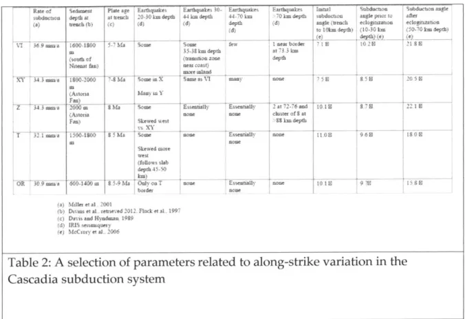
While several parameters vary along-strike in Cascadia (see Table 2),

(46)

1989), and sedimentation (Divins et al., retrieved 2012), one of the parameters that correlate best with seismic activity is slab dip (Fig 6a). Because the slab dip is shallow for the VI, X, and Y corridors to depths of 30 km, the megathrust

seismological locked and transitions zones extend eastward, the latter on to land (Fluck et al., 1997). The shallow earthquakes (33-38 km depth, Fig. 5b) near the coast correlate very well with the megathrust transition zone, and the vast majority of the intraslab activity takes place along these corridors.

The deeper earthquakes occur within the Z corridor, where a significant change in dip is accommodated. From a depth of 70 km to 110km, the dip increases within the corridor as much as 8' over a corridor-perpendicular distance of less than 50 km (McCrory et al., 2006, also see Fig. 6a and Table 2). The relationship between the earthquakes and the change in dip is perhaps less clear.

One possibility is that the change in dip is simply a result of deformation caused by the simple geometric constraints imposed by the curvature of the subduction zone (Creager and Boyd, 1991). While stresses associated with the changes could connect otherwise isolated pockets of fluid (Mibe et al., 2003, Bruhn et al., 2000) and the valley like topography formed by the changes in dip could channel fluids over a short horizontal profile, the presence of fluids would

(47)

not be required. Likewise, this interpretation would not explain differences in the Z corridor seaward of the change in dip.

Conversely, the changes in dip could be a result of the densification of the slab (Klemd et al., 2011) due to the fluid release from chlorite harzburgite in the upper mantle and subsequent triggering of the eclogitization reaction in the lower crust. This would require a fundamental difference in the incoming slab within the Z-corridor that could enable sufficient hydration of the upper mantle, such as zones of weakness associated with propagator wakes (Nedimovic et al., 2009).

The largest of these propagator wake zones includes the segment of the Z corridor imaged by this study (Fig. 6a), and also serves to delineate three very different regions of the Cascadia subduction zone. To the north, the dip of the plate is shallow, intraslab seismic activity is dense, and the 127 quaternary volcanic vents are tightly concentrated around the five major volcanoes (Mt. Meager is off the map to the north)(Hildreth, 2007). To the south, the plate dips more steeply, seismic activity is sparse, and more than 2000 quaternary vents form a near continuous array from Bumping Lake to the east of Mt. Rainier to very near the California border (Hildreth, 2007).

While most of the volcanism in the Cascades lies along the quaternary axis, there are four volcanic features within the forearc; three of them (Mt. Rainier, Mt.