HAL Id: hal-00795075
https://hal.inria.fr/hal-00795075
Submitted on 7 Aug 2019
HAL is a multi-disciplinary open access
archive for the deposit and dissemination of
sci-entific research documents, whether they are
pub-lished or not. The documents may come from
L’archive ouverte pluridisciplinaire HAL, est
destinée au dépôt et à la diffusion de documents
scientifiques de niveau recherche, publiés ou non,
émanant des établissements d’enseignement et de
Output-sensitive construction of the Delaunay
triangulation of points lying in two planes
Jean-Daniel Boissonnat, André Cerezo, Olivier Devillers, Monique Teillaud
To cite this version:
Jean-Daniel Boissonnat, André Cerezo, Olivier Devillers, Monique Teillaud. Output-sensitive
con-struction of the Delaunay triangulation of points lying in two planes.
International Journal of
Computational Geometry and Applications, World Scientific Publishing, 1996, 6 (1), pp.1-14.
�10.1142/S0218195996000022�. �hal-00795075�
OUTPUT SENSITIVE CONSTRUCTION OF
THE DELAUNAY TRIANGULATION OF
POINTS LYING IN TWO PLANES
∗
JEAN-DANIEL BOISSONNAT (Inria)
ANDR´
E C´
ER´
EZO (Univesit´
e de Nice)
OLIVIER DEVILLERS (Inria)
MONIQUE TEILLAUD (Inria)
IJCGA, Vol. 6 No. 1 (1996) 1-14
Abstract
In this paper, we propose an algorithm to compute the Delaunay tri-angulation of a set S of n points in 3-dimensional space when the points lie in 2 planes. The algorithm is output-sensitive and optimal with respect to the input and the output sizes. Its time complexity is O(n log n + t), where t is the size of the output, and the extra storage is O(n).
keywords Delaunay triangulation, Output-sensitive algorithms, Voronoi diagram, Hyperbolic distance, Computerized Tomography
1
Introduction
The Delaunay triangulation and its dual, the Voronoi diagram, are fundamental structures in computational geometry. See, for example, Refs. ( [1–3]). In two dimensions, the size of these structures, for n points, is O(n) and there exist several optimal O(n log n) algorithms for their construction. In higher dimensions, the size of the output depends on the input distribution and may vary from O(n) to O(nbd+12 c) where d denotes the dimension. In particular, in 3-dimensional space, the Delaunay triangulation of a set S of n sites may consist of a number of tetrahedra which may vary from O(n) to O(n2). Thus it
is worth seeking algorithms whose complexities depend on both the input size n and the output size t.
As is well known, constructing the Delaunay triangulation (or the Voronoi diagram) of points in d-dimensional space can be reduced to constructing a
∗This work has been supported in part by the ESPRIT Basic Research Actions No. 3075
convex hull in (d + 1)-dimensional space. Thus the output sensitive algorithm of Seidel for constructing convex hulls in higher dimensions [4] can be used to construct the Delaunay triangulation of n sites in an output sensitive manner. The time complexity of the original algorithm as described by Seidel is O(n2+ t log n) for any d ≥ 3. A recent result of Matouˇsek and Schwarzkopf [5] allows to reduce the complexity to O(n4/3+ε+ t log n) for d = 3 ; with this modification,
this algorithm is rather complicated and still not satisfying if t is o(n4/3).
Other algorithms are known that are sensitive to the output for some specific types of inputs. Incremental randomized algorithms, for instance, are sensitive to the maximal size of the successive triangulations, as in Refs. ( [6,7]). Although their time complexity may be output sensitive in some cases (in particular, if the input sites are uniformly distributed, then the triangulation is linear and the algorithms run in O(n log n) expected time), it may well happen that an intermediate triangulation is much bigger than the final one. So these algorithms are not sensitive to the size of the output in bad cases.
We previously addressed [8] the case of a set S of n points in 3-dimensional space when the points belong to a set of k given planes. We only sketch here how the algorithm works. The triangulation is constructed incrementally. Consider a tetrahedron abcd of the triangulation; the basic problem is to find the tetrahedra that share facets with it. This is equivalent to finding for each facet of abcd, say abc, the empty sphere that passes through abc and another site e(6= d). By empty sphere, we mean a sphere whose interior does not contain any of the point sites, and similarly, for short, we will say that a sphere contains a point when its interior contains that point.
In each plane P , we seek a circle which passes through a site of P , say sP, but
contains no site of P in its interior, and we report the site sP, which gives a
sphere abcsP. By comparing the k spheres obtained in this way for the k planes,
we can find the empty sphere, and so the neighbor abce of tetrahedron abcd in O(k log n) time. It follows that the overall time complexity is O(tk log n). In order to achieve an O(n) space complexity, we process the tetrahedra in an order that ensures that the union of the already constructed tetrahedra remains a topological ball at each step of the incremental construction. Such an order has been introduced by Bruggesser and Mani [9] for proving that the boundary complex of any convex polytope is shellable in any dimension. The same result has also been exploited by Seidel. [4]
Using the recent result of Matouˇsek and Schwarzkopf mentioned above, the algorithm can be extended to sets of points of Rd lying in k p-flats. [10]
Outline of the paper. In the special case of only two planes, a better algorithm can be obtained. This was known in the special case of points in 3-dimensional space constrained to lie in two parallel planes. In such a case, a deterministic algorithm has been proposed by Boissonnat, [11] whose complexity is O(n log n+ t), which is optimal with respect to the input and the output sizes.
It was shown that if we are given two sets of point sites SP and SQ lying
respectively in two parallel planes P and Q, then the three dimensional Voronoi diagram (and thus the Delaunay triangulation) of SP ∪ SQ can be obtained by
superimposing the two 2-dimensional Voronoi diagrams of SP and SQ . The
present paper is a generalization of the algorithm for two parallel planes. It will be shown in Section 4 that the situation for non parallel planes is quite similar : the 3-dimensional Delaunay triangulation can be deduced from the planar map obtained when superimposing the Voronoi diagrams of SP and SQ
for the hyperbolic metric. However, we first show in Section 3 that, using the geometric transform of Section 2, it is possible to derive more tractable (linear) diagrams that can be used instead of the hyperbolic ones.
2
The geometric transform
2.1
Circles
The correspondence between the Delaunay triangulation of a set of points in the plane and a convex hull in 3D space is well known : it is obtained by embedding the points of the plane into points of a 3-dimensional space (see Refs. ( [2, 12])). The rest of this subsection recalls the main properties of this correspondence, that will be useful in the next subsection, and for our algorithm.
Let us follow Aurenhammer’s description [12] of this embedding and recall briefly its properties, in the planar case. We can embed a given plane P into the horizontal plane of equation z = 0 of a three dimensional Euclidean space CP spanned by the coordinate axes x, y, z. The transform π maps a circle C in
P with equation C(x, y) = 0, where
C(x, y) = x2+ y2− 2ϕx − 2ψy + χ
to the non vertical plane π(C) also denoted πCof equation πC(x, y, z) = 0 where
πC(x, y, z) = z − 2ϕx − 2ψy + χ.
Here the point (ϕ, ψ) of P is the center of C and χ = C(0, 0) is the power of the origin with respect to C.
Remember that the power of a point M = (x, y) with respect to a circle C of center N and radius r is the quantity C(x, y), which is also equal to |M N |2− r2
where | · | denotes the Euclidean distance. This definition also holds for the power of a point with respect to a sphere in a three dimensional space, in fact the power of M with respect to a sphere is the power of M with respect to any circle obtained by intersecting the sphere with a plane containing M .
Let Π denote the paraboloid z = x2+ y2 in C
P . It is immediate to observe
that πC∩ Π projects vertically onto C.
The polarity ∆ with respect to Π maps a non vertical plane H : z = ax + by + c
to the point
and, more generally, a flat F to the union of the ∆(H), for H ⊇ F . Note that ∆(πC) = (ϕ, ψ, χ). In the sequel and in the figures, we will denote by C? the
point ∆(πC).
If we consider a point M as a circle of radius 0, we obtain that M?= ∆(πM)
is the vertical projection of M onto the paraboloid Π, and that πM is the plane
tangent to Π at M?.
For a point M and a non vertical plane H, M is above (in, below) H exactly if ∆(H) is above (in, below) ∆(M ).
Let us denote by SP a set of point sites in P . Let USP be the convex polyhedron, obtained by intersecting the upper half-spaces limited by all planes πM for M ∈ SP.
The preceding properties imply [12] that the Voronoi diagram of SP is the
vertical projection of USP onto P .
2.2
Pencils of circles
We first briefly recall some definitions and refer the reader to Coxeter’s [13] or Pedoes’s [14] books for example. The radical axis (also called chordale) of two circles C1 and C2 of equations Ci(x, y) = 0 (i = 1, 2) is the set of
points having the same power with respect to C1 and C2. Its equation is thus
C1(x, y) = C2(x, y). Notice that the radical axis is orthogonal to the line passing
through the two centers of the circles.
In the sequel, pencils of circles play a central role. A pencil of circles is a linear family of circles, which means that, if we denote by Ci(x, y) = 0, i = 1, 2,
the equations of two circles, the equation of any circle in the pencil will be λ1C1(x, y) + λ2C2(x, y) = 0
where λ1and λ2are constants. Any two circles of a pencil have the same radical
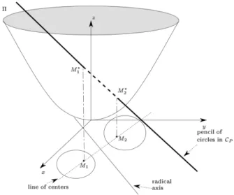
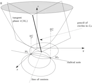
axis, called the radical axis of the pencil. The radical axis of the pencil is thus orthogonal to the line passing through all the centers of the circles of the pencil. See figures 1, 2, 3 that show different types of pencils.
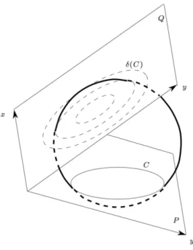
Let us now derive another consequence of the geometric transform of Sub-section 2.1. Since the mapping π is linear, a pencil of circles PCin P is mapped
by π into a pencil of planes PH in CP . Aurenhammer shows that if C and C0
are two non-concentric circles in P , then the radical axis of C and C0 is the
vertical projection of πC∩ πC0 onto P . In fact, if C and C0 are concentric, the intersection of πC and πC0 is at infinity, as well as the chordale of C and C0, so the observation still holds. For our pencil of circles PC in P , the radical axis is
thus the projection of the common line of the planes of the corresponding pencil PH in CP . This line is in fact the image by ∆ ◦ π of the pencil of circles.
The usual classification of the pencils of circles can be done in the following way. If the line representing the pencil in CP intersects the paraboloid Π in
two points, those points represent the zero-radius circles of the pencil called the limiting points of the pencil (Figure 1). If the line intersects Π in one point, the pencil is concentric (Figure 2). If the line does not intersect Π, then all the circles have two points in common, that are called the base points of the pencil.
Figure 1: A pencil of circles with limiting points
Figure 3: A pencil of circles with base points
Similarly as for spheres, we say that a circle in P is empty if it contains no point of SP in its interior. An important observation is that for a given pencil
of circles and a given set of point sites SP in P , the at most two extremal empty
circles of the pencil are the vertical projections of the intersection of USP with the line representing the pencil in CP .
These simple observations are sufficient for the purpose of this paper. A more complete presentation [15] provides a geometric interpretation of the transform of Subsection 2.1, and geometric proofs of the above facts.
3
A first algorithm
Let P and Q be two given planes and denote l = P ∩ Q their common line. SP
and SQ denote two sets of point sites lying respectively in P and Q, and we
want to compute the Delaunay triangulation of the set of points SP∪ SQ. The
choice of a circle C passing through three points a, b, c in P determines the set S of spheres intersecting P along C. The intersection of these spheres with Q is a pencil of circles in Q whose radical axis is l. Indeed, the power of a point M on l with respect to any of these circles in Q, say C0, is the power of M with respect to the sphere of S passing through C and C0, which is also the power of M with respect to the circle passing through a, b, c in P , which proves that for M in l, the power of M does not depend on the circle defined by S in Q.
So, to a point C? of C
P we can associate the line δ(C) in CQ , which is the
image by ∆ ◦ π of the associated pencil of circles in Q. Using a judicious choice of coordinates in P and Q this transformation is trivial. More precisely, we choose in both planes a system of coordinates in which the origin lies on l and
l supports the x-axis. In this way, the pencil of circles in Q determined by the point C?with coordinates (ϕ, ψ, χ) in CP is exactly the line δ(C) parallel to the
y-axis passing through the point of coordinates (ϕ, ψ, χ) in CQ . Indeed, as l is
the radical axis of the pencil, l is orthogonal to δ(C) (see Section 2 and Figure 4). Moreover, the power of the origin is constant since it is also equal to the power of the origin with respect to C.
In the sequel, CP and CQ will be identified and denoted C .
Figure 4: Case of two planes
Suppose now that abcd is a Delaunay tetrahedron. Two cases may occur : three of the vertices are in the same plane and one in the other, or there are two vertices in each plane.
In the first case, let a, b and c be the vertices in SP and d be the fourth vertex
in SQ. The intersection of P with the sphere circumscribing abcd is the circle
circumscribing abc represented in C by a vertex v of USP . The intersection of the sphere with Q is represented in C by a point that must lie on the line parallel to the y-axis and passing through v. From Section 2.2, we know that this line hits USQ in at most two points representing the possibly empty extremal circles of the corresponding pencil in Q. The (at most) two faces of USQ hit by the line
correspond to the two possible points d.
In the second case, let a, b ∈ SP and c, d ∈ SQ. For a similar reason, the
circles which are the intersection of the sphere with P and Q lie on an edge of USP and on an edge of USQ respectively. These two points of C are on the same line parallel to the y-axis.
Since all relevant lines are parallel to the y-axis, the problem can be studied in projection on a plane Π of C perpendicular to the y-axis.
At this time, it is possible to describe the algorithm. USP is computed in the coordinate system described above and is projected onto Π. We distinguish the front projection USf
P i.e. the projection of the faces of USP visible from the point (0, +∞, 0) ; and the back projection Ub
SP (as seen from (0, −∞, 0)). We can now restate the above facts. For each vertex v of USf
P or U
b
SP (which corresponds to a Delaunay circle circumscribing some triangle abc in P ) there are (at most) two possible Delaunay tetrahedra. The two points of SQ to complete
the triangle abc are represented in Π by the faces of USf
Q and U
b
SQ containing this vertex v. The previous discussion holds of course similarly for plane Q.
To each intersection of an edge e of USf P or U
b
SP (representing an empty circle in P passing through points ab) with an edge e0of USf
Q or U
b
SQ (represent-ing an empty circle in Q pass(represent-ing through points cd) corresponds the Delaunay tetrahedron abcd.
Thus the algorithm consists in superimposing the convex planar subdivisions and in constructing the four resulting subdivisions
• USfP and USf Q , • Ub SP and U f SQ , • USf P and U b SQ , • Ub SP and U b SQ .
Each of these superimpositions corresponds to the triangulation of one of the four wedges defined by the two planes. These superimpositions can be computed in time O(n + t) where n is the number of points and t the number of tetrahedra if one uses the algorithm of Guibas and Seidel [16] based on the idea of a topological sweep. [17] This complexity is optimal with respect to both the input and the output sizes.
Theorem 1. The three dimensional Delaunay triangulation of n points lying in 2 planes can be computed in O(t + n log n) time and O(n) space where t is the size of the output.
4
A second algorithm
We present in this section an intuitive way of generalizing the reconstruction algorithm [11] to the case of non parallel planes. We need first to introduce hyperbolic Voronoi diagrams.
4.1
Hyperbolic Voronoi diagrams
Let us give some hints about the hyperbolic metric (a good introduction can be found in Beardon’s book [18]) : the most classical conformal models of this two dimensional non Euclidean space are the Poincar´e upper half plane
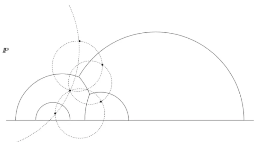
P = {x + iy ∈ C | y > 0}
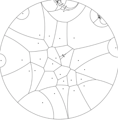
or the Poincar´e disk as in Figure 8.
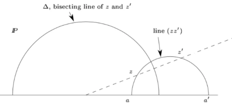
The geodesics, i.e. the hyperbolic lines, are the half-circles in P centered on the real axis (the x-axis) (exceptionally the straight half-lines parallel to the y-axis). The bisector δ of z and z0 is the upper half of the circle ∆ centered on the real axis and belonging to the pencil with limiting points z and z0 (See Figure 5).
The set of points at a given distance from a point z, that is the circle of center z in the hyperbolic sense, is a circle of the Euclidean pencil of circles defined by z as a limiting point and the real axis as radical axis. A concentric pencil of circles with center z, in the hyperbolic sense, is thus the Euclidean pencil of circles defined by z as a limiting point and the real axis as radical axis. This implies that the nearest neighbor of z among a set of sites S in P is the point of S lying on the maximal empty circle of this pencil of circles defined by z.
Figure 5: Hyperbolic lines.
One can define in the usual way the hyperbolic Voronoi diagram of a finite set S of sites in P. The cell of z ∈ S is the set of points nearer (in the hyperbolic sense) to z than to any other point in S . This is a (hyperbolically) convex
subset of P limited by arcs of bisectors. The vertices are the centers (in the hyperbolic sense) of circles passing through three sites of S , and with empty interiors: these circles are ordinary Delaunay circles of S . Notice that, for clarity, we restrict here our study to Delaunay circles entirely drawn inside
P, that is circles not intersecting l. Circles intersecting l can also be taken
into account if the hyperbolic Voronoi diagrams are properly extended. [19] Thus, apart from this restriction, the hyperbolic Voronoi diagram has the same topology as the Euclidean one, and it can be deduced from the Euclidean one by replacing the Euclidean centers of the empty circles by the hyperbolic ones, and replacing the line segments joining two vertices by hyperbolic line segments (i.e. arcs of circles).
The hyperbolic Voronoi diagram can also be obtained from USP as follows. The nearest neighbor of z is given by intersecting the convex USP with the line of C representing the circles centered at z (in the hyperbolic sense). All such lines, for all z ∈ P, have the same direction ∆ parallel to Oy, since they are associated to pencils with the same radical axis. Thus, if we project USP along the direction of ∆ onto the paraboloid Π, and then orthogonally onto P, we obtain the hyperbolic Voronoi diagram of S: in fact, the projection (parallel to ∆) of an edge of USP onto Π is the set of point-spheres equidistant (in the hyperbolic sense) from two sites of S . This gives a correspondence between the Euclidean and the hyperbolic Voronoi diagrams.
An example of such a diagram on five points is given in Figure 6. Another example of hyperbolic Voronoi diagram in the model of the Poincar´e disk is drawn in Figure 8.
4.2
The algorithm
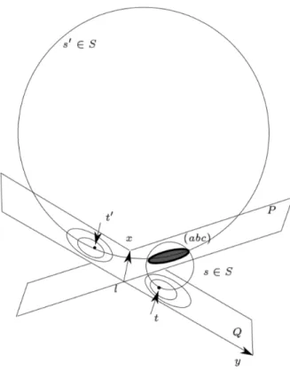
Let us use the notations defined in the preceding section and Figure 4. Suppose that abcd is a Delaunay tetrahedron, and that a, b, c lie in P . As previously noticed, the set S of spheres intersecting P along the circle abc intersects Q in a pencil of circles, denoted C, with radical axis l.
For clarity, we restrict our study to the case where the circle abc does not intersect l. Then C has two limiting points t and t0 (see Figure 7), which are determined by the two spheres s and s0 of the pencil that are tangent to Q. When we let a sphere of this pencil grow up starting from s (resp. s0), this
Figure 7: The pencil of circles C in Q
sphere will remain empty until it hits a first point d (resp. d0) of SQ. Another
way of looking for d is the following: when a, b, c are known, t can be easily obtained from the circle abc by writing that the power of O ∈ l with respect to s is also equal to the power of O with respect to the circle (abc) in P or
the power of O with respect to the circle {t} in Q. As d is given by the largest empty circle of C containing t, d is the point of SQwhich is “closest” to t in some
sense. In fact, d is exactly the nearest neighbor of t for the hyperbolic distance, and thus it can be found by locating t in the hyperbolic Voronoi diagram of SQ . Moreover, when P is rotated onto Q around l, t is nothing else than the
hyperbolic circumcenter of abc.
It follows that the Delaunay tetrahedra whose circumscribing spheres do not intersect l can be found by superimposing the hyperbolic Voronoi diagrams of SP and SQ .
By enlarging the previous discussion to tetrahedra whose circumscribing spheres intersect l, we can also compute these tetrahedra by superimposing extended hyperbolic Voronoi diagrams. [19]
This is the exact analogue of Boissonnat’s paper, [11] the hyperbolic metric being replaced by the Euclidean one when P and Q are parallel. Computing USf
P (and similarly for the other subdivisions defined in Section 3) is in fact equivalent to computing the hyperbolic Voronoi diagram of the sites in one of the half-planes of P limited by l. When P is parallel to Q the discussion can be easily adapted : pencils of circles are now concentric pencils and only one “wedge” remains relevant (the slice between P and Q).
5
Conclusion
We have shown here that the Delaunay triangulation of points lying in two planes can be computed in O(n log n + t) time, which is optimal with respect to the input and the output sizes.
This result is a further step (after the case of two parallel planes [11]) towards the efficient construction of the Delaunay triangulation in an output sensitive fashion in 3-dimensional space.
A natural application of this result is in computerized tomography, where 3D objects must be reconstructed from a series of cross-sections. The Delaunay triangulation has been shown to be a useful tool in that context but, at present, only parallel cross-sections have been considered. This is sufficient for X-ray scanners but not for other kinds of sensors (most notably ultrasonic sensors). This paper allows us to reconstruct 3D objects from non parallel cross-sections. We let as an open question whether the same bounds can be obtained if the number of planes is greater than 2; and we recall the main (and probably difficult) unsolved question in that area: is O(n log n + t) an upper bound for constructing the Delaunay triangulation of n points in d-dimensional space if the triangulation consists of t tetrahedra ?
Acknowledgments
We would like to thank Jean-Pierre Merlet for supplying us with his interactive drawing preparation system Jpdraw .
References
[1] F. P. Preparata and M. I. Shamos. Computational Geometry: an Introduc-tion. Springer-Verlag, New York, NY, 1985.
[2] H. Edelsbrunner. Algorithms in Combinatorial Geometry, volume 10 of EATCS Monographs on Theoretical Computer Science. Springer-Verlag, Heidelberg, West Germany, 1987.
[3] F. Aurenhammer. Voronoi diagrams: a survey of a fundamental geometric data structure. ACM Comput. Surv., 23:345–405, 1991.
[4] R. Seidel. Constructing higher-dimensional convex hulls at logarithmic cost per face. In Proc. 18th Annu. ACM Sympos. Theory Comput., pages 404– 413, 1986.
[5] J. Matouˇsek and O. Schwarzkopf. Linear optimization queries. In Proc. 8th Annu. ACM Sympos. Comput. Geom., pages 16–25, 1992.
[6] K. L. Clarkson and P. W. Shor. Applications of random sampling in com-putational geometry, II. Discrete Comput. Geom., 4:387–421, 1989. [7] J.-D. Boissonnat, O. Devillers, R. Schott, M. Teillaud, and M. Yvinec.
Applications of random sampling to on-line algorithms in computational geometry. Discrete Comput. Geom., 8:51–71, 1992.
[8] J.-D. Boissonnat, A. C´er´ezo, O. Devillers, and M. Teillaud. Output-sensitive construction of the 3-d Delaunay triangulation of constrained sets of points. In Proc. 3rd Canad. Conf. Comput. Geom., pages 110–113, 1991. [9] H. Bruggesser and P. Mani. Shellable decompositions of cells and spheres.
Math. Scand., 29:197–205, 1971.
[10] J.-D. Boissonnat, A. C´er´ezo, O. Devillers, and M. Teillaud. manuscript. [11] J.-D. Boissonnat. Shape reconstruction from planar cross-sections. Comput.
Vision Graph. Image Process., 44(1):1–29, October 1988.
[12] F. Aurenhammer. Power diagrams: properties, algorithms and applica-tions. SIAM J. Comput., 16:78–96, 1987.
[13] H. S. M. Coxeter. Introduction to Geometry. Wiley, New York, NY, 1961. [14] D. Pedoe. Geometry, a comprehensive course. Dover Publications, New
York, 1970.
[15] O. Devillers, S. Meiser, and M. Teillaud. The space of spheres, a geometric tool to unify duality results on Voronoi diagrams. In Proc. 4th Canad. Conf. Comput. Geom., pages 263–268, 1992.
[16] L. J. Guibas and R. Seidel. Computing convolutions by reciprocal search. Discrete Comput. Geom., 2:175–193, 1987.
[17] H. Edelsbrunner and L. J. Guibas. Topologically sweeping an arrangement. J. Comput. Syst. Sci., 38:165–194, 1989. Corrigendum in 42 (1991), 249– 251.
[18] A. F. Beardon. The Geometry of Discrete Groups. Graduate Texts in Mathematics. Springer-Verlag, 1983.
[19] A. C´er´ezo. Le plan hyperbolique `a pied, puis un bond dans l’espace. Pub-lication p´edagogique 10, Dept. Math., Nice Univ., France, 1991.