HAL Id: hal-01702391
https://hal.archives-ouvertes.fr/hal-01702391v2
Submitted on 17 Dec 2018
HAL is a multi-disciplinary open access
archive for the deposit and dissemination of
sci-entific research documents, whether they are
pub-lished or not. The documents may come from
teaching and research institutions in France or
abroad, or from public or private research centers.
L’archive ouverte pluridisciplinaire HAL, est
destinée au dépôt et à la diffusion de documents
scientifiques de niveau recherche, publiés ou non,
émanant des établissements d’enseignement et de
recherche français ou étrangers, des laboratoires
publics ou privés.
Non-isothermal compositional liquid gas Darcy flow:
formulation, soil-atmosphere boundary condition and
application to high energy geothermal simulations
Laurence Beaude, Konstantin Brenner, Simon Lopez, Roland Masson, Farid
Smaï
To cite this version:
Laurence Beaude, Konstantin Brenner, Simon Lopez, Roland Masson, Farid Smaï. Non-isothermal
compositional liquid gas Darcy flow: formulation, soil-atmosphere boundary condition and application
to high energy geothermal simulations. Computational Geosciences, Springer Verlag, In press.
�hal-01702391v2�
(will be inserted by the editor)
Non-isothermal compositional liquid gas Darcy flow: formulation,
soil-atmosphere boundary condition and application to high energy
geothermal simulations
Laurence Beaude · Konstantin Brenner · Simon Lopez ·
Roland Masson · Farid Smai
Received: date / Accepted: date
Abstract This article deals with the modelling and formulation of compositional gas liquid Darcy flow.
Our model includes an advanced boundary condition at the interface between the porous medium and the atmosphere accounting for convective mass and energy transfer, liquid evaporation and liquid outflow. The formulation is based on a fixed set of unknowns whatever the set of present phases. The thermo-dynamic equilibrium is expressed as complementarity constraints. The model and its formulation are applied to the simulation of the Bouillante high energy geothermal field in Guadeloupe characterized by a high temperature close to the surface.
Keywords Non-isothermal compositional Darcy flow; geothermal energy; soil-atmosphere boundary
condition; outflow boundary condition; porous medium drying; finite volume scheme.
1 Introduction
Geothermal energy is a carbon-free non-intermittent energy source with low environmental impact. It will contribute to the decarbonization of our economy reaching its maximum mitigation potential by 2050 [2]. In countries with a favourable geological context, high temperature geothermal energy can make a significant contribution to power production. Indeed, the world installed capacity of geothermal fields has increased of about 17 percent between 2010 and 2015 and is expected to have doubled between 2010 and 2020 [6]. As regards direct use, installed capacity growth follows the same trend [26], with a conservative assessment showing that the annual recoverable geothermal energy is in the same order as
L. Beaude
Universit´e Cˆote d’Azur, CNRS, INRIA COFFEE, Laboratoire J.A. Dieudonn´e, Parc Valrose, 06108 Nice cedex 02, France. E-mail: laurence.beaude@unice.fr
K. Brenner
Universit´e Cˆote d’Azur, CNRS, INRIA COFFEE, Laboratoire J.A. Dieudonn´e, Team Coffee, Parc Valrose, 06108 Nice cedex 02, France. E-mail: konstantin.brenner@unice.fr
S. Lopez
BRGM, scientific and Technical Center, 3 avenue Claude Guillemin, BP 36009, 45060 Orl´eans Cedex 2 France E-mail: s.lopez@brgm.fr
R. Masson
Universit´e Cˆote d’Azur, CNRS, INRIA COFFEE, Laboratoire J.A. Dieudonn´e, Team Coffee, Parc Valrose, 06108 Nice cedex 02, France. E-mail: roland.masson@unice.fr
F. Smai
BRGM, scientific and Technical Center, 3 avenue Claude Guillemin, BP 36009, 45060 Orl´eans Cedex 2 France E-mail: f.smai@brgm.fr
the world current final energy consumption [25].
The quantitative understanding of the shallow parts of geothermal systems is challenging both for the exploration and exploitation of high energy geothermal resources. First, the unsaturated zone and/or cooler superficial water flows can considerably alter evidences of the presence of a deeper geothermal resource. In some cases, the resource may be totally hidden. In terms of exploitation, as some systems underlay urbanized areas (e.g. Rotuara in New Zealand or Bouillante in the French Caribbean), resource exploitation much be carefully monitored and controlled in order to avoid unwanted induced surface manifestations or risks. Moreover, several features such as geysers, have a major cultural significance for indigenous populations and must therefore be protected and kept unaltered [34].
Numerical modelling has become essential in all phases of geothermal operations. It is used in the ex-ploration phases to assess the geothermal potential, validate conceptual hypothesis and help well siting. Field development and resource management need quantitative estimation to prevent resource exhaustion and achieve its sustainable exploitation (production/injection scenarios). Finally, numerical modelling is also helpful in studying exploitation related to industrial risks such as the interaction with shallow wa-ter levels (drinking wawa-ter resources, hydrothermal vents or eruption) (e.g. [34]). The physics embedded in the numerical model should correctly handle non-linear evolution of saturation transients with water table fluctuations, high temperature gradients and phase change processes in the shallow levels of the simulation domain.
Current software suffers several limitations in terms of boundary conditions which are known to play a major role in geothermal flows [35, 32]. Mixed-type transient boundary conditions are not supported which impedes the convenient modelling of natural processes such as recharge or seepage or water table fluctuations. Workarounds may exist (e.g. [21]) but are relatively tedious to implement and are not formu-lated in a generic way. Transient complex upper or lower boundary conditions are mandatory to take into account some crucial processes. In volcanic island settings, the inland water table may be excessively deep and the interactions between the vadose zone and the fresh water recharge may hide geothermal resources ([11], [21]). In sedimentary basins the interactions with the topography and recharge areas must be correctly taken into account to reproduce head distributions at basin scale [16]. Though many groundwater simulation software programs can deal with the vadose zone, they are rarely designed to study multiphasic hydrothermal processes. Conversely, some geothermal reservoir simulators propose to take into account a gas/air component [33] but they are still restricted to rather simple boundary condi-tions and most of the time the alternative is between fixed value/Dirichlet type for all primary variables or fixed fluxes/Neumann type for all conserved quantities (e.g. [36]).
The objective of this work is to investigate a new formulation for non-isothermal compositional gas liquid Darcy flows and to couple it with an advanced soil-atmosphere boundary condition. The composi-tional model should typically account for the water component which can vaporize into the gas phase and for a set of gaseous components which can dissolve into the liquid phase. The soil-atmosphere boundary condition, based on mole and energy balance equations set at the interface, should take into account the vaporization of the liquid phase in the atmosphere, the convective molar and energy transfer, a liquid outflow condition as well as the precipitation recharge and the heat radiation.
Different formulations have been studied for isothermal and non-isothermal compositional Darcy flows. They basically differ by their choice of the principal unknowns and equations and by the way they deal with phase transitions, which is one of the main difficulty of this type of models. The objective of such a choice is usually to reduce the non-linearity of the successive non-linear systems that typically arise when solving a transient problem with an Euler fully implicit time integration scheme.
Let us distinguish between variable switch and persistent variable formulations. The first ones adapt the set of principal unknowns and equations to the set of present phases which can vary in space and time.
The most well known formulation in this family is the so called natural variable or Coats’ formulation widely used in reservoir simulations [14, 13, 19, 42]. It has the advantage to use the physical variables of the thermodynamic and hydrodynamic laws as the set of principal unknowns. Its main drawback is to require a cumbersome switch of this set of variables depending on the set of present phases at each point of the space time domain. On the other hand, persistent variable formulations are based either on natural physical quantities such as overall component molar fractions or total specific enthalpy (see [41]), or alternatively on nonstandard principal unknowns such as in [8, 27]. Another strategy to avoid the switch of variables is based on the extension of some physical quantities such as the phase molar fractions like in [23] using component fugacities, or the phase molar fractions and pressures like in [3, 28]. Let us also mention the negative saturation formulations [1, 37] belonging to this family. A comparison between some of these formulations can be found in [41, 28] in the case of isothermal compositional Darcy flows. Our choice of the formulation is based, like in the Coats’ formulation, on the phase pressures, phase saturations, temperature and phase molar fractions as set of principal unknowns. This is a convenient choice since all the physical laws can be directly expressed using subsets of this set of variables. It is also a very natural choice in single phase regions which are usually dominant in geothermal applications. In order to avoid the switch of variables, this choice of the principal unknowns is combined with an exten-sion of the phase molar fractions of an absent phase by the molar fractions at thermodynamic equilibrium with the present phase. It results that the set of principal unknowns does not depend on the set of present phases. Moreover, the phase transitions can be expressed as complementarity constraints as in [23] which means that the non-linear systems can be solved using semi-smoothed Newton techniques such as the Newton-min algorithm [22, 5]. This formulation has been preferred to the formulation proposed in [23] since the use of the component fugacities as principal unknowns rather than the phase molar fractions results in additional non-linear couplings between the molar fractions and the temperature which are not desirable for non-isothermal Darcy flows. In this work, the efficiency of this formulation combined with different improvements of the Newton-min non-linear solver will be investigated on several test cases. It will also be compared in terms of non-linear convergence with the formulation proposed in [23] over one simulation.
As mentioned in [35, 32], the interaction between the flow in the porous medium and the atmosphere plays an important role in geothermal flows. Since the coupling between the porous medium and surface flows is not computationally realistic at the space and time scales of a geothermal flow, our objective is rather to model the soil-atmosphere interaction using an advanced boundary condition accounting for the matter (mole) and energy balance at the interface between the porous medium and the atmosphere. Such model should consider the vaporization of the liquid phase, the convective molar and energy transfer, a liquid outflow condition at seepage surfaces, as well as the heat radiation and the precipitation influx.
Assuming the vaporization of the liquid phase at the soil-atmosphere interface, the molar and energy normal fluxes at the interface on the atmosphere side are frequently approximated in hydrogeology by two-point fluxes between the gas phase at the interface and the atmosphere at a reference height [15, 12]. The transmissivities of these two-point fluxes are based on convective molar and energy transfer coefficients. Such approximation basically assumes that the lateral variations in wind, air temperature and humidity can be neglected [40]. Let us refer to the textbook [30] on meteorology for the compu-tation of convective molar and energy transfer coefficients at the soil-atmosphere interface depending on the roughness of the soil surface including the effect of the vegetation, on the wind velocity, on the eddy diffusivity in the air stream and stability of the air above the heated soil surface. The radiation which is absorbed by and emitted from the soil surface as well as the precipitation recharge can also be incorporated in such models [15, 12].
Outflow boundary conditions are frequently used in hydrogeology at seepage surfaces allowing the groundwater discharge to occur where the water table intercepts a sloping land surface. They have already been used for geothermal applications as in [21] for a single component liquid gas Darcy flow model. For the Richards equation, outflow boundary conditions are modelled by complementarity constraints between the non negative liquid normal flux and the non negative capillary pressure (see [39]). For liquid
gas Darcy flow models, they are combined with a Dirichlet boundary condition for the gas pressure [24]. To our knowledge, their extension to general non-isothermal compositional liquid gas Darcy flows has not yet been derived.
In this work, both the evaporation and liquid outflow models are combined in a single boundary condition which automatically switches from evaporation to evaporation and liquid outflow boundary condition. It assumes that the liquid phase does not accumulate at the surface on the atmosphere side, considering that standing water condition such as lake or sea can easily be expressed in the form of Dirichlet conditions. Alternatively, one would need to model the flow of the liquid phase at the soil-atmosphere surface which has not been considered here and might induce a coupling with a system with different time scales than the underlying geothermal system. Our boundary condition is coupled with the general non-isothermal compositional liquid gas Darcy flow model. The previous formulation of the Darcy flow model is adapted to account for the new unknowns and equations at the soil-atmosphere in-terface. The derivation of the two-point molar and energy fluxes in the atmosphere is obtained starting from the transmission conditions proposed in [31] (see also [29, 40]) for the coupling of non-isothermal compositional liquid gas Darcy and free gas flows. The complementarity constraint for the liquid outflow is extended to non-isothermal compositional flows using a switching criterion based on the thermody-namic equilibrium between the gas and liquid phases at the interface on the free-flow side.
The structure of the rest of this article is as follows. The non-isothermal compositional two-phase Darcy flow model and its formulation are presented in Section 2. The soil-atmosphere boundary condition is derived in Section 3. Then, the finite volume two-point flux discretization of the model as well as the Newton-min algorithms used to solve the fully coupled systems at each time step of the simulation are introduced in Section 4. The convergence of the model is then studied over a semi-analytical 1D stationary solution in Section 5. In Section 6, the soil-atmosphere evaporation boundary condition is compared with a full-dimensional free gas flow and transport model coupled to the liquid gas Darcy flow. In Section 7, the model and its formulation are studied numerically in terms of solution and convergence of the Newton-min non-linear solvers on several geothermal test cases including 1D test cases and 2D cuts of the Bouillante geothermal field in Guadeloupe.
2 Non-isothermal compositional two-phase Darcy flow model
We consider a non-isothermal compositional liquid gas Darcy flow model withP = {g,l} denoting the
set of gas and liquid phases. Each phaseα∈ P is a mixture of a set of components denoted by C
includ-ing typically a water component, denoted w, which can vaporize in the gas phase and a set of gaseous
components which can dissolve in the liquid phase. The thermodynamic properties of each phaseα∈ P
depend on its pressure Pα, the local equilibrium temperature of the system T and its molar fractions
Cα= (Ciα)i∈C.
For each phaseα ∈ P, we denote byζα(Pα, T,Cα) its molar density, by ρα(Pα, T,Cα) its mass density, by µα(Pα, T,Cα) its dynamic viscosity, by eα(Pα, T,Cα) its molar internal energy and by hα(Pα, T,Cα) its molar enthalpy. For the gas phase, assuming an ideal mixture, the molar enthalpy is defined by
hg(Pg, T,Cg) =
∑
i∈C
Cighgi(Pg, T ), (2.1)
where hgi(Pg, T ) is the molar enthalpy of the component i in the gas phase. Thermodynamic equilibrium
between the gas and liquid phases is assumed for each component and governed by the phase fugacities denoted by fα(Pα, T,Cα) = ( fiα(Pα, T,Cα))i∈C,α∈ P.
The rock porosity is denoted byϕ(x) and the rock permeability tensor byΛΛΛ(x) where x denotes
the spatial coordinates. The hydrodynamic Darcy laws are characterized by the relative permeability kαr(x, Sα) of each phaseα∈ P, as a function of the phase saturation Sα, and by the capillary pressure
Pc(x, Sg) = Pg− Pl. The relative permeabilities and capillary pressure are piecewise constant for each
rocktype, thus their dependence on x is omitted in the following for the sake of simplicity.
Our formulation of the model (called T-PSC in the following) is based on the fixed set of unknowns defined by X = ( Pα, T, Sα,Cα,α∈ P ) . (2.2)
Note that, as opposed to the Coats’ variable switch formulation [14, 13, 19, 42], the molar fractions Cα of an absent phaseα are extended by the ones at equilibrium with the present phase in the sense that the equality of the gas and liquid fugacities fg(Pg, T,Cg) = fl(Pl, T,Cl) always holds.
Let ni(X ) be the number of moles of the component i∈ C per unit pore volume defined by
ni(X ) =
∑
α∈Pζ α
SαCiα, i∈ C .
We introduce the rock energy per unit rock volume defined by Er(T ) and the fluid energy per unit pore
volume defined by
E(X ) =
∑
α∈Pζ αSαeα.
Let us denote by g the gravitational acceleration vector. The generalized Darcy velocity of the phase
α∈ P is given by Vα=−k α r µαΛΛΛ(x) ( ∇Pα−ραg ) . (2.3)
The total molar flux of the component i∈ C is denoted by qiand the energy flux by qe, with
qi=
∑
α∈P
Cαi ζαVα, qe=
∑
α∈P
hαζαVα−λ∇T, (2.4)
whereλ stands for the bulk thermal conductivity of the fluid and rock mixture.
The system of equations accounts for the molar conservation of each component i∈ C together with
the energy conservation
ϕ(x)∂tni+ div(qi) = 0, i∈ C ,
ϕ(x)∂tE + (1−ϕ(x))∂tEr+ div(qe) = 0. (2.5)
It is complemented by the following capillary relation between the two phase pressures and the pore volume balance { Pc(Sg) = Pg− Pl, ∑ α∈PS α= 1. (2.6)
In the spirit of [23, 28], the liquid gas thermodynamic equilibrium can be expressed as the following
complementarity constraint for each phase α ∈ P combined with the equality of the gas and liquid
fugacities of each component { Sα≥ 0, 1 − ∑ i∈CC α i ≥ 0, Sα(1− ∑ i∈CC α i ) = 0, α∈ P, fig(Pg, T,Cg) = fl i(Pl, T,Cl), i∈ C . (2.7)
Note that our formulation of the model leads, independently on the set of present phases, to the
fix sets of 2#C + 5 unknowns (2.2) and of 2#C + 5 equations (2.5)-(2.6)-(2.7) including the #C + 1
conservation equations (2.5) and the remaining #C + 4 local closure laws (2.6)-(2.7). It also has the
advantage to express the thermodynamic equilibrium as complementarity constraints which will allow the use of semi-smooth Newton methods [22, 5] to solve the non-linear systems at each time step of the simulation as specified in Section 4.1.
3 Soil-atmosphere boundary condition for non-isothermal compositional liquid gas Darcy flow The fluid and energy transport in high energy geothermal systems is deeply governed by the conditions set at the boundary of the computational domain. In particular, it is well known that the modelling of the interaction between the porous medium model and the atmosphere plays an important role [35, 32]. In this section, a boundary condition is derived to model the soil-atmosphere interaction based on mole and energy balance equations set at the interface. The model takes into account two coupling processes: on the one hand, the vaporization of the liquid phase and the convective molar and energy transfer in the atmosphere described in Subsection 3.1, on the other hand, a liquid outflow condition described in Subsection 3.2. Both coupling processes will be combined in a single boundary condition assuming that the liquid phase does not accumulate at the surface. The radiation and the precipitation recharge are also considered.
3.1 Convective molar and energy transfer in the atmosphere
3.1.1 Transmission conditions at the interface between a non-isothermal compositional liquid gas Darcy flow and a gas free flow
The derivation of the boundary condition accounting for convective molar and energy transfer in the atmosphere can be explained starting from the transmission conditions introduced in [31] (see also [29, 40]) to couple a non-isothermal compositional liquid gas Darcy flow with a gas free flow. These con-ditions state the continuity of the component molar and energy normal fluxes, assuming instantaneous vaporization of the liquid phase, as well as the continuity of the gas molar fractions, of the temperature and of the gas pressure, neglecting the gas pressure jump. It is complemented by the thermodynamic equilibrium between the liquid and gas phases and by the Beavers-Joseph condition. On the free-flow side, the component molar and energy fluxes are defined by
wi=ζg(P, T,C) ( Ciu− Dt∇Ci ) , i∈ C , we=ζg(P, T,C)hg(P, T,C)u−λt∇T −
∑
i∈Cζ g(P, T,C)hg i(P, T )Dt∇Ci, (3.1)where u denotes the gas velocity, P the pressure, C = (Ci)i∈C the gas molar fractions, T the temperature,
Dtthe turbulent diffusivity andλtthe turbulent thermal conductivity. The continuity of the component
molar normal fluxes states that
wi· n = qi· n, i ∈ C , (3.2)
where the unit normal vector n at the interface is oriented outward from the porous medium domain. The last term in the free-flow energy flux in (3.1) introduces a strong non-linear coupling between the component molar and energy fluxes which raises an additional difficulty in the two-point approximation of the normal fluxes. This can be addressed in a simple and efficient way if the dissolution of the gaseous components in the liquid phase is small which corresponds to the usual case. In such a case, using
ζg<<ζl, C
w<< 1,∑i∈CCi= 1 and (3.2), we can derive that
|qi· n| << |qw· n| ∼ζg|u · n| ∼ζgDt|∇Cw· n|, (3.3)
for all i∈ C \ {w}. Using that ∑i∈CCi= 1, one has
(we+λt∇T) · n =ζg(P, T,C) ( hg(P, T,C)u· n −
∑
i∈C hgi(P, T )Dt∇Ci· n ) =ζg(P, T,C) (∑
i∈C hgi(P, T )Ciu· n −∑
i∈C \{w} (hgi(P, T )− hgw(P, T ))Dt∇Ci· n ) = hgw(P, T )ζg(P, T,C)u· n +∑
i∈C \{w} (hgi(P, T )− hgw(P, T ))wi· n. (3.4)From (3.3) and (3.2), it results that
(we+λt∇T) · n ∼ hgw(P, T )ζg(P, T,C)u· n,
allowing the following approximation of we· n
ewe· n = hgw(P, T )ζg(P, T,C)u· n −λt∇T · n. (3.5)
3.1.2 Two-point flux approximation
The boundary conditions are obtained by two-point flux approximations of the component normal fluxes wi· n, i ∈ C and of the energy normal flux ewe· n. These two-point fluxes are computed between the
interface on the atmosphere side and the far field atmospheric conditions at a given reference height. The far field atmospheric conditions are defined by the constant gas molar fractions C∞g,atm, temperature T∞atm
and pressure Patm, which fixes the far field atmospheric specific gas enthalpy of the water component
hg,atmw,∞ = hgw(Patm, T∞atm). From the transmission conditions stated above, the temperature, the gas molar
fractions and the gas pressure defined at the interface on the atmospheric side, match with their values
on the porous medium side and consequently they are denoted respectively by T , Cgand Pg. The
two-point flux approximations account for the turbulent boundary layers of the gas flow and transport in the atmosphere using the molar and energy transfer coefficients Hmand HT. These coefficients are usually
obtained from correlations used for environmental gas flows depending on the roughness of the soil surface including the effect of the vegetation, on the wind velocity, on the eddy diffusivity in the air stream and stability of the air above the heated soil surface [30]. The two-point fluxes also take into account the convective normal fluxes using, as additional unknown, the gas molar flow rate qg,atmat the interface on the atmosphere side oriented outward from the porous medium domain. It is combined with an upwinding of the gas molar fractions and of the gas enthalpy of the water component between the interface and the far field atmospheric conditions. This leads us to define the following two-point fluxes oriented outward from the porous medium domain
qg,atmi = (qg,atm)+Cig− (qg,atm)−Cg,atmi,∞ + Hm
(
Cig−Cg,atmi,∞ )
, i∈ C ,
qg,atme = (qg,atm)+hgw(Pg, T )− (qg,atm)−hg,atmw,∞ + HT(T− T∞atm), (3.6)
where for any real u, we have set (u)+= max(0, u) and (u)−= max(0,−u).
Neglecting the variations of pressure in the atmosphere leads to the following continuity equation for the gas pressure
Pg= Patm. (3.7)
Thermodynamic equilibrium is always assumed at the interface in the sense that the gas molar fractions and pressure at the interface on the porous medium side are extended by the one at equilibrium with the liquid phase in the absence of the gas phase. On the other hand, the liquid phase can appear or disappear according to the liquid phase complementarity constraint. It results that the following equations hold at the interface fig(Pg, T,Cg) = fl i(Pl, T,Cl), i∈ C , ∑ i∈CC g i = 1, Sl≥ 0, 1 − ∑ i∈CC l i≥ 0, Sl(1− ∑ i∈CC l i) = 0, Sg=Sg(Pg− Pl), ∑ α∈PS α= 1, (3.8)
where Pl is the liquid pressure, Cl the liquid molar fractions and Sα,α ∈ P the saturations at the
the capillary pressure function Pc(Sg). As detailed in [9, 10] and in Subsection 7.1.2, a switch of variables
between Sgand Pccould also be used in order to account for non invertible capillary functions.
Regarding the interface energy balance, the model can also account for the solar and long wave radiation that is absorbed by and emitted from the soil surface defined by the following net radiation Rn
( W. m−2)
Rn= (1− a)Rs+ Ra−εσSBT4, (3.9)
where Ra( W. m−2) is the incoming long-wave radiation emitted by the atmosphere, Rs( W. m−2) is the
net short-wave radiation, a is the surface albedo,σSB( W. m−2. K−4) is the Stephan-Boltzmann constant
andεthe soil emissivity.
3.2 Liquid outflow complementarity constraint
The liquid phase is assumed to vaporize instantaneously when leaving the porous medium as long as the atmosphere is not saturated with water vapour. As soon as the atmosphere is vapour saturated at the interface, the component molar and energy normal fluxes in the liquid phase defined by
ql,atmi = Cil,atmql,atm, i∈ C ,
ql,atme = hl(Pl, T,Cl,atm)ql,atm, (3.10)
are allowed to exit the porous medium, where ql,atm≥ 0 is an additional unknown corresponding to the
total liquid molar flow rate oriented positively outward to the porous medium domain. It is assumed that the liquid phase does not accumulate at the surface on the atmosphere side, because modelling the flow of the liquid phase at the soil-atmosphere surface might induce a coupling with a system with different time scales than the underlying geothermal system. Moreover, the accumulation of water such as lake or sea can easily be expressed in the form of Dirichlet conditions. In (3.10), the liquid molar fractions Cl,atm= (Cl,atm
i )i∈Cat the interface on the atmosphere side are those at thermodynamic equilibrium with
the gas phase thus are such that
fl(Patm, T,Cl,atm) = fg(Pg, T,Cg). (3.11)
Note that, due to the jump of the capillary pressure which vanishes on the atmosphere side, Cl,atmdoes not match in general with the liquid molar fractions on the porous medium side Clwhich satisfies
fl(Pl, T,Cl) = fg(Pg, T,Cg). (3.12)
The liquid molar outflow rate ql,atmis determined by the following complementarity constraint
account-ing for the thermodynamic equilibrium between the liquid and gas phases at the interface on the atmo-sphere side (1− ∑ i∈CC l,atm i ) ql,atm= 0, 1− ∑ i∈CC l,atm i ⩾ 0, ql,atm⩾ 0. (3.13)
It remains to eliminate the liquid molar fractions Cl,atmfrom (3.10) and (3.13). Let us consider for f∈ RC the functionCl( f , Pl, T )∈ RC defined as the unique solution of the equation fl(Pl, T,Cl) = f .
From fg(Pg, T,Cg) = fl(Pg, T,Cl,atm) = fl(Pl, T,Cl) := ¯f given by the equations (3.11) and (3.12), it
results that
On the one hand, if Sl> 0, it follows that 1−
∑
i∈C Cil,atm=∑
i∈C ( Cli−Cil,atm ) =∑
i∈C ( Cl i( ¯f , Pl, T )− Cli( ¯f , Pg, T ) ) . (3.14)Following [28], since the function∑i∈CCl
i( f , P, T ) is strictly decreasing with respect to P, it results that
the complementarity constraint (3.13) is equivalent to {
(Pg− Pl) ql,atm= 0,
Pg− Pl⩾ 0, ql,atm⩾ 0. (3.15)
On the other hand, if Sl= 0 then one has Pg− Pl= Pc(1) > 0 and∑i∈CCil,atm< 1. It results that both
conditions (3.15) and (3.13) imply that ql,atm= 0. Finally, let us remark that if (3.15) holds, the liquid outflow fluxes in (3.10) rewrite as follows
ql,atmi = Cilql,atm, i∈ C ,
ql,atme = hl(Pl, T,Cl)ql,atm. (3.16)
The model also takes into account the following component molar and energy flow rates which represent the precipitation recharge
ql,raini = Cil,rainql,rain, i∈ C , ql,raine = hl(Patm, T∞atm,Cl,rain)ql,rain,
(3.17)
with the rain molar fractions denoted by Cl,rain= (Cl,rain
i )i∈C, a temperature assumed at equilibrium
with the far field atmosphere, the rain molar enthalpy denoted by hl,rain= hl(Patm, Tatm
∞ ,Cl,rain) and a
non positive rain molar flow rate ql,rain≤ 0.
3.3 Evaporation-outflow boundary condition
Both the liquid outflow and evaporation models are combined in a single boundary condition, assuming that the liquid does not accumulate at the surface. Gathering the equations (3.6), (3.7), (3.8), (3.15), (3.16), (3.17) together with the component molar an energy balance equations, the evaporation-outflow boundary condition at the interface is defined by the sets of 7 + 2#C unknowns
XΓ =
(
qg,atm, ql,atm, T, Pα, Sα,Cα,α∈ P )
and equations qi· n = (qg,atm)+Cig− (qg,atm)−C g,atm i,∞ + Hm ( Cig−Cg,atmi,∞ ) +Cl iql,atm+C l,rain i ql,rain, i∈ C ,
qe· n = (qg,atm)+hgw(Pg, T )− (qg,atm)−hg,atmw,∞ + HT(T− T∞atm)
−Rn+ hl(Pl, T,Cl)ql,atm+ hl,rainql,rain,
Pg= Patm, Sg=Sg(Pg− Pl), ∑ α∈PS α= 1, ∑ i∈CC g i = 1, min ( Sl, 1− ∑ i∈CC l i ) = 0, fig(Pg, T,Cg) = fil(Pl, T,Cl), i∈ C min ( Pg− Pl, ql,atm ) = 0. (3.18)
4 Discretization and non-linear solvers
The system of equations (2.5)-(2.6)-(2.7)-(3.18) is discretized using a finite volume discretization in space with a Two-Point Flux Approximation (TPFA) of the Darcy and Fourier fluxes [18, 17] combined with a phase based upwind scheme for the approximation of the mobilities [4, 18, 20]. A mesh satisfying the admissibility condition of TPFA schemes at both inner and boundary faces is used [18, 17]. It can be typically a triangular mesh with acute angles and isotropic permeability, a Voronoi mesh with isotropic permeability or a Cartesian mesh with anisotropic permeability aligned with the axes. In all cases the permeability is assumed cellwise constant.
LetΩ denote a bounded polytopal domain ofRd(polygonal for d = 2 or polyhedral for d = 3) and
Γ⊂∂Ωthe boundary on which the soil-atmosphere evaporation-outflow boundary condition is imposed.
Let us denote byM the set of cells that are disjoint open polytopal subsets ofΩ such that∪K∈MK =Ω. It is assumed that there exists a subsetFΓ of the set of faces such that
Γ = ∪
σ∈FΓ
σ.
For the sake of simplicity only the boundary facesσ ∈ FΓ are considered in the following. The time
integration is based on a fully implicit Euler scheme to avoid severe restrictions on the time steps. For N∈ N∗, let us consider the time discretization t0= 0 < t1<··· < tn−1< tn<··· < tN = t
f of the time
interval [0,tf]. We denote the time steps by∆tn= tn−tn−1for all n = 1,··· ,N.
Let us denote the set of physical unknowns by
XK=
(
PKα, TK, SαK,CKα,α∈ P
)
, (4.1)
for each cell K∈ M and by
Xσ=
(
qg,atmσ , ql,atmσ , Pσα, Tσ, Sασ,Cασ,α∈ P )
, (4.2)
for each boundary faceσ∈ FΓ. The full set of unknowns is denoted by
For each degree of freedom ν ∈ M ∪ FΓ, we denote by Rν(XD) the residual vector (
Rν,i(XD), i∈ C ∪{e})of the component and energy conservation equations and byLν(Xν) the residual vector of the local closure laws. It defines the following non-linear system at each time step n = 1, ..., N
0 =R(XD) = ( RK(XD) LK(XK) ) K∈ M , ( Rσ(XD) Lσ(Xσ) ) σ∈ FΓ, (4.4)
where the current time step superscript n has been dropped.
4.1 Newton-min non-linear solver
The non-linear systemR(XD) = 0 is solved using a Newton-min solver [22, 5] as detailed below. In order
to reduce the size of the linear systems to be solved at each Newton-min iteration to #C + 1 equations
and unknowns for each degree of freedomν∈ M ∪FΓ, the set of unknowns Xνis split into #C +1
pri-mary unknowns Xνpand the remaining secondary unknowns Xs
ν. This splitting is done for each degree of
freedom in such a way that the Jacobian of the local closure laws∂L∂Xνs
ν(Xν) with respect to the secondary
unknowns is non singular.
The Newton-min algorithm is initialized with an initial guess XD(0)usually given by the previous time step solution and iterates on the following steps for r = 0,··· , until the following stopping criterion is satisfied max i∈C ∪{e} ∑ ν∈M ∪FΓ |Rν,i(XD(r))| ∑ ν∈M ∪FΓ |Rν,i(XD(0))| ≤εR or dim(X )
∑
i=1 max ν∈M|dX (r) ν,i| ∆Xi + dim(XΓ)∑
i=1 max ν∈FΓ|dX (r) ν,i| ∆Xi ≤εX with dXν,i(r)= {dXν,ip (r) if i is a primary unknown, dXν,is (r) if i is a secondary unknown.
andεR= 10−8,εX= 10−6, given∆Xi> 0, i = 1,··· ,dim(Xν) and with the Newton’s steps dXν,is (r), dXν,ip (r)
defined respectively in (4.5) and (4.6). If the convergence it not met after rmaxNewton iterations, the time
step is chopped.
1. Computation of the residualR(XD(r)) and of the Jacobian matrix with elimination of the secondary unknowns. It starts with the choice of the primary and secondary unknowns for each degree of
free-domν ∈ M ∪ FΓ depending only on the active complementarity constraints, choice specified in
Table (4.1). Then the matrices Asp (r)ν and the vectors Bs (r)ν ,ν∈ M ∪ FΓ defined by
Asp (r)ν =− ( ∂Lν ∂Xνs (r) )−1 ∂Lν ∂Xνp (r) , Bs (r)ν = ( ∂Lν ∂Xνs (r) )−1 Lν, and such that
are computed to obtain the reduced Jacobian J(r)= (Jν,ν(r)′)(ν,ν′)∈(M ∪F
Γ)2 defined by the square
ma-trices of size #C + 1 Jν,ν(r)′= ∂Rν ∂Xνp (r)′ (XD(r)) + ∂Rν ∂Xνs (r)′ (XD(r))Asp (r)ν′ ,
and the reduced right hand side B(r)= (B(r)ν )ν∈M ∪FΓ defined by the vectors of size #C + 1 B(r)ν =−Rν(XD(r))−
∑
ν′∈M ∪FΓ
∂Rν
∂Xνs (r)′
(XD(r))Bs (r)ν′ . 2. Computation of the solution of the reduced linear system
J(r)dXDp (r)= B(r). (4.6) 3. Update of the unknowns Xν(r),ν∈ M ∪ FΓ with a possible relaxationθ(r)∈ (0,1]
{ Xνp (r+1)= Xνp (r)+θ(r)dXνp (r), Xνs (r+1)= Xνs (r)+θ(r) ( Asp (r)ν dXνp (r)+ Bs (r)ν ) . (4.7)
4. Additional updates of some unknowns in order to satisfy exactly some non-linear closure laws to be specified.
The step 4 of the above algorithm allows proposing different improvements of the basic Newton-min algorithm that are detailed in the following paragraphs.
Table 4.1 Choice of the primary unknowns of the degree of freedomν∈ M ∪ FΓ depending on the active complementarity constraints of the Newton-min algorithm.
ν∈ FΓ ν∈ M
ql,atmν = 0
qg,atmν , Pc,ν, (Cl
i,ν)i=1,#C −1 1− ∑i∈CC g i,ν= 0 Pνg, Sgν, (Cl i,ν)i=1,#C −1 1− ∑ i∈CC l i,ν= 0 1− ∑ i∈CC l i,ν= 0 Pνg− Pl ν= 0 qg,atmν , ql,atmν , Tν, Sgν= 0 Pνg, Tν, (Cl i,ν)i=1,#C −1 1− ∑ i∈CC l
i,ν= 0 (Ci,νl )i=1,#C −2 1− ∑
i∈CC l i,ν= 0 ql,atmν = 0 qg,atmν , Tν, (Ci,gν)i=1,#C −1 1− ∑i∈CC g i,ν= 0 Pνg, Tν, (Ci,νg )i=1,#C −1 Sl ν= 0 Slν= 0
4.1.1 Basic Newton-min algorithm
The basic version of the Newton-min algorithm only enforces at each iterate the following non-linear
closure law forν∈ M ∪ FΓ
Pνg− Pνl = Pc(Sgν).
Our objective for this basic Newton-min algorithm was to use no projections of the physical unknowns onto their physical bounds. However, in order to obtain the convergence of the Newton-min algorithm, it was necessary to project the molar fractions of a present phase within the range say [−0.2;1.2] at each Newton iterate.
4.1.2 Newton-min with projection on the complementarity constraints
In order to obtain a better convergence of the Newton-min algorithm, all the complementarity constraints of type min(X1, X2) = 0 are enforced at the initial guess and at each Newton iterate. In addition, Pνg−Pνl=
Pc(Sgν) is also enforced at each Newton iterate and the following physical ranges are imposed on the molar
fractions of a present phase and on the saturations if Sαν > 0 then 0≤ Ci,αν≤ 1, i ∈ C , α∈ P, Sαν ⩾ 0, α∈ P, ∑ α∈PS α ν = 1.
An additional improvement also studied in the numerical section is to test the appearance of a missing phase using the molar fractions at equilibrium with the present phase rather than their linear Newton updates.
4.1.3 Newton-min with projection on the complementarity constraints and thermodynamic equilibrium
In addition to the previous updates, the molar fractions Cα¯ which are secondary unknowns (see
Ta-ble 4.1), complemented by the temperature if both phases are present, are updated in order to verify the following closure laws at each Newton iterate
min ( Sαν¯, 1− ∑ i∈CC ¯ α i,ν ) = 0, fig(Pνg, Tν,Cνg) = fil(Pνl, Tν,Cνl), i∈ C
for allν∈ M ∪FΓ. Note that the first equation is already satisfied if only one phase is present as Sαν¯= 0.
5 Convergence of the Finite Volume scheme to a semi-analytical 1D stationary solution
In this section, a simplified 1D non-isothermal liquid gas model with a single water component is used to analyse the convergence of the TPFA scheme with the T-PSC formulation to a semi-analytical stationary solution.
Let us consider a single water component (C = {w}) liquid gas non-isothermal Darcy flow model on
the 1D domainΩ= (z0, z3), z3> z0. Let us assume constant liquid and gas molar densitiesζlandζg, and
viscositiesµlandµg. The liquid and gas molar enthalpies are defined by hα(T ) = cαpT ,α∈ P, with the molar heat capacities cgp> clp. Let us denote by Psat(T ) the saturated vapour pressure and by Tsat(P) its
inverse. The thermal conductivity is assumed constantλ> 0. The relative permeabilities krα(Sα),α= l, g are such that kαr(0) = 0 and krα(1) = 1. The capillary pressure is neglected. The absolute permeability of the porous mediumΛΛΛ is also assumed constant.
Let us recall the definition of the water (or total) molar flow rate qw=ζlVl+ζgVg,
with Vα=−kαr(Sα)
µα ΛΛΛ∂z(P +ρα|g|z) andρα=ζαmw where mwdenotes the water molar mass. We also
set S = Sg= 1− Sl. The energy flow rate is
The stationary solution P(z), T (z), S(z), z∈Ω is such that ∂zqw= 0, ∂zqe= 0 and Pg= Psat(T ), if 0 < S < 1, Pg≥ P sat(T ), if S = 0, Pg≤ P sat(T ), if S = 1.
The boundary conditions specify at the bottom boundary z = z0 the input saturation S = 0, the input
molar flow rate qw,0> 0 and the input energy flow rate qe,0. The temperature at z = z0is denoted by T0
and the pressure by P0. It is assumed that P0> Psat(T0) meaning that only the liquid phase is present at
the bottom boundary. At the top boundary we impose a gaseous state of temperature T3and pressure P3
which are such that P3< Psat(T3).
We assume that the solution has three zones defined by z0< z1< z2< z3and such that S = 0 on
(z0, z1), S = 1 on (z2, z3) and P = Psat(T ) on (z1, z2).
Let us denote by Pi, Tithe pressure and temperature at z = zi for i = 0, 1, 2, 3. The saturation S1at
point z1is continuous and equal to S1= 0. At point z2the saturation may be discontinuous with S+2 = 1
and S−2 to be determined.
We define the following set of 8 unknowns U = (P0, T0, P1, T1, P2, T2, z1, z2) for which we are going
to define 8 equations. Since S = 0 on [z0, z1], qw,0=−ζ l µlΛΛΛ∂z(P +ρ l|g|z).
Integrating this equation between z0and z1, we obtain
P1− P0=−(ρl|g| +µ lq w,0 ζlΛΛΛ )(z1− z0). Moreover,∂zqe= 0 gives al∂zT =∂z2T with al= clpqw,0 λ ,
from which we deduce that
T (z) = El+ Dlealz, with αl i = ea lz i, i = 0, 1, El=α l 1T0−α0lT1 αl 1−α0l , Dl= T1− T0 αl 1−α0l . Introducing this formula into
qe,0= clpT qw,0−λ∂zT,
we get
qe,0= clpElqw,0+ Dlea
lz
(clpqw,0−λal) = clpqw,0El.
Likewise on ]z2, z3], we have S = 1 from which we deduce that
P3− P2=−(ρg|g| +µ gq w,0 ζgΛΛΛ )(z3− z2) and T (z) = E g+ Dgeagz, with ag=c g pqw,0 λ , α g i = e agzi, i = 2, 3, Eg=α g 3T2−α2gT3 αg 3−α g 2 , Dg= T3− T2 αg 3−α g 2 . It results that qe,0= cgpqw,0Eg.
This provides the following 6 equations P1= Psat(T1), P2= Psat(T2), P1− P0=−(ρl|g| +µ lq w,0 ζlΛΛΛ )(z1− z0), P3− P2=−(ρg|g| +µ gq w,0 ζgΛΛΛ )(z3− z2), clpqw,0El= qe,0, cgpqw,0Eg= qe,0.
The two missing equations are obtained by integration of the following system on (z1, z2)
qα=−k α r(Sα) µα ΛΛΛ∂z(P +ρα|g|z), ζlql+ζgqg= qw,0, clpTζlql+ cgpTζgqg−λ∂zT = qe,0, P = Psat(T ), P(z2) = P2, (5.1)
and by setting S(z1) = 0 and P(z1) = P1.
We also obtain an algebraic equation using thatζlql= qw,0, qg= 0 at z = z1as well as S(z1) = 0,
T (z1) = T1. It leads by elimination of∂zT and using∂zP = Psat′ (T )∂zT to the following equation which
allows computing directly T1
−ζlΛΛΛ µl ( Psat′ (T1) 1 λ(clpT1qw,0− qe,0) +ρl|g| ) = qw,0.
To simplify the computation of the solution we assume that e−al(z1−z0)and e−ag(z3−z2)are of the order
of the machine round off error. This will be checked a posteriori but it basically holds whenλ is small enough. In that case we have
El= T0 and Eg= T2, which gives T0= qe,0 cl pqw,0 , T2= qe,0 Cgpqw,0 , P2= Psat(T2) and z2= z3− P2− P3 ρg|g| +µgqw,0 ζgΛΛΛ .
Then, the temperature T1can be computed as the solution of the equation
−ζlΛΛΛ µl ( Psat′ (T1) 1 λ(clpT1qw,0− qe,0) +ρl|g| ) = qw,0, as well as P1= Psat(T1).
The position z1is computed by dichotomy in order to solve T (z1) = T1(or equivalently S(z1) = 0)
using a numerical integration of (5.1) on (z1, z2). This integration is done using an Euler implicit scheme.
It amounts to solve a non-linear system for T (z), S(z) at each node z of a uniform discretization of the interval (z1, z2) in decreasing z order starting from z = z2. Once z1is obtained, we can compute P0as
follows
P0= P1+ (ρl|g| +µ
lq w,0
Let us consider the following data set z0= 0 m, z3= 3000 m, T3= 400 K, P3= 105Pa, ζg= 10 mw, ζ l=1000 mw , µ g= 10−4Pa. s−1, µl= 10−3Pa. s−1, λ = 1 W. m−1. K−1, krα(Sα) = (Sα)2, clp= 2000mw, cgp= 2800mw, qw,0=6 10 −4 mw , qe,0= 600 qw,0c l p, |g| = 9.81m.s−2, mw= 0.018 kg. mol−1, ΛΛΛ= 10−12m2.
The saturated vapour pressure is defined by the following Rankine formula Psat= 105exp(13.7−
5120
T ).
The corresponding stationary solution computed as described above is exhibited in Figure 5.1. Then the convergence of the finite volume approximation of the transient liquid gas Darcy flow model to this stationary solution is tested. The simulation on a given mesh is stopped once a stationary solution is obtained. Figure 5.2 exhibits the good convergence of the errors obtained for the pressure, temperature and gas saturation on three uniform meshes of sizes N = 50, 150, 450.
0 5x10⁶ 1x10⁷ 1.5x10⁷ 2x10⁷ 2.5x10⁷ 3x10⁷ 3.5x10⁷ 0 500 1000 1500 2000 2500 3000 P (Pa) Z (m) 400 420 440 460 480 500 520 540 560 580 600 0 500 1000 1500 2000 2500 3000 T (K) Z (m) 0 0.2 0.4 0.6 0.8 1 0 500 1000 1500 2000 2500 3000 Sg Z (m)
Fig. 5.1 Pressure, temperature and gas saturation stationary solutions.
6 Validation of the soil-atmosphere evaporation boundary condition
In this subsection, the solutions of the non-isothermal liquid gas Darcy flow coupled either with the soil-atmosphere evaporation-outflow boundary condition or with a full-dimensional gas free flow, are compared. The full-dimensional free-flow model is a non-isothermal compositional Reynolds Average Navier-Stokes (RANS) gas flow. The coupling conditions at the interface between the free-flow and
-300000 -250000 -200000 -150000 -100000 -50000 0 50000 0 500 1000 1500 2000 2500 3000
Error Pressure (Pa)
Z (m) NbCell=50 NbCell=150 NbCell=450 -12 -10 -8 -6 -4 -2 0 2 4 6 0 500 1000 1500 2000 2500 3000 Error Temperature (K) Z (m) NbCell=50 NbCell=150 NbCell=450 0 0.005 0.01 0.015 0.02 0.025 0.03 0.035 0.04 0.045 0.05 0 500 1000 1500 2000 2500 3000 Error Saturation Z (m) NbCell=50 NbCell=150 NbCell=450
Fig. 5.2 Pressure, temperature and gas saturation errors between the semi-analytical stationary solution and the stationary solution obtained with the finite volume scheme on uniform meshes of sizes N = 50, 150, 450.
porous medium domains are those introduced in [31]. They assume the vaporization of the liquid phase in the free-flow domain and account for the gas molar fraction and molar and energy normal flux continuity, the liquid gas thermodynamic equilibrium, the no slip condition and the normal component of the normal stress continuity.
We consider a 2D test case from [7] which simulates the mass and energy exchanges occurring within deep geological radioactive waste disposal at the interface between a geological formation with low permeable porous medium and a ventilation excavated gallery. The data set is derived from lab experiments and in accordance with the deep disposal center for French radioactive waste project. In this test case, the porous medium initially saturated with the liquid phase is dried by suction in the neighbourhood of the interface between the porous and free-flow domains. The gas phase penetrates the porous domain and the liquid phase is vaporized in the free-flow domain.
As exhibited in Figure 6.1, the porous medium domain is defined byΩpm= (0, l)× (hf f, hpm) with
l = 100 m, hf f = 5 m, hpm= 20 m. It corresponds to the computational domain of the Darcy flow
model coupled with the soil-atmosphere evaporation-outflow boundary condition at the interfaceΓ =
(0, l)× {hf f}. The computational domain (0,l) × (0,hpm) of the coupled Darcy and full-dimensional
free-flow models is the union of the porous medium domainΩpmand of the free-flow domainΩf f =
(0, l)× (0,hf f).
A single rocktype defined by the Callovo Oxfordian clay (Cox) is considered in the porous medium
with the homogeneous porosity ϕ(x) = 0.15 and isotropic permeabilityΛΛΛ(x) = K× I with K = 5 ·
10−20m2. The relative permeabilities and capillary pressure are given by the following Van Genuchten
laws with the parameters n = 1.49, m = 1−1n, Pr = 15·106 Pa and the residual liquid and gas saturations
Slr= 0.4, Sgr = 0 (see Figure 6.3) klr(Sl) = 0 if Sl< Sl r, 1 if Sl> 1− Sg r, √ ¯ Sl(1− (1 − ( ¯Sl)m1)m)2if Sl r≤ Sl≤ 1 − S g r,
0 m l = 100 m 0 m 5 m = hf f 20 m = hpm Dirichlet: Pl= 38 atm, Sl= 1, T = 303 or 333 K, Cl w= 1 Neumann:
thermally isolated and impervious Neumann: thermally isolated and impervious u0(y), T = 303 K, Hur = 0.5 P out = 105Pa
Homogeneous Dirichlet for the velocity; Homogeneous Neumann for the molar and energy transport Fig. 6.1 Computational domain of the coupled Darcy and full-dimensional free-flow models.
0 m l = 100 m 5 m = hf f 20 m = hpm Dirichlet: Pl= 38 atm, Sl= 1, T = 303 or 333 K, Cl w= 1 Neumann:
thermally isolated and impervious
Neumann: thermally isolated and impervious Atmospheric boundary condition
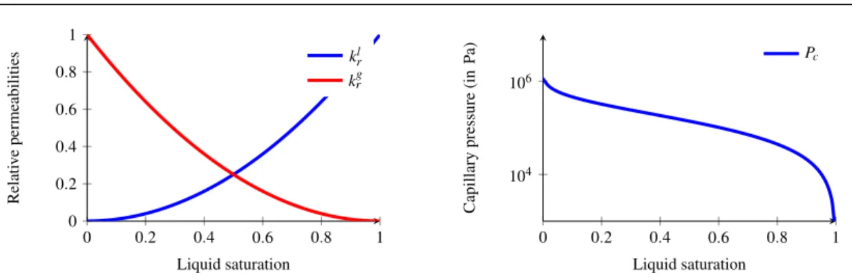
Fig. 6.2 Computational domain of the Darcy flow model coupled with the soil-atmosphere evaporation-outflow boundary condi-tion. krg(Sg) = 0 if Sg< Sgr, 1 if Sg> 1− Srl, √ 1− ¯Sl(1− ( ¯Sl)m1)2mif Sg r ≤ Sg≤ 1 − Slr, Pc(Sl) = Pr(( ¯Sl)− 1 m− 1)1n if 0 < ¯Sl≤ 1, with ¯ Sl= S l− Sl r 1− Sl r− S g r . 0 0.2 0.4 0.6 0.8 1 0 0.2 0.4 0.6 0.8 1 Liquid saturation Relati v e permeabilities kl r kgr 0.4 0.6 0.8 1 105 1010 Liquid saturation Capillary pressure (in P a) Pc
Fig. 6.3 Relative permeabilities of both phases kαr,α= g, l and capillary pressure Pcas functions of the liquid saturation Slof the Callovo Oxfordian clay.
The liquid and gas phases are a mixture of two components, the water denoted by w and the air de-noted by a. The gas molar density is defined by the perfect gas lawζg=RTPg, with R = 8.314 J. K−1. mol−1
and the liquid molar density is fixed toζl= 55555 mol. m−3. The phases viscosities are fixed toµg= 18.51· 10−6 Pa. s−1 andµl = 10−3 Pa. s−1. The gas fugacities are given by Daltons law for an ideal mixture of perfect gas fig= CgiPg, i = a, w. The fugacity of the air component in the liquid phase is given by Henry’s law fal = Cl
aHa(T ) with the temperature dependent Henry constant Ha(T ) = Ha1+
(Ha2− Ha1)TT−T1
2−T1 where Ha1= 6· 10
9 Pa, Ha
2= 1010 Pa, T1= 293 K and T2= 353 K. For the water
component in the liquid phase, the fugacity is taken from [38] fwl = ClwPsat(T ) exp ( −Psat(T )− Pl ζlRT ) ,
where Psat(T ) is the vapour pressure of the pure water given by the Rankine formula
Psat(T ) = 1.013· 105exp ( 13.7−5120 T ) .
The liquid molar enthalpy hland the gas molar enthalpy of the water component hg
ware taken from [38].
The gas molar enthalpy of the air component is given by hga(T ) = cgp,amaT where cgp,a= 1000 J. K−1. kg−1
is the specific heat capacity of pure air and ma= 29·10−3 kg. mol−1is the air molar mass. The gas molar
enthalpy is then defined by (2.1). The bulk rock thermal conductivity is fixed toλ= 10 W. m−1. K−1and the rock energy per unit volume is given by Er(T ) = 2· 106T in J. m−3with T in K.
The initial and top boundary conditions in the porous medium are defined by a liquid phase Sl= 1
with pure water Cwl = 1, Cal= 0, a temperature Tpm0 fixed either to 303 or 333 K and a hydrostatic pressure
with 38 atm at the top boundary. The lateral boundaries are considered thermally isolated (no Fourier flux) and impervious (no Darcy flux). The soil-atmosphere evaporation-outflow boundary condition at the interfaceΓ is set with no radiation nor precipitation recharge and the outflow liquid flux is vanishing during the overall simulation in the following test cases.
At the output boundaryΓout={l}×(0,hf f) of the free-flow domain, the pressure Pout= 105Pa is the
atmospheric pressure. The velocity at the input boundaryΓin={0}×(0,hf f) is defined by the uncoupled
turbulent velocity profile
u0(y) = ( u0(y) 0 ) ,
computed from the Prandtl algebraic turbulent model (see [29]), with an average velocity uin= 1 hff ∫ h ff 0 u0(y)dy = 0.5 m.s−1,
and such that u0(hf f) = u0(0) = 0. The temperature at the input boundaryΓinis fixed to Tin= 303 K and
the input molar fractions to Cin=
( Cw,in
1−Cw,in
)
with the relative humidityPoutCw,in Psat(Tin)
= 0.5.
An homogeneous Dirichlet boundary condition for the velocity and homogeneous Neumann boundary
conditions for the molar and energy transport are used at the boundary (0, l)× {0}. The turbulent
vis-cosityµtused in the free-flow domain to define the RANS stress tensor is given by the Prandtl algebraic
turbulent model as in [29] and computed once and for all from the uncoupled solution in the free-flow model. The turbulent diffusivity
Dt= Dg+µt−µ
g
ρgS
c
(6.1) is deduced using the gas Fickian diffusion Dg= 2· 10−5m2. s−1and the Schmidt number Sc= 1. The
turbulent thermal conductivity is similarly defined byλt=λg+ cgp,a(µt−µg) with the gas thermal
The simulation is run over the time interval [0,tf] with tf = 200 years, using an adaptive time step
starting with an initial time stepping of 1 s and a maximum time step of 10 years. The Cartesian mesh is uniform in the x direction with Nx= 100 edges and refined exponentially in the vertical y direction on
both sides of the interfaceΓ to account for the turbulent boundary layer and for the high gradient of the liquid pressure. More precisely, the porous medium mesh is defined by
Ne> 0, Ny> Ne, r > 1, ∆yr> 0,
such that hf f+∆yr(rNe− 1) < hpm. Numbering the y-edges (yi, yi+1), i = 1,··· ,Ny+ 1 from bottom to
top, we set yi= hf f+∆yr(ri−1− 1), 1≤ i ≤ Ne+ 1, yNe+1+ (i− Ne− 1) hpm− yNe+1 Ny− Ne , Ne+ 2≤ i ≤ Ny+ 1.
The numerical performances of the Darcy flow model coupled with the soil-atmosphere boundary con-dition are assessed on the following meshes
Ny= 30 with Ne= 10, r = 1.58, ∆yr= 1.43· 10−2,
Ny= 60 with Ne= 20, r = 1.28, ∆yr= 1.02· 10−2,
Ny= 90 with Ne= 30, r = 1.19, ∆yr= 8.40· 10−3.
The convective molar and energy transfer coefficients are computed from the following low frequency diagonal approximations of the Dirichlet to Neumann operators related to the uncoupled convection diffusion equations in the free-flow domain. Let us define the solutions c and T of the following linear convection diffusion equations by
ζg(P out, Tin)div ( cu0− Dt∇c ) = 0 onΩf f, c = 1 onΓ, c = 0 onΓin, ∇c · n = 0 onΓout, ∇c · n = 0 on (0,l) × {0}, (6.2) and div ( ζg(P out, Tin)∂ hgw ∂T (Pout, Tin)T u 0−λ t∇T ) = 0 onΩf f, T = 1 onΓ, T = 0 onΓin, ∇T · n = 0 onΓout, ∇T · n = 0 on (0,l) × {0}. (6.3) Then, we set Hm(x) =ζg(Pout, Tin)Dg∇c · nf f|Γ, HT(x) =λg∇T · nf f|Γ, (6.4)
with nf f the normal atΓ oriented outward to the free-flow domain.
Tables 6.1 and 6.2 compare, respectively for Tpm0 = 303 K and Tpm0 = 333 K and for the three meshes,
the numerical efficiency of the Newton-min non-linear solvers with their different improvements intro-duced in Section 4.1. Each table contains the number of successful time steps, the number of time step chops (i.e. the number of Newton-min convergence failures), the average number of Newton iterations per time step and the CPU time (in seconds on 2.9 GHz Intel Core i5 processor and 8Go RAM). It is shown that the basic Newton-min algorithm fails to converge in these test cases and that the use of the
Nx× Ny 100× 30 100× 60 100× 90
Basic Newton-min × × ×
Newton-min
157/0/3.71/147 157/1/3.97/552 × with projection
and non-linear phase
157/0/3.44/147 157/0/3.80/502 157/0/3.92/1012 appearance criterion
Newton-min
157/0/3.46/140 157/0/3.78/487 157/0/3.97/988 with projection and
thermodynamic equilibrium
Table 6.1 Number of successful time steps, of time step chops, average number of Newton iterations per successful time step and CPU time for the three Newton methods obtained with Ny= 30, 60, 90 and Tpm0 = 303 K.
Nx× Ny 100× 30 100× 60 100× 90
Basic Newton-min × × ×
Newton-min
157/0/3.52/142 157/0/3.90/497 180/2/4.09/1360 with projection
and non-linear phase
157/0/3.44/145 157/0/3.80/467 157/0/3.91/999 appearance criterion
Newton-min
157/0/3.39/138 157/0/3.73/523 157/0/3.90/972 with projection and
thermodynamic equilibrium
Table 6.2 Number of successful time steps, of time step chops, average number of Newton iterations per successful time step and CPU time for the three Newton methods obtained with Ny= 30, 60, 90 and Tpm0 = 333 K.
equilibrium phase molar fractions for the phase appearance criterion is necessary to obtain the
conver-gence for the finest mesh at Tpm0 = 303 K. On the other hand, imposing the thermodynamic equilibrium
at each Newton iterate improves only slightly the convergence.
The solutions of the liquid gas Darcy flow coupled either with the soil-atmosphere boundary
con-dition or with the full-dimensional gas free flow are compared using the finest mesh with Ny= 90.
Figures 6.4 and 6.5 exhibit, respectively for Tpm0 = 303 K and T0
pm= 333 K, the evolution in time of the
mean relative humidity, the mean temperature and the mean molar flow rate of the water component at the interfaceΓ for both models. The two stages, typical of drying processes, are clearly identified. The first stage corresponds to a high liquid evaporation rate combined with a relative humidity at the interface close to one. This stage is mainly governed by the free turbulent flow as long as the interface is water saturated. The second stage, triggered by the desaturation of the porous medium, corresponds to the drop of both the evaporation rate and the relative humidity reaching their stationary state say at time 200 years. The cooling effect of the liquid evaporation at the interface is also clearly observed in the temperature plot of Figure 6.4.
Figures 6.4 and 6.5 show that the soil-atmosphere boundary condition combined with the convective molar and energy transfer coefficients (6.4) provides a very good approximation of the coupled non-isothermal liquid gas Darcy and full-dimensional gas free flow model. The mismatch is larger for Tpm0 = 333 K than for Tpm0 = 303 K on the evaporation rate due to larger variations in time of the convective
molar and energy transfer coefficients not captured by Hmand HT. Nevertheless, the temperature and
relative humidity at the interface remains very well approximated in both cases.
7 1D and 2D geothermal test cases
In these simulations, the porous medium is homogeneous of porosityϕ(x) = 0.35 and of isotropic
per-meabilityΛΛΛ(x) = K× I with K = 1 D. The relative permeabilities are defined by kαr(Sα) = (Sα)2for
each phaseα∈ P. The capillary pressure function is given by the Corey law
Pc(Sg) = { −bln(1 − Sg) if 0≤ Sg≤ S 1 −bln(1 − S1) +1−Sb1(S g− S 1) if S1< Sg≤ 1