Optimization of the robot and positioner motion in a redundant fiber placement workcell

HAL Id: hal-01692417

https://hal.archives-ouvertes.fr/hal-01692417

HAL is a multi-disciplinary open access archive for the deposit and dissemination of sci-entific research documents, whether they are pub-lished or not. The documents may come from teaching and research institutions in France or abroad, or from public or private research centers.

L’archive ouverte pluridisciplinaire HAL, est destinée au dépôt et à la diffusion de documents scientifiques de niveau recherche, publiés ou non, émanant des établissements d’enseignement et de recherche français ou étrangers, des laboratoires publics ou privés.

Optimization of the robot and positioner motion in a

redundant fiber placement workcell

Jiuchun Gao, Anatol Pashkevich, Stéphane Caro

To cite this version:

Jiuchun Gao, Anatol Pashkevich, Stéphane Caro. Optimization of the robot and positioner motion in a redundant fiber placement workcell. Mechanism and Machine Theory, Elsevier, 2017, 114, pp.170 -189. �10.1016/j.mechmachtheory.2017.04.009�. �hal-01692417�

1

Optimization of the Robot and Positioner Motion in a Redundant Fiber

Placement Workcell

Jiuchun Gao

_{*, Anatol Pashkevich}

_{and Stéphane Caro}

a _{Ecole des Mines de Nantes, 4 rue Alfred-Kastler, Nantes 44307, France.}

b _{Institut de Recherches en Communications et Cybernétique de Nantes, UMR CNRS 6597, 1 rue de la Noë, 44321 Nantes, France.} c _{Centre National de la Recherche Scientifique (CNRS), France.}

* Corresponding author at: C022B, Ecole des Mines de Nantes, 4 rue Alfred-Kastler, Nantes 44307, France. Tel.: +33 6 58 48 14 16. E-mail address: jiuchun.gao@irccyn.ec-nantes.fr (J. Gao).

Abstract

The paper proposes a new methodology to optimize the robot and positioner motions in redundant robotic system for the fiber placement process. It allows user to find time-optimal smooth profiles for the joint variables while taking into account full capacities of the robotic system expressed by the maximum actuated joint velocities and accelerations. In contrast to the previous works, the proposed methodology possesses high computational efficiency and also takes into account the collision constraints. The developed technique is based on conversion of the original continuous problem into a discrete one, where all possible motions of the robot and the positioner are represented as a directed multi-layer graph and the desired time-optimal motions are generated using the dynamic programming that is applied sequentially for the rough and fine search spaces. To adjust the optimization results to the engineering requirements, the obtained trajectories are smoothed using the spline approximation. The advantages of the proposed methodology are confirmed by an application example that deals with a planar fiber placement robotic system.

Keywords

Redundant robotic system; Optimal motion planning; Graph-based representation; Dynamic programming; Robotized fiber placement

1. Introduction

Currently, composite materials are increasingly used in industry [1, 2]. Compared to traditional ones, they have good strength-to-weight ratio, durability, flexibility of shaping and corrosion resistance [3, 4]. Accordingly, they are extremely attractive for fabrication of large dimensional parts in aerospace, automotive and marine industries. The conventional way of manufacturing composite based components is labor intensive tape laying procedure. This manual process is quite slow and expensive, with low repeatability [3]. For efficient fabrication of composite parts, automated tape laying (ATL) is a more productive method. This is a specific technique which drives a technological tool laying a continuous composite tape onto molds automatically. However, ATL has a drawback that it is limited by the mold shapes. For a mold surface with high variation curvatures, tape wrinkling and overlap appear, and it decreases the mechanical performance of the composite dramatically [3, 5, 6]. For this reason, automated fiber placement (AFP) was proposed as an extension to ATL for fabricating composites with arbitrary surfaces [6, 7]. Instead of laying a single tape in ATL, heated fiber tows (12 to 32) are placed onto molds with desired orientations side-by-side and simultaneously. A pressure roller reinforces the placed fibers in situ [1, 3, 7]. Consequently, AFP becomes to the most widespread composite manufacturing technique because of the increasing demand for complex structural components [6].

The fiber placement process can be implemented by using either specifically designed machines or robotic systems, which are redundant in this application [3]. In the first case, general CNC machines equipped with specific placement head are used. They have no limitations on the workpiece size, but usually are quite expensive and require large work floor areas [7-9]. Compared to the process-dedicated machines, the robotic systems are relatively cheap and flexible allowing changing the product type easily [9]. In comparison to their size, they can provide a large working area. Industrial robotic systems are usually composed of a 6-axis serial robotic manipulator, a specific fiber placement end-effector and an actuated positioner

2 with one or two degrees of freedom [10, 11]. The workpiece is mounted on the positioner flange and changes its orientation with rotation of the positioner axis.

In robotic fiber placement process, manipulator motion planning is an important issue. The main difficulty here arises because of robotic system redundancy with respect to the manufacturing task. To generate the desired motion, it is required decomposing the given task into a robotic manipulator motion and a positioner motion. In literature, several works deal with this issue. A conventional way is based on redundancy resolution via the generalized inverse (pseudo inverse) of the kinematic Jacobian [12-15]. It gives a unique solution for the differential kinematic equations in the sense of least squares, which corresponds to the smallest Euclidean norm of the displacement vector in the joint space. However, this technique can hardly generate the time-optimal solution taking into account velocity and acceleration constraints of actuators, which are quite important in real-life industrial applications. Another approach of motion planning for redundant robotic system [16, 17] is based on the idea of “master-slave”, where the trajectories of the “master” manipulator are assigned firstly, and the corresponding conjugate trajectories of the “slave” are then determined. This method is rather simple and computationally efficient, but assigning the master trajectory is not trivial, especially for complex shape objects. Besides, here it is not possible to take into account the actuator constraints in an explicit way.

To generate the manipulator motion for complex shape workpiece taking into account constraints imposed by the actuators and avoiding collisions between the workcell components, several alternative methods have been developed that are based on direct optimization of an objective function describing the total travelling time, the trajectory smoothness, the quantity of manipulator motions, etc. One of such techniques [18, 19] is based on transformation of the original continuous time-optimal problem into a discrete one, where the robotic manipulator and the positioner joint spaces are discretized and the desired trajectory is represented as the shortest path on the corresponding graph. Then, the conventional discrete optimization techniques are applied to obtain the approximate time-optimal trajectory. A key issue here is related to assigning distances between the adjacent nodes of the graph, which are usually computed considering the velocity constraints only and omitting the acceleration constraints. The latter may lead to an optimal solution that corresponds to non-smooth manipulator trajectories, with essential oscillations in actuator velocities. Besides, conventional methods (Dijkstra algorithm, etc.) are rather time consuming for discretization steps acceptable in practice. Slightly different approach was proposed in [20-23] for the applications with constant Cartesian speed of the technological tool (robotic laser-cutting, spraying and arc-welding). In this case, the travelling time between the adjacent graph nodes is constant, so the required distances may be defined as the largest increments in the joint coordinates corresponding to the node-to-node movements. This allows to reduce oscillations in actuator velocities and to improve the trajectory smoothness, but the basic assumption of these techniques (constant tool speed) is not valid for the fiber placement. Nevertheless, some ideas from the above mentioned works, such as application of dynamic programming and elimination of nodes sequences violating the acceleration constraints, are useful for the problem studied in this paper.

For the fiber placement process, the problem of the manipulator motion planning was studied by Martinec [24] and Mlynek [25], who also assumed that the tool velocity is constant. Another work [26] focuses on the tool path optimization in Cartesian space while the optimal utilization of the robotic system redundancy was replaced by smoothing the end-effector trajectory. Obviously, this kinematic improvement does not allow using full capacities of the actuators, but it contributes to the trajectory smoothness in the configuration space and manufacturing efficiency by minimizing variations of the joint coordinates. To the best of authors’ knowledge, there are no techniques directly addressing the problem of the time-optimal motion planning for robotic fiber placement and it is still an open issue.

Besides optimization of the travelling time, improvement of the manipulator motion smoothness is another important issue in fiber placement applications. Smooth trajectories allow considerable reduction of vibrational phenomenon and mechanical wear of the robotic system. Known techniques in trajectory smoothing focused mainly on bounding the jerk value (defined as the derivative of the acceleration with respect to time) during the trajectory planning. For example, the maximum absolute value of the jerk is limited in [27-29], and the integral of the squared jerk along the trajectory is minimized in [27, 30-33]. Among the known works, it is also worth mentioning [30, 31] where an efficient minimum time-jerk trajectory planning algorithm was proposed for non-redundant robotic manipulators. However, these techniques cannot be directly applied to the motion planning for the redundant robotic system.

This paper focuses on optimization of manipulator motions in redundant systems taking into account two main objectives: (i) total travelling time, and (ii) trajectory smoothness. The proposed algorithm is an enhancement of our previous technique [34], it is based on the search space discretization and relevant combinatorial optimization search. In order to reduce computing time, the algorithm is composed of three stages: rough search, local optimization and smoothing. First, the original problem is presented as a combinatorial one after a rough discretization of the search space, and it is solved by using dynamic programming. An initial solution is generated quickly here. Then, the initial solution is sequentially improved by gradually

3 reducing the discretization step in its neighborhood and applying the same dynamic programming procedure. Further, the trajectory smoothing technique based on polynomial approximation of the positioner displacement profile is applied, and the corresponding robot displacement profiles are updated. This idea of sequential optimization allows us to obtain the desired manipulator motions in practically acceptable time.

The remainder of the paper is organized as follows. Section 2 presents the considered fiber placement robotic system. Section 3 deals with the system and task models and also presents the problem statement. Section 4 proposes the motion planning methodology, including the graph-based presentation of the search space and the developed optimization algorithm. Section 5 contains an application example that confirms the efficiency of the proposed methodology. In Section 6, some limitations and open issues are discussed. Section 7 concludes the contributions and defines future research directions.

2. Robotic fiber placement system

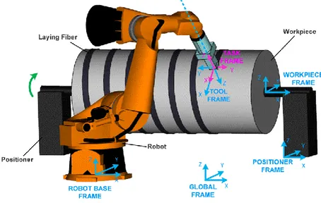
Typical robotic fiber placement system includes a 6-axis robotic manipulator and an actuated positioner with one or two degrees of freedom (see Fig. 1). The robotic manipulator is equipped with a specific technological tool ensuring fiber feeding, heating and compaction. The workpiece is mounted on the positioner allowing changing its orientation in order to improve accessibility of certain zones by the technological tool. In practice, a one-axis positioner is usually sufficient if the workpiece is not too large and its shape is simple. In the case of large dimension workpiece, the robotic manipulator can be located on a linear track increasing the robot workspace and its number of degrees of freedom. It is clear that this architecture including at least 7 actuators is redundant with respect to the considered technological task which requires 6 degrees of freedom only. This redundancy provides user with some flexibility because the same workpiece point can be reached with different configurations of the robotic manipulator and the positioner. On the other side, this essentially complicates the robotic system programming and poses a problem of using the redundancy in the best way.

Fig. 1 Typical robotic fiber placement system (6-axis robot and one-axis positioner)

To take into account particularities of the considered application, let us provide some details concerning the robot end-effector that is also called the fiber placement head [3, 6, 35]. This technological tool is usually composed of a material feeder, a fiber heater and a compaction roller, as shown in Fig. 2. The fiber tows are fed and guided towards the desired task locations with desired orientations. To heat fiber tows, a diode laser is used with active control during the placement process. The temperature of the material is controlled by adjusting the laser power, allowing maintaining the prescribed level and avoiding the material overheating. Finally, the heated fiber tows are consolidated in situ by compaction roller and cooled down.

In practice, the fiber placement head may have different designs in order to adapt it to the particular task. For workpieces with approximately cylindrical shape (liners of vessels, etc.) there are winding-oriented head designs. For workpieces with complicated 3D surfaces, there are laying-oriented designs of the head. It is worth mentioning that geometry of the fiber placement head imposes some extra constraints on the robotic manipulator configurations that must be taken into account in the motion planning procedure. In this paper, these constraints are evaluated at the stage of the search space generation, where some nodes of the original task graph are eliminated (they are treated as inadmissible ones because of collisions). In more details, this issue will be addressed in the section 3.3.

4

Fig. 2 Robot end-effector for automated fiber placement (AFPT GmbH)

In current industrial practice, programming of robotic system essentially relies on a set of software modules allowing user to prepare the program in off-line mode and avoid time consuming manual teaching. To take into account the system redundancy, we propose the following robot programming procedure presented in Fig. 3. It is assumed that the workpiece model was already created in a CAD system. It is used as the input of the dedicated CAM system that provides the fiber placement path generation in Cartesian space and its discretization (with respect to the workpiece frame). Further, the obtained set of path points and related frames (task model) is entered in the graph generator, which transforms it into a so-called “task graph” that describes all possible motions of the robot and the positioner joints ensuring the desired fiber placement path on the workpiece. It should be mention that this graph takes into account the robotic system redundancy because each graph node represents certain configurations of robot and positioner but each task location corresponds to a number of nodes (graph layer). Using this graph, the next software module provides generation of optimal motions for the robot and positioner. These motions are presented as the “best” path on the graph connecting two boundary layers corresponding to the initial and final locations of the fiber placement task. Finally, the obtained robot and positioner motions are converted into the robotic system program by the post processor. It worth mentioning that this idea of graph-based representation of possible robot/positioner motions was previously successfully used for robotic laser cutting applications [20-22] but these results cannot applied directly here for the considered technology. The open questions are related to formalization of the “best” path notion and development of dedicated algorithm for the “best” path search. These issues are addressed in this paper.

Fig. 3 Preparation of manufacturing process for robot-based fiber placement

3. System model and task formalization

The key problem addressed in this paper is to find optimal motions of robot and positioner ensuring desired trajectory of the technological tool with respect to the workpiece and satisfying some constraints imposed by the system kinematics and the fiber placement technology. To present this problem in a formal way, let us consider in details the system geometry and define optimality criteria for the robot and positioner motions.

3.1 Fiber placement task model

Let us assume that desired fiber placement path is presented as a 3D-augmented line in relevant CAD system and discretized in n segments. This presentation allows obtaining both the Cartesian coordinates of the path points T

i i i i(x ,y,z)

5 the unit vectors T

zi yi xi i(a ,a ,a )

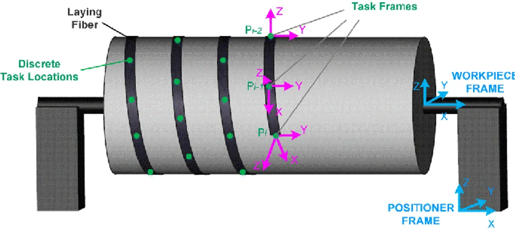
a defining the workpiece surface normal directions. To get corresponding end-effector locations required for the robot programming, let us introduce a set of coordinate frames associated with each path point (see Fig. 4). These frames are defined as follows: (i) the frame origin is located at the path point p ; (ii) the X-axis shows the i

motion direction and coincides with the path tangent; (iii) the Z-axis points the surface normal direction and coincides with the vectora ; (iv) the Y-axis is perpendicular to the axes X and Z to complete a right-handed frame. The main difficulty here is i related to computing of the X and Y directions described by the unit vectors T

zi yi xi i(n ,n ,n ) n and T zi yi xi i(s ,s ,s ) s respectively,

which usually cannot be extracted directly from the CAD model. To find these two vectors, the following procedure can be applied. First, the X-direction is estimated approximately using the path incrementpi (pi1pi). Then, the Y-direction is computed via the vector product si aipiand normalized as si:si/ si . Finally, the vector of the X-direction is computed

straightforwardly using the formula nisiai.

Using the above frames, the fiber placement task can be presented as a set of locations that should be visited sequentially by the robot end-effector in minimum time. Assuming that each location is described by a 44homogenous transformation matrix, the considered task is formalized as follows

) ( ) ( ) 2 ( ) 1 ( _{... ...} n task w i task w task w task w_{T  T  T   T (1)} where 1 ... , 2 , 1 , 0 ; 1 0 0 0 ₄₄ ) ( _{ }         n i i i i i i task w_T n s a p

and all vectors are expressed with respect to the workpiece base frame (see superscript “w”). Equivalent presentation of the considered task relies on 61vectors that include three Cartesian coordinates and three Euler angles that can be easily computed from the orientation matrices (ni,si,ai)33[36].

Fig. 4 Discretization of the fiber placement path and definition of the task frames

3.2 Robotic fiber placement system model

As shown in Fig .1, the considered robotic fiber placement system includes two principle mechanisms: an industrial robot (a technological tool manipulator) and a positioner (a workpiece manipulator). It is assumed that their kinematics is known and spatial locations of the output frames depend on the vectors of actuated joint coordinatesq and R qPrespectively. Let us derive

the kinematic model of the whole system that includes the closed loop created by the robot, workpiece and positioner.

The robot kinematic model describes the end-effector frame location (position and orientation) with respect to the robot base as a function of the actuated joint coordinates. For the serial architecture, the robot model can be presented as a product of the 44homogenous transformation matrices

6     6 1 i 1 _{( )} ) ( Ri R_i i R R q g q T (2)

depending on corresponding joint angles [36]. This model is also often referred to as the direct kinematics of the robot. Particular expressions for the matrices Ri

i1_{T can be obtained using the Denavit-Hartenberg (DH) technique [37], where they}

are presented as a composition of elementary rotations and translations ( ) ( 1) ( 1) ( Ri) ( )

1 i Z Z i X i X Ri Ri i _{T q R D a R q D d}    _

depending on both the joint variables q and the parameters Ri ai,di,idescribing the links/joints geometry.

In practice, it is also often used the inverse kinematic model 1(.)

R

g that allows user to compute the vector of the actuated joint variables q corresponding to the desired end-effector location described by a given homogeneous R 44 matrix T .

Compared to the direct kinematics, the inverse one is not trivial since the solution is usually not unique and cannot be expressed in a closed form. For this reason, special types of manipulator architecture are used to satisfy the Pieper condition [38] that ensures the closed-form solution. Otherwise, there are also some numerical techniques to deal with this problem [39, 40]. In our study, the serial robot with last three intersecting axes is employed, which corresponds to the majority of industrial applications. It should be also stressed that in order to obtain a unique solution, the inverse kinematic function augments also include the so-called configuration index  that determines the posture of the manipulator shoulder, elbow and wrist. For this reason, in the following sections the inverse kinematic function will be referred to as 1(_T,_)

R

g .

The positioner kinematic model describes the positioner mounting flange location with respect to its base as a function of the actuated coordinate vector q . Similarly to the above case, it can be also presented as a product of the matrices P

    P N i Pi Pi i P P q g 1 1 _{( )} ) (q T (3) that may be derived using the Denavit-Hartenberg technique (usuallyNP1,2, since typical positioner has one or two degrees of freedom). Because of lacking degrees of freedom, the inverse kinematics for the positioner cannot be solved in strict way [41]. But it is not important for technique developed in this paper that employs the positioner direct kinematic model only.

To obtain the kinematic model of the whole system, let us assume that for technological reasons the end-effector frame and the task frame must be aligned in such way that: (i) the origins of these two frames coincide; (ii) their X-axes are directed similarly; (iii) their Z-axes are opposite. This assumption corresponds to the following homogeneous transformation matrix defining a relation between the end-effector and task frames

               1 0 0 0 0 1 0 0 0 0 1 0 0 0 0 1 task tool_T (4)

It allows us to express global locations of all task frames in two ways, using either the robot or positioner kinematic models. In the first case, the matrices 0 (i)

task

T describing the task frames are presented as follows

n i g task tool i R R Rbase i task ( ) ; 1,2,... ) ( 0 ) ( 0_{T  T  q  T  (5)} where TRbase

0 _{defines the robot base location relative to the global system that is denoted by the superscript “0” (see Fig. 1). In the}

second case, similar matrices are expressed as

n i g i task w i P P Pbase i task ( ) ; 1,2,... ) ( ) ( 0 ) ( 0_{T T  q  T  (6)} where TPbase

0 _{defines the positioner base location relative to the global system and the superscript “w” denotes the workpiece}

coordinate system.

7 n i g g i task w i P P Pbase task tool i R R Rbase ( ) ( ) ; 1,2,... ) ( ) ( 0 ) ( 0_{T  q  T T  q  T  (7)}

describing relations between the actuated coordinates of the robot and the positioner, which ensure implementation of the given technological task. It is clear that because of the system redundancy, the above equations do not allow to obtain a unique solution for q and R q corresponding to each task point. On the other hand, it provides us with some space for the P

robot/positioner motion optimization where the above equations are treated as the hard constraints. 3.3 Problem of robot/positioner motions planning

To utilize the redundancy in the best way, it is reasonable to partition the desired motion between the robotic manipulator and the positioner in such a way that the technological tool executes the given task as fast as possible and the robot and positioner movements are smooth enough. These objectives are obviously constrained by the actuator capacities that can be expressed as the maximum allowable joint velocities and accelerations.

To present this problem in a more formal way, let us introduce the functions qR(t)and qP(t)that describe the robot and

positioner motions on the time interval t[ T0, ]. In addition, let us define the time instances {t1,t2,...tn} corresponding to the cases where the robot end-effector visits the task frames defined by Eq. (1), where t10, tnT. Using this notation, the

problem can be presented as minimization of the total travelling time

) ( ), ( min_{t t} P R T_{q q} (8)

over the set of continuous functions qR(t)and qP(t) subject to the equality constraints imposed by the prescribed task

n i t g t g i task w i P P Pbase task tool i R R Rbase ( ( )) ( ( )) ; 1,2,... ) ( 0 0_{T  q  T  T  q  T  (9)}

and the inequality constraints describing the capacities of the robot/positioner actuators max min

₍

₎

q

t

q

q





q



q

(

t

)



q

₍

₎

q

t

q

q











q





q



(

t

)



q



₍

₎

q

t

q

q











q





q



(

t

)



q



where j is the index for the robot and positioner joint variables: j1,2,...6 for the robot and j1,2 or j1for the positioner.

Besides, the collision constraints that are extremely important for the considered technological application must be taken into account. They are defined as follows:

] , 0 [ ; 0 )) ( ,) ( ( t t t T cols q_P q_P    (11)

where the binary function cols(.) verifies the intersections between the robotic system components (manipulator and positioner links, workpiece, fixture, etc.). It should be mentioned that the fiber placement head geometry may cause very restrictive collision constraints (see Fig. 2). To take into account this issue, additional verifications of intersection between the workpiece and the robot end-effector are required. In practice, relevant collision detection functions may be implemented using standard routines of commercially valuable industrial robotic CAD packages.

For this optimization problem, which aims at finding continuous functions qR(t)and qP(t)describing the robot manipulator

and positioner motions, there is no known technique that can be straightforwardly applied to. The main difficulty here is related to the equality constraints that are written for the unknown time instants t1,t2,...tn. Besides, this problem is highly

nonlinear and includes redundant variables. It should be mentioned that for the non-redundant case without the collision constraints the problem was solved by Bobrow et al. [42]. Another technique proposed in [18, 19] deals with the redundant case, but the collision constraints are verified at the post-optimization stage. For these reasons, this paper proposes a discrete optimization based methodology that is able to take into account simultaneously the system redundancy, the actuator capacities and the collision constraints.

8 4 Motion Planning Methodology

In order to solve the considered problem, a combinatorial optimization based methodology is proposed in this section. It includes three principal steps: a) search space discretization; b) path planning; c) motion smoothing. Using this methodology, the considered Cartesian task is represented as a directed multi-layer graph, which allows us easily applying the dynamic programming. To improve the computational efficiency, the optimization is performed in two stages combining “global rough search” and “iterative local fine search”. Also, several strategies are proposed to adjust the trajectory to the requirements of the robot controller.

4.1 Search Space Discretization

For the considered robotic system, which includes a 6-axis robot and a one/two-axis positioner, there are exactly one or two redundant variables with respect to the given task (1) that is defined as a sequence of the robot end-effector locations in 6-dimensional space. First, let us present the one-axis positioner case and generalize it for the two-axis positioner further.

It is clear that for the one-axis positioner any of the manipulator joint variables included in the vector q can be treated as a R

redundant one, but it is more convenient to consider the positioner joint angle qP as the redundant variable. This allows us,

after solving the positioner direct kinematics for any given qP , to apply straightforwardly the manipulator inverse kinematic

function 1(_T,_)

R

g and find corresponding vectors q for the robot (which are not unique because of multiplicity of possible R

configurations defined by the parameter , see Section 3.2). This approach permits to take into account explicitly the equality constraints presented by Eq. (7) and substantially reduce the search space dimension.

To present the problem in a discrete way, let us sample the allowable domain of the redundant variable [ min, max]

P P P q q q  with the stepqP m k k q q q P P k P ; 0,1,... min ) ( _{    (12)} where m(qP qP )/qP min

max _{.Then, applying sequentially the positioner direct kinematics and the manipulator inverse}

kinematics in accordance with Eq. (9), one can get a set of possible configuration states for the robotic system. For the unique mapping from the task space to joint space, let us also take into account the configuration index  that corresponds to the manipulator posture, and specifies the shoulder, elbow and wrist configurations. Then, the manipulator configuration corresponding to the given (k)

P

q can be obtained as follows:





task_{T denote the inverse of} Rbase T 0 _and task tool_{T respectively;} i

t specifies the unknown time instant

corresponding to the task location (i)

task

w_{T ; the functions (.)} P

g and 1(.)

R

g denote the positioner direct kinematics and the manipulator inverse kinematics. Therefore, for each task location we can generate a number of configuration states, i.e.,

i k i k task i task w_T() _L( ,)_{;  , , where} (,) ₍ ()_{( ,)} ( )_{( ))} i k P i k R i k task q t q t

L  will be further referred to as the task location cell. Taking into account that the task locations are strictly ordered in time, the original sequence of (i)

task

w_{T described by Eq. (1)}

may be converted into the directed graph presented in Fig. 5. It should be noted that some of the configurations generated using Eq. (13) should be excluded from the graph because of the collision constraints (11) violation or exceeding of the actuator joint limits (10a). Besides, from an engineering point of view, it is prudent to avoid some configurations that are very close to the manipulator singular postures. These cases correspond to the “inadmissible nodes” in Fig. 5, which are not connected to any of the neighbors. It is clear that due to time-irreversibility, the allowable connections between the graph nodes are limited to the subsequent configuration states (,)_ (k,i1)

task i k

task L

L and the edge weights correspond to the minimum travelling time that are restricted by the maximum actuator velocities expressed by the constraints (10b).

9

Fig. 5 Graph-based presentation of the discrete search space (for one-axis positioner)

An outline of the graph generation Algorithm 1 is presented below (the algorithm is written in generic mathematical language, but it has been tested using the Matlab and C++ environment, see Section 5). The algorithm input is a sequence of

4

4 location matrices Task(i)corresponding to (i)

task

w_{T . The upper and lower limits of the redundant variable are defined as}

max

P

q and min

P

q respectively. The discretization density m determines the number of the discrete values of the redundant variable. The algorithm operates with the positioner direct kinematic function gP(.)and the robot inverse kinematic function to transform the task locations Task(i) into the joint space. The procedure is composed of two basic steps. The first step discretizes the redundant variable in the interval [ min, max]

P

P q

q by implementing formula (12), and mn matrix } ... , 2 , 1 ; ... , 2 , 1 ) (

{qP k,i i nk m is obtained. In the second step, the functions gP(.)and (.)

1 

R

g are applied sequentially, and the robot configuration states corresponding to {qP(k,i)i;k} are computed. It should be mentioned that the configuration index

 here is treated as a constant input parameter, while in practice the step (2) should be re-executed for each possible . The sub-step (2a) checks the solution of the robot inverse kinematics for each {qR(k,i)i;k} and applies the collision test function for each configuration state {qP(k,i),qR(k,i)i;k} . Finally, the task graph is generated with nodes

)) ( ), , ( ( ) (k,i q ki R k,i

L  P q . If a collision is detected or the function (.)

1 

R

g returns the “null” denoting that the robot inverse kinematics is not solvable (because of the joint limits violation, etc.), the “null” value is assigned to the current node (it is marked as “inadmissible” one on Fig. 5).

10 Using this presentation of the search space, the considered problem can be transformed to the searching of the shortest path on the directed graph shown in Fig. 5, where each column corresponds to the same task location (i)

task

w_{T and each row}

represents the same value of the positioner joint coordinate (k) P

q . In accordance with the physical sense, the initial and final path nodes must belong to the sets { , 1}

) 1 (k1, k task  L and { ( ), } n ,n k task k n 

L respectively. In the frame of this notation, the desired solution can be represented as the sequence of the nodes

} ...{ } { } { (11) (22) (k,n) task , k task , k task n L L L   (14)

corresponding to the robot and positioner configuration states ( ()( ,) ( )( ))

i k P i k R t q t q .

In accordance with the actuator constraints (10b), the distance between subsequent graph nodes can be evaluated as the displacement time for the slowest joint





where j0 corresponds to the positioner joint variable q and P j1,2,...6 correspond to the joint coordinates of the robot.

The latter allows us to present the objective function (total travelling time) as the sum of the edge weights

      1 1 ) 1 ( ) ( _{, )} ( 1 n i ,i k task ,i k task i i dist T L L (16)

that depends on the indices k1,k2,...kn. It should be noted that the applied method of edge weights computing automatically

takes into account the velocity constraints (10b), but the acceleration constraints must be examined for each considered path. It can be done by applying a formula

Algorithm 1: Search space generation G(.)

Input: Task location matrices {Task(i)i1,2,...n}

Upper limits of redundant variable {_qmax(_i)_i 1,2,..._n}

P 

Lower limits of redundant variable {_qmin(_i)_i 1,2,..._n}

P 

Discretization density m

Robot configuration index 

Output: Matrix of locations {L(k,i)k1,2,...m;i1,2,...n}

Notations: q_P, q_R - positioner and robot joint coordinates

T_P,T_R - Matrices of robot tool and positioner flange in local frames

Invoked functions: Robot inverse kinematics 1(.)

R

g in local frame Positioner direct kinematics gP(.)in local frame

Transformation from robot base to positioner base Trans(.) Collision test function cols(.)

(1)Redundant variable discretization

For i1 to n do _q(_i):_(_qmax(_i)_qmin(_i))/(_m1); P P P For k1 to m do _q(_k,_i): _qmin(_i) (_k 1) _q (_i); P P P    

(2)Location matrix creation For i1 to n do For k1 to mdo (a)TP:gP(qP(k,i))Task(i) ; TR:Trans(TP ); ( , ): 1( ,_); R R R ki g T   q (b) If (qR(k,i)null) (cols(qP(k,i),qR(k,i))1) L(k,i):null; else L(k,i):{qP(k,i),qR(k,i)};

11 max 1 1 ) ( 1 , ) ( 1 ) ( ) ( 1 , ) ( ) ( ) ( 2 1 1 j i i i i k i j k i k k i j i q t q t t t t q t i  i  i  i        qj,i  qj,i    (17)

which is based on the second order approximation of the corresponding functions qR(t)and qP(t) in the time domain, and

where ( ( ), ( 1)) 1 1     k ,i task ,i k task i i i dist t L L and   (( ), (k1,i1)) task ,i k task i i i dist t L L .

It is clear that for the one-axis positioner any of the manipulator joint variables included in the vector q can be treated as a R

redundant one, but it is more convenient to consider the positioner joint angle q as the redundant variable. This allows us, P

after solving the positioner direct kinematics for any given q , to apply straightforwardly the manipulator inverse kinematic P

function 1(_T,_)

R

g and find corresponding vectors q for the robot (which are not unique because of multiplicity of possible R

configurations defined by the parameter , see Section 3.2). This approach permits to take into account explicitly the equality constraints presented by Eq. (7) and substantially reduce the search space dimension.

For the case of a two-axis positioner, where the degree of redundancy is equal to two, the above presented methodology can be generalizedin the following way. Similarly to the previous case, letus treat the robot joint angles q as non-redundant R

variables and the positioner joint angles [ , max]

1 min 1 1 P P P q q q  and [ , max] 2 min 2 2 P P P q q

q  as the redundant ones which are sampled with the stepqP1and qP2respectively

1 1 1 1 min 1 ) ( 11 q q k ; k 0,1,...m qk _{P P} P     2 2 2 2 min 2 ) ( 2 ; 0,1,... 2 q q k k m q P P k P     (18) where 1 min 1 max 1 1 (qP qP )/ qP m    and 2 min 2 max 2 2 (qP qP )/ qP

m    . Then, applying sequentially the positioner direct kinematic and robot inverse kinematic transformations in accordance with (9), a set of possible configuration states for each task location can be found. This allows us to obtain a 3D directed graph where each Cartesian task location is presented by a set of nodes located on the plane (see Fig. 6) in contrast to the one-axis positioner case where each task location corresponds to a column (see Fig. 5). Using this graph, the desired robot/positioner motion can be presented as a shortest path that sequentially connects the nodes belonging to the above mentioned planes (exactly one node for each plane). It is clear that the same methodology can be applied for the robot with extra degrees of freedom, mounted on a linear track for example. In the latter case the set of redundant variables includes both the positioner actuated coordinates and the additional coordinates of the robot. This allows us to utilize analytical expressions for the robot inverse kinematic transformations.

12 4.2 Motion Planning Algorithm

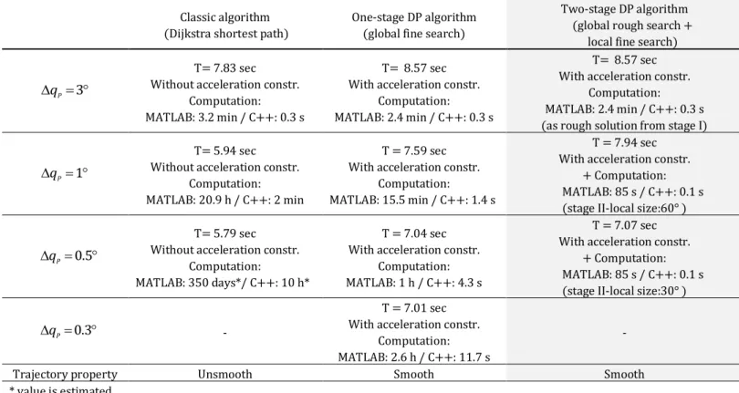
After generation of the discrete search space, the original optimization problem (8)-(10) can be converted to a combinatorial one, which is aimed at searching of the shortest path connecting the subsets of the nodes corresponding to the given task locations. For computational convenience, these subsets are grouped in columns for the one-axis positioner (see Fig. 5) and in planes for the two-axis positioner (see Fig. 6). A conventional way to solve this discrete optimization problem is to use the classical shortest path search on the directed graph (e.g. Dijkstra, Belford, etc.) created by adding two virtual nodes to the graph-based search space at the beginning and the end [18-20]. This path should visit exactly one node in the candidates for each task location. However, as follows from the dedicated study, the classical techniques are extremely time-consuming, and they can be hardly accepted for real-life industrial applications. For example, it takes over 20 hours using Matlab (and about 2minutes in C++) to find desired solution even in the relatively simple case that deals with a two-axis robot and one-axis positioner, where the search space was built for 100 task points and the discretization step 1° (Win7SP1 with Intel® _i5 @2.67 GHz 2.67 GHz). Besides, classical methods are not able to take into account the acceleration constraints expressed by inequalities (10c), which are important here because of technological requirements. For these reasons, a special problem-oriented algorithm is proposed below, which takes into account particularities of the graph describing the search space.

4.2.1 Motion generation using dynamic programming

To present the proposed algorithm for the general case, let us assume that the graph nodes corresponding to the same task points { (i)}

task

w_{T are organized as one-dimensional arrays {} (k,i)_{;i const}}

task 

L that are indexed by the superscript k0,1,...n. Such presentation is straightforward for the one-axis positioner, and it can be easily obtained by simple node renumbering in the case of the two-axis positioner. This allows us to describe the algorithm in similar way independent on the number of the redundant variables.

The developed algorithm is based on the dynamic programming principle, which breaks down the full-size problem into a set of sub-problems of smaller sizes [43], aiming at finding the shortest path from the initial node set to the current node set. To present the basic idea, let us denote dk,i as the length of the shortest path connecting one of the initial nodes { , 1}

) 1 (k1, k

task 

L to

the current node { ( i,k )}

task



L . Then, taking into account the additivity of the objective (16), the shortest path for the nodes corresponding to the next task point { (k,i1), _k}

task 



L can be found by combining the optimal solutions for the previous column }

, { (k,i) _k

task  



L and the distances between the nodes with the indices i and i1.The latter corresponds to the formula

; } ) , ( { (, 1) ( ) , 1 , ,i k task i k task i k k i k d dist d      min  L L (19)

that is applied sequentially starting from the second task point, i.e. i1,2,...n1. Finally, after selection of the minimum length dk,i1 corresponding to the final task point and applying the backtracking, one can get the desired optimal path.

Therefore, the desired solution for nsets { (11)} { (22)} ...{ (k,n)} task , k task , k task n L L

L   is obtained by increasing sequentially the i-index, computing dk,i1, and finding the minimum value among dkn,n. The desired path is described by the recorded indices

} ,... ,

{k1 k2 kn .

An outline of the proposed algorithm is presented below (see Algorithm 2). The input is the matrix of the locations } ... , 2 , 1 ; ... , 2 , 1 ) , (

{Lk i i n k m , which contains information on the configuration states satisfying the equality constraint (9) and the collision constraint (11). The algorithm operates with two tablesD( ik, ),P( ik, ) that include the minimum distances for the sub-problem of lower size (for the path 1i) and the pointers to the previous locations respectively. The procedure is composed of four basic steps. The step (1) initializes the distance and pointer matrices by defining their first columns. In step (2), the recursive formula (19) is implemented. The computing starts from the second column and tries all possible connections between the nodes in the current column {L(k,i),k} and the previous one {L(j,i1),j}. For the admissible configuration states, the acceleration constraints are examined using the expression (17) for each candidate path connecting the nodes with the indices i, i1and i2. In the algorithm, the acceleration constraint test is included in sub-step (2a) where accl()0indicates that the current path satisfies this constraint, and it begins from the third column. It should be mentioned that the function accl requires three inputs (.) L( ,i* ), L(*,i1), L(*,i2), according to the expression (17), and the locationL(*,i2) is determined using the pointerP( j,i-1) to the previous location in the current path. Then, sub-step (2b) finds the minimum path from the current node L( ik, )to the first column {L(j,1),j}and records the reference to

} ,) 1 , (

{L ji j into the pointer matrix. In steps (3) and (4), the optimal solution is finally obtained and corresponding path is extracted by means of the backtracking.

13 It is worth mentioning that the above presented algorithm is written in generic mathematical language, but it has been tested using the Matlab and C++ environment (see Section 5). As follows from a dedicated study, the proposed algorithm is rather efficient and suits industrial requirements in certain degree. In particular, it takes about 10 minutes using Matlab (and about 1 second using C++) to find the optimal solution for the above mentioned example (two-axis robot and one-axis positioner, 100 task locations, discretization step 1°). It should be stressed that in contrast to the conventional techniques, this algorithm can generate smooth trajectories by taking into account the acceleration constraints which are expressed by inequalities (10c). Nevertheless, since the inequalities (17) are checked for each candidate path during searching, the computation time may be still too high for real-life fiber placement applications where 6-axis robots are usually used and the number of the task points is essentially larger. This motivates us to improve the developed algorithm further.

4.2.2 Enhancement of the motion generation algorithm

To reduce the computing time, let us apply the following heuristic technique: solve the problem applying twice the same optimization routine (Algorithm 2) in different search spaces. It is reasonable to start with a rather big discretization step

P

q

 (stage I), and further improve the initial solution in its neighborhood using relatively small qP (stage II). In this

technique, in spite of the repetition of the basic optimization routine, both stages operate with the search space of smaller size compared to the straightforward optimization presented above, which allows us essentially decreasing the amount of the computations. The details of this technique are presented in Fig. 7.

Algorithm 2: DP-based Path planning DP(.)

Input: Matrix of locations {L(k,i) i1,2,...n;k1,2,...m}

Output: Minimum path length D min

Optimal path indices {_k0(_i)_i1,2,..._n}

Notations: D( ik, ), P( ik, )- distance and pointer mn matrices

Invoked functions: Distance between nodes dist(L(k1,i1),L(k2,i2))

Acceleration test for nodes accl





(1) Set D(k,1):0; P(k,1):null,k1,2,...m

(2) For i2 to n do For k1 to mdo

(a) For j1 to m do

If



 



If

 









else r( j):inf ; (b) Set D(k,i): ({r(j) j 1,2,...m}) j  min ; P(k,i): ({r(j) j 1,2,...m}) j  argmin ;

(3) Set Dmin:min_k ({D(k,n)k1,2,...m}); _k0(_n): ({_r(_j) _j 1,2,..._m})

k 

argmin ;

(4) For in to 2

14

Fig. 7 Two-stage technique for robot and positioner motion generation

The stage I, named here as the global rough search, is based on the full-range discretization of the redundant variable with relatively big increment step (compared to that in the fine search algorithm presented before). By applying the dynamic programming principle expressed by (19), an initial solution can be obtained quite rapidly (it takes about one minute using Matlab for the above presented example that deals with the two-axis robot and one-axis positioner, 100 task locations). It should be mentioned that the motion obtained at this stage may be not satisfactory from the engineering point of view since the discretization step is large. So, it is reasonable to optimize the obtained solution further.

At the stage II (named as the iterative local fine search), a secondary discretization with smaller step is applied in the neighborhood of the initial solution obtained at the stage I. The neighborhood size is defined by the user (Fig. 8). It is clear that this local discretization produces the search space of relatively small size (compared to straightforward approach, see Algorithm 1) allowing us quickly generate an optimal solution that is obviously better than the initial one. For instance, for the above mentioned example, it takes about two minutes using Matlab in total (stages I and II) while the one-stage technique (see section 4.2.1) requires more than 10 minutes to obtain a similar result. It should be mentioned that the stage II can be repeated several times, sequentially reducing the discretization step.

Fig. 8 Search space evolution for the two-stage algorithm

An outline of the two-stage algorithm is presented below (see Algorithm 3). The input includes the task location matrices } ... , 2 , 1 ) (

{Taski i n , the boundary limits of the redundant variable max

P

q and min

P

q , the neighborhood size RgPfor the stage II, and

the discretization densities m and mfor both stages. It outputs the minimum path length Dmin and optimal path indices } ... , 2 , 1 ) (

{_k0 _{i i n . At the first stage, the mn task graph {L(k,i)k1,2,...m;i1,2,...n} is generated using the full-range} discretization with the density m (step Ia). The initial solution{k0(i) i1,2,...n} is obtained by applying the path planning

15 new graph{L(k,i)k1,2,...m;i1,2,...n} of the size mn is generated in the neighborhood of the initial solution (step IIb). After applying again the planning function DP (step IIc), the optimal solution of the length (.) D_min and corresponding path indices {_k0(_i)} _{are obtained. The optimal trajectory is extracted at the step (IId).}

An alternative way to speed up the motion generation algorithm is to replace the stage II by simply smoothing the curve )

(t

qP corresponding to the redundant variable without changing the time instants obtained from the stage I (if it is acceptable

from technological point of view). This can be achieved by applying the polynomial approximation to the function defined by the nodes{qP(i),t(i)i1,2,...n}. From our experience, the 5th order polynomials are quite satisfactory for this procedure, which generates modified values of the redundant variable {qP(i)i1,2,...n} ensuring better profile of the curve qP(t). Then,

in order to guarantee that the task locations are exactly visited by the end-effector, the robot joint coordinates should be also regenerated using the new values of the redundant variable {qP(i)i1,2,...n} and sequentially reapplying the positioner direct kinematic and robot inverse kinematic transformations (see section 4.1). It is worth mentioning that the smoothing-based technique is very time efficient because it excludes the optimization at the stage II. However, in most cases studied by the authors the two-stage technique including the local optimization (see Fig. 6) provided better results.

4.3 Optimal Motion Implementation in Robotic System

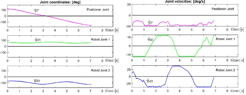
The above presented algorithm allows user to find the optimal robot and positioner motion, which are presented as the sequence of the nodes defining the joint coordinates {qRi,qPi i1,2,...n} corresponding to the time instants {ti i1,2,...n}. It

should be stressed that the time instants obtained from the motion planner are distributed irregularly in the interval [0,t . n] For this reason, while implementing this motion in industrial environment, it is necessary to take into account specific

Algorithm 3: Two-stage path planning

Input: Task location matrices {Task(i)i1,2,...n}

Upper limit of redundant variable max

P

q

Lower limit of redundant variable min

P

q

Neighborhood size RgP

Primary discretization density m Secondary discretization density m

Output: Minimum path length Dmin

Optimal path indices {_k0(_i)_i1,2,..._n}

Notations: { k,iL( )} - mn matrix of locations for the first stage

{L(k,i)} - mn matrix of locations for the second stage

Invoked functions: Graph generation (.)G ; (algorithm 1)

Path planning DP(.); (algorithm 2)

Stage I:

(a) Generate an initial graph using rough discretization in full domain of qP

Set {_L(_k,i) _i 1,2,..._n;_k 1,2,..._m}: _G





P P     (b) Apply algorithm DP(.) Set {{ () 1,2,... }; min}:





(c) Extract initial trajectory

For i1 to n do _InitTraj(_i)_L(_k0(_i),_i);

Stage II:

(a) Redefine the discretization domain

For i1 to n do

min() max{( ( .) ), min};

P P P

P i InitTraj i q Rg q

q  

max() min{( ( .) ), max};

P P P

P i InitTraj i q Rg q

q  

(b) Generate local graph using fine discretization in local domain of qP

Set {_L(_k,i) _k 1,2,..._m;_i 1,2,..._n} _G





P P            

(c) Apply algorithm DP(.) again

Set {{ () 1,2,... }; min}:





0 _{i i n D DP L k,i i nk m}

k        

(d) Extract optimal trajectory

For i1 to n do _OptTraj(_i)_L(_k0(_i),_i);