Title of Publication Edited by
TMS (The Minerals, Metals & Materials Society), Year
CHARACTERISATION OF THERMOPHYSICAL PROPERTIES
OF SEMI-SOLID STEELS FOR THIXOFORMING
J. Lecomte-Beckers1, A. Rassili2, M. Carton1, M. Robelet3 1
MMS (IMGC, Bât. B52), University of Liège, Sart Tilman, 4000 Liège, Belgium 2
Institut montefiore, University of Liège, Sart Tilman, 4000 Liège, Belgium 3
ASCOMETAL CREAS, BP 750042, 57301 Hagondange Cedex, France Keywords: Thixoforming, Thermophysical properties, Liquid fraction
Abstract
Major challenge for semi-solid processing includes broadening the range of alloys that can be successfully thixoformed and developing alloys specifically for thixoforming. One important parameter is appropriate solidus-liquidus interval. The wider the solidification interval, the wider the processing window. This study is related to the experimental determination of this critical parameter on eight different steel compositions. This parameter was obtained using Differential Scanning Calorimetry. This technique allows to obtain the solid fraction versus temperature. The paper also presents the results of thermophysical properties determination such as thermal diffusivity, heat capacity and thermal conductivity. These properties were measured from room temperature to semi-solid state in one particular steel. The thermal diffusivity was measured using the Laser Flash method and the heat capacity using a DSC calorimeter. The thermal conductivity was obtained by calculation knowing the thermal dilatation measured with a dilatometer. All these measurements were performed for temperatures up to the liquidus. These parameters are difficult to measure but they are important to determine for the conductive heating phase of a semi-solid forming (SSM) process.
Introduction
Thixoforming – or semi-solid processing – is the shaping of metal components in the semi-solid state. Major challenges for semi-solid processing include broadening the range of alloys that can be successfully thixoformed and developing alloys specifically for thixoforming. For this to be possible, the alloy must have an appreciable melting range and before forming, the microstructure must consist of solid metal spheroids in a liquid matrix. Characterisation of thermophysical properties of semi-solid steels for thixoforming are useful in two ways. First, to study and optimise the behaviour of alloys to be thixoformed and secondly to obtain parameters to be incorporated in numerical models.
A sufficiently expanded solidus-liquidus interval is required which allows the formation of the desired microstructure under variation of temperature and holding time. As suggested by Meuser [1], the most preferable structure is a globulitic solid phase in a liquid matrix with decreasing viscosity during forming. Aluminium and magnesium alloys are the focus of numerous investigations, but research activities concerning the thixoformability of steel alloys have only been commenced recently. As suggested by Atkinson [2], for thixoforming the critical parameters must be as follows :
1) Appropriate solidus-liquidus interval : Pure material and eutectic alloy are not
thixoformable for want of a solidification interval. In general, the wider the solidification interval, the wider the processing window for thixoforming. For multi-component systems thermodynamic software is available which allows the calculation of the maximum interval, provided basic data is available.
2) Fraction solid versus temperature : The liquid fraction sensitivity, ( dT dfL
), defined as the rate of change of the liquid fraction
( )
fL with temperature, is a very important parameter for semi-solid forming; it can be obtained experimentally by differential scanning calorimetry (DSC) and predicted by thermodynamic modelling. This would allow some systematic identification of suitable alloying systems.Kazakov [3] has recently summarised the critical parameters on the DSC curve and the associated fraction liquid versus temperature curve. The critical parameters as suggested by Kazakov are :
• The temperature at which the slurry contains 50 % liquid : T1.
• The slope of the curve at fraction liquid fL = 50 % : dF/dT(T1). To minimize reheating sensitivity this slope should be as flat as possible.
• The temperature of the beginning of melting (T0). The difference (T1 – T0) determines the kinetics of dendrite spheroidization during reheating.
• The slope of the curve in the region where the solidification process is complete: dF/dT(Tf), where Tf is the temperature of end of melting. In Kazakov’s view this should be relatively flat to avoid hot shortness problems.
These parameters will be studied on some ferrous alloys in the first part of the paper.
The second part deals with thermophysical properties. Simulation techniques show great potential to acquire a good understanding of the Semi-Solid Metal forming (SSF) process. These simulations are intended, on one hand, to determine the optimal electrical and geometrical parameters for the inductive heating phase of a SSF process and on the other hand, to obtain an estimation of the forging loads for the thixoforging. The basis of the simulation of the inductive heating process is the solving of the Maxwell’s equations, together with the equation of heat transfer. The basis of the modelling of the forming process is the solving of the deformation equations, taking into account thermal and rate dependence effect. Some important proportionality parameters needed are electrical resistivity, calorific capacity and thermal conductivity.
Experimental Procedures
We studied different alloys named C38 Asco Modif 1, C38 Asco modif 2, 100 Cr6 Asco modif 1, 50 Mn6 Asco modif 1, 45 Mn5 Asco modif 1 that were modified for thixoforming properties. As pointed out above the main critical parameters for thixoforming must be as follows : appropriate solidus-liquidus interval and fraction solid versus temperature. These two parameters are obtained from Differential Scanning Calorimetry (DSC). Secondly the thermophysical properties of the alloys have to be determined.
1. Solidus-liquidus Interval and Fraction Solid Versus Temperature Characterisation
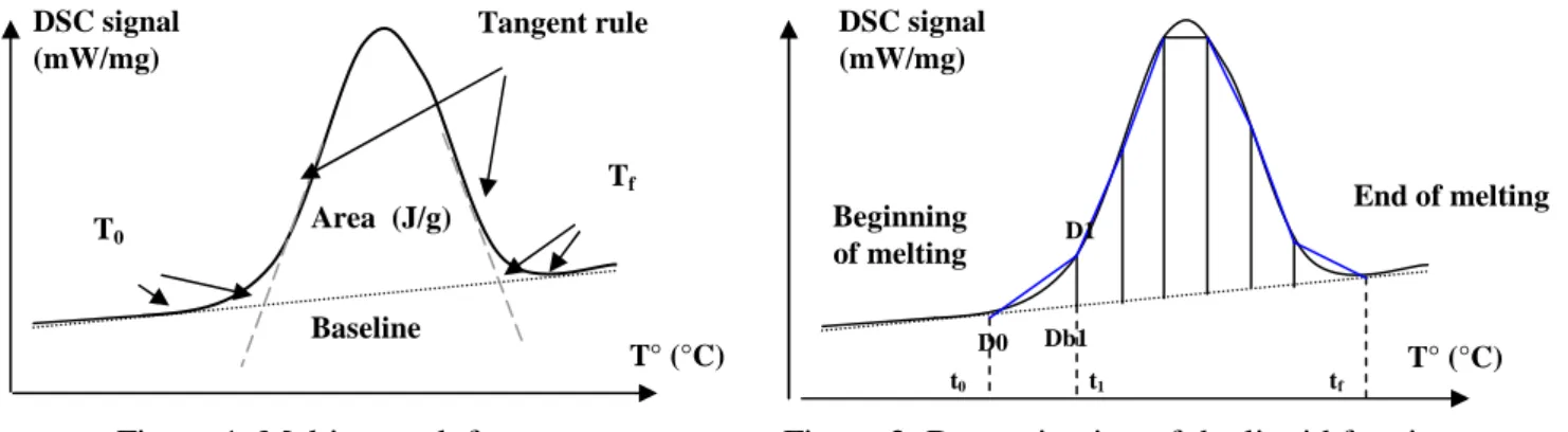
The applicability of a material for processing in the semi-solid state is defined by the solidus-liquidus interval and the development of liquid phase in the interesting temperature range. For the evaluation of the solidus and liquidus temperature a Differential Scanning Calorimetry (DSC) was used. The development of the liquid phase with increasing temperature was calculated using the values from the DSC-measurements. The evaluation of the liquid phase distribution is carried out by the application of a peak partial area integration. The whole area under the enthalpy-area curve is used to determine the melting enthalpy of the material. During DSC measurement, the typical melting peak obtained is shown in figure 1.
The peak characteristics are:
1) The changes of slope, jumps and peaks showing the thermal events (phase transformations, chemical reactions, etc..)
2) The peak area is the enthalpy variation of the transformation 3) The specific heat is calculated from the baseline
4) Solidus-liquidus interval: T end of melting-T beginning of melting (Tf - To)
We admit that the liquid fraction is proportional to the absorbed energy during the transformation. The sample is heated until total melting. Therefore, the liquid fraction can be calculated considering the peak area of the transformation, as shown in figure 2.
The characterisation of the melting peak is realised with the following parameters: 1) Total area ↔ 100% of the liquid fraction
2) Beginning and end of melting
The liquid fraction is determined with the following relation (1):
Area Total T T Area liquid ( i) % = 0 − (1)
2. Thermophysical Properties Characterization Dilatometry
The dilatometry is a technique used to measure the relative dilatation ∆L/L0 of a material submitted to a temperature program (∆L is the difference between the length at temperature T and the initial length L0 at room temperature).
T° (°C) DSC signal
(mW/mg)
tf
Figure 2. Determination of the liquid fraction .
Beginning of melting End of melting t0 t1 D0 Db1 D1 T° (°C) Tangent rule Baseline Area (J/g) T0 Tf DSC signal (mW/mg)
In our case, the sample holder for powder and pasty sample is required because we carried out the dilatation run tests for high temperatures, where the sample is in liquid state (figure 3).
Average Expansion Coefficient
From the dilatation values obtained and thanks to the relation (2), it was possible to calculate the average expansion coefficient CTE (T1-T2) for the temperature interval (T2 – T1).
(2)
Density
Density ρ(T) was calculated from the expansion values according to the following relation (3). (3)
where, ρ0: density at reference (mostly ambient) temperature
∆ L(T): expansion of the specimen under investigation L0 : specimen length at room temperature DSC-Cp Determination
DSC is a technique in which the difference in energy input into a substance and a reference material is measured as a function of temperature, while the substance and reference material are subjected to a controlled temperature program. Individual Cp values at different temperatures are determined using a sapphire as a standard according to the following equation (4).
(4) where, Cp: specific heat of the sample at temperature T
Cp, Standard: tabulated specific heat of the standard at temperature T mStandard: mass of the standard
mSample: mass of the sample
DSCSample: value of DSC signal at temperature T from the sample curve DSCstandard: value of DSC signal at temperature T from the standard curve
DSCBas: value of DSC signal at temperature T from the baseline
∆ + ∆ + ∆ + = 3 0 2 0 0 0 ) ( ) ( 3 ) ( 3 1 . ) ( L T L L T L L T L T ρ ρ 1 2 1 0 2 0 2 1 T T ) T ( L L ) T ( L L ) T T ( CTE − ∆ − ∆ = − where,
T2: upper temperature limit T1: lower temperature limit :length change relative to L0
0
L L ∆
Figure 3. Sample holder for powdery and pasty samples.
Standard P, Bas Standard Bas Sample Sample Standard P *C DSC DSC DSC DSC * m m C − − =
Thermal Diffusivity – Laser Flash
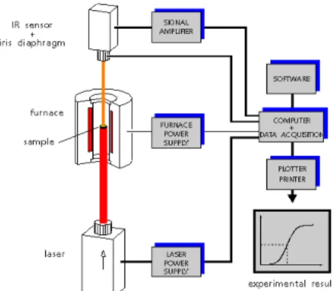
The front face of a cylindrically shaped piece is homogeneously heated by an unfocused laser pulse (figure 4). On the rear face of the test piece the temperature increase is measured as a function of time. The mathematical analysis of this temperature/time function allows the determination of the thermal diffusivity D(T) as presented in reference [4]. As we determined diffusivity till liquid state, we used a special quartz sample container.
Thermal Conductivity
Knowledge of thermal diffusivity D(T), density ρ(T) and specific heat Cp(T) allowed the determination of the thermal conductivity χ(T), calculated according the Laplace relation (5):
χ
(T)=D(T)*
ρ
(T)*C
p(T)
(5)Results
1. Solidus-Liquidus Interval and Fraction Solid Versus Temperature Characterization
Some basic alloys are studied and compared to modified alloys. The basic alloys are C38*, C80* and 100Cr6*. The modified alloys are C38 Asco modif 1* and C38 Asco modif 2*, 100Cr6 Asco modif 1*, 45Mn5 Asco modif 1* and 50Mn6 Asco modif 1*. All properties are compared to the base alloy C38. The base alloy C38 was used to study the effect of heating rate on DSC curves. The 50Mn6 Asco modif 1 alloy was used to study the homogeneity of the billet. The results are presented hereafter. Figures 6, 8, 10, 12, 14, 16, 18, 20, 22, 24, 26, 28 and 30 show the DSC signal of the melting peak and figures 7, 9, 11, 13, 15, 17, 19, 21, 23, 25, 27, 29 and 31 corresponding liquid fraction.
C38
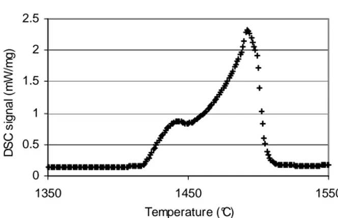
The DSC signal and the liquid fraction of C38 are shown in figures 6 and 7. Different heating rates were used (2°/min, 10°/min and 20°/min). The DSC curves show that the DSC signals increase with heating rate but the sensitivity and the peak separation decrease. For liquid fraction evolution, the results are similar for 10 and 20°/min. All subsequent experiments were therefore conducted with a heating rate of 20°/min. During melting of C38 we observed three different peaks which are related to the transformation:
* The composition follows euronorm DIN code. C38 = (carbon 0.38 %), C80 = (carbon 0.80 %), 100 Cr6 = (carbon 1 %, Cr 1.5 %), 50 Mn6 = (carbon 0.5 %, Mn 1.5 %), 45 Mn5 = (carbon 0.45 %, Mn 1 %).
Figure 5. Laser flash apparatus schematic. Figure 4. Laser pulse on the sample.
Laser Pulse
Temperature Signal Versus Time
1) γ→γ + liquid,
2) peritectic transformation γ + liquid →δ + liquid, and 3) δ + liquid → liquid
C80, C38
The DSC signal during melting and the liquid fraction of C80 are shown in figures 8 and 9. The comparison between C38 and C80 is shown in figures 10 and 11.
With regard to Kazakov parameters, C80 exhibits better behaviour than C38. The beginning of melting T0 is lower, T1 is lower, the solidification interval (Tf – T0) is larger (see table I), and the slope of the curve dF/dT is flatter at T1 and Tf.
Figure 6. DSC signal of C38. 0 0.2 0.4 0.6 0.8 1 1.2 1.4 1.6 1350 1450 1550 Temperature (°C) D S C s ig n a l ( m W /m g ) 20°C/mn 10°C/mn 2°C/mn
Figure 7. Liquid fraction of C38.
0 0.25 0.5 0.75 1 1350 1450 1550 Temperature (°C) L iq u id f ra c tio n 20°C/min 10°C/min 2°C/min Figure 8. DSC signal of C80. 0 0.2 0.4 0.6 0.8 1 1.2 1.4 1.6 1.8 1250 1350 1450 1550 Temperature (°C) D S C s ig n a l (m W /m g ) 0 0.25 0.5 0.75 1 1250 1350 1450 1550 Temperature (°C) L iq u id f ra c tio n
Figure 9. Liquid fraction of C80.
Figure 10. Comparison of the DSC signal between C38 and C80.
0 0.2 0.4 0.6 0.8 1 1.2 1.4 1.6 1.8 2 1250 1350 1450 1550 Temperature ( °C) D S C s ig n a l ( m W /m g ) C38 C80
Figure 11. Comparison of the liquid fraction between C38 and C80.
0 0.25 0.5 0.75 1 1250 1350 1450 1550 Temperature (°C) L iq u id f ra c tio n C38 C80
100Cr6, 100 Cr6 Asco modif 1, C38
The DSC signal and the liquid fraction of 100 Cr6 and 100 Cr6 Asco modif 1 are shown in figures 12, 13 and 14, 15 respectively. The C38, 100Cr6 and 100Cr6 Asco modif 1 results are shown in figures 16 and 17.
With regard to Kazakov parameters, 100 Cr6 Asco modif 1 exhibits better behaviour than 100 Cr6 and C38 one. The beginning of melting T0 is lower, T1 is lower, the solidification interval (Tf – T0) is slightly larger (see table I) and the slope of the curve dF/dT is flatter at T1.
0 0.5 1 1.5 2 2.5 1250 1350 1450 1550 Temperature (°C) D S C s ig n a l ( m W /m g )
Figure 14. DSC signal of 100 Cr6 Asco modif 1.
Figure 16. Comparison of the DSC signal between C38, 100 Cr6
and 100 Cr6 Asco modif 1.
0 0.5 1 1.5 2 2.5 3 1250 1350 1450 1550 Temperature ( °C) D S C s ig n a l ( m W /m g ) 100 Cr6 100 Cr6 Asco modif1 C38 0 0.25 0.5 0.75 1 1250 1350 1450 1550 Temperature (°C) L iq u id f ra c ti o n 100Cr6 100 Cr6 Asco modif 1 C38
Figure 17. Comparison of the liquid fraction between C38, 100 Cr6
and 100 Cr6 Asco modif 1. Figure 12. DSC signal of 100 Cr6. 0 0.5 1 1.5 2 2.5 3 1250 1350 1450 1550 Temperature (°C) D S C s ig n a l (m W /m g )
Figure 13. Liquid fraction of 100 Cr6.
0 0.25 0.5 0.75 1 1250 1300 1350 1400 1450 1500 1550 Temperature (°C) L iq u id f ra c tio n 0 0.25 0.5 0.75 1 1250 1350 1450 1550 Temperature (C°) L iq u id f ra c tio n
C38 Asco Modif 1, C38 Asco Modif 2, C38
The DSC signal and the liquid fraction of C38 Asco modif 1 are shown in figures 18 and 19. The DSC signal and the liquid fraction of C38 Asco modif 1 are shown in figures 20 and 21. The C38, C38 Asco modif 1 and 2 results are shown in figures 22 and 23.
With regard to Kazakov parameters, C38 Asco modif 2 exhibits better behaviour than C38 Asco modif 1 and C38 ones. The beginning of melting T0 is lower, T1 is lower, the solidification interval (Tf – T0) is slightly larger (see table I) and the slope of the curve dF/dT is flatter at T1 and Tf. 0 0.5 1 1.5 2 2.5 1350 1450 1550 Temperature (°C) D S C s ig n a l ( m W /m g )
Figure 18. DSC signal of C38 Asco modif 1.
0 0.25 0.5 0.75 1 1350 1450 1550 Temperature (°C) L iq u id f ra c ti o n
Figure 19. Liquid fraction of C38 Asco modif 1.
0 0.5 1 1.5 2 2.5 1350 1450 1550 Temperature (°C) D S C s ig n a l (m W /m g ) C38 C38 Asco modif1 C38 Asco modif2
Figure 22. Comparison of the DSC signal between C38, C38 Asco modif 1
and C38 Asco modif 2.
0 0.25 0.5 0.75 1 1350 1450 1550 Temperature (°C) L iq u id f ra c ti o n C38 C38 Asco modif1 C38 Asco modif2
Figure 23. Comparison of the liquid fraction between C38, C38 Asco modif 1
and C38 Asco modif 2. Figure 21. Liquid fraction of
C38 Asco modif 2. 0 0.25 0.5 0.75 1 1350 1450 1550 Temperature (°C) L iq u id f ra c ti o n 0 0.5 1 1.5 2 2.5 1350 1450 1550 Temperature (°C) D S C s ig n a l ( m W /m g ) Figure 20. DSC signal of C38 Asco modif 2.
45Mn5 Asco Modif 1 and C38
The DSC signal during melting and the liquid fraction of C38 Asco modif 1 are shown in figures 24 and 25.
The comparison between C38 and 50Mn6 Asco modif 1 is shown in figures 26 and 27. The conclusions are similar to the other alloys, the behaviour of 45 Mn5 Asco modif 1 is better than C38.
50Mn6 Asco Modif 1
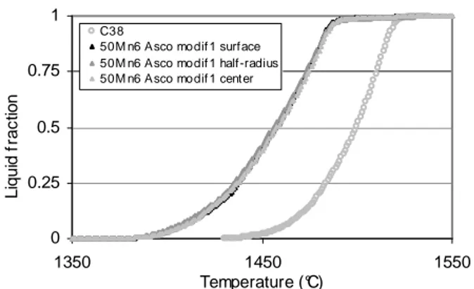
In order to determine the ingot homogeneity, three samples of 50Mn6 Asco modif 1 (named surface, half-radius and center) were taken and studied. These results are as follows (figures 28 and 29). They show that the behaviour of the ingot is rather homogeneous regarding liquid fraction. This is of course important for industrial practice.
Figure 26. Comparison of the DSC signal between C38 and 45Mn5 Asco modif 1.
0 0.5 1 1.5 2 1350 1450 1550 Temperature (°C) D S C s ig n a l ( m W /m g ) 45Mn5 Asco modif1 C 38 Figure 24. DSC signal of 45Mn5 Asco modif 1. 0 0.2 0.4 0.6 0.8 1 1.2 1.4 1.6 1.8 2 1350 1450 1550 Temperature (°C) D S C s ig n a l (m W /m g )
Figure 27. Comparison of the liquid fraction between C38 and 45Mn5 Asco modif 1.
0 0.25 0.5 0.75 1 1350 1450 1550 Temperature (°C) L iq u id f ra c ti o n 45Mn5 Asco modif1 C38
Figure 25. Liquid fraction of 45Mn5 Asco modif 1. 0 0.25 0.5 0.75 1 1350 1450 1550 Temperature (°C) L iq u id f ra c tio n 0 0.5 1 1.5 2 1350 1450 1550 Temperature (°C) D S C s ig n a l ( m W /m g )
50M n6 Asco modif 1 surface 50M n6 Asco modif 1 half-radius 50M n6 Asco modif 1 center
Figure 28. DSC signal of 50 Mn6 Asco modif 1. 0 0.25 0.5 0.75 1 1350 1450 1550 Temperature (°C) L iq u id f ra c tio n
50M n6 Asco modif 1 surf ace 50M n6 Asco modif 1 half-radius 50M n6 Asco modif 1 cent er
Figure 29. Liquid fraction of 50 Mn6 Asco modif 1.
The comparison between C38 and 50Mn6 Asco modif 1 is shown figures 30 and 31.
As regarding Kazakov parameters, the behaviour of 50 Mn6 Asco modif 1 is better than C38 one. The beginning of melting T0 is lower, T1 is lower, the solidification interval (Tf – T0) is slightly larger (see table I) and the slope of the curve dF/dT is flatter at T1 and Tf.
Alloys features during melting
Table I gives main characteristic temperatures and slopes of the liquid fraction curve during melting at 20°/min. Alloys are classified following decreasing T0.
Table I. Characteristic temperatures and slopes
Alloys T0 (°C) T1 (°C) Tf (°C) Tf - T0 (°C) Slope at T1 Slope at Tf
C38 1430 1500 1536 106 0.0200 0.0019
C38 Asco modif 1 1415 1478 1517 102 0.0185 0.0017
45 Mn5 Asco modif 1 1411 1470 1501 90 0.0173 0.0020
50 Mn6 Asco modif 1 (surface) 1389 1458 1519 130 0.0136 0.0002
50 Mn6 Asco modif 1 (half-radius) 1386 1456 1520 134 0.0127 0.0002
50 Mn6 Asco modif 1 (center) 1382 1456 1519 137 0.0139 0.0002
C38 Asco modif 2 1379 1472 1520 141 0.0145 0.0007
C80 1361 1450 1491 130 0.0114 0.0003
100 Cr6 1315 1431 1487 172 0.0111 0.0004
100 Cr6 Asco modif 1 1278 1402 1460 182 0.0097 0.0013
It is clear that for non alloyed steels the C38 Asco modif 2 gives the best results: T0 and T1 are lower, (Tf – T0) is larger, the slopes at T1 and Tf are lower than those of C38. It was used for the simulation of heating. Regarding low alloyed steels, 45 Mn 5 Asco modif 1 is not interesting. On the contrary 100 Cr6, 100 Cr6 Asco modif 1 and 50 Mn 6 Asco modif 1 show good behaviour.
2. Thermophysical Properties Characterisation
These properties were determined on the alloy C38 Asco Modif 2 and was used for the simulation of heating phase. The results of that simulation are shown in reference [5].
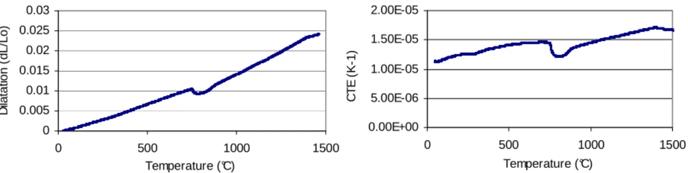
Dilatometry and CTE
The dilatation and CTE results are shown in figures 32 and 33. Table II gives values of the relative dilatation. 0 0.5 1 1.5 2 1350 1450 1550 Temperature (°C) D S C s ig n a l ( m W /m g ) C38
50M n6 Asco modif 1 surface 50M n6 Asco modif 1 half -radius 50M n6 Asco modif 1 center
Figure 30. Comparison of the DSC signal between C38 and 50 Mn6 Asco modif 1.
0 0.25 0.5 0.75 1 1350 1450 1550 Temperature (°C) L iq u id f ra c ti o n C38
50M n6 Asco modif 1 surface 50M n6 Asco modif 1 half-radius 50M n6 Asco modif 1 center
Figure 31. Comparison of the liquid fraction between C38 and 50 Mn6 Asco modif 1.
Table II. Relative dilatation during heating
Temperature (°C) Relative dilatation (∆L/Lo)
100 8.39E-04
500 6.65E-03
1000 1.41E-02
1500 2.45E-02
Density
The figure 34 shows the evolution of the density during heating in terms of temperature. The peak observed at 750°C is due to the phase transformation austenite-ferrite.
DSC-Cp Determination
The evolution of the specific heat versus temperature is shown in figures 35 and 36.
We can see a peak around 750°C. This is the phase transformation (austenite-ferrite) already seen from the dilatometry. The dramatic increase about 1400°C is due to the sample melting. The specific heat is directly calculated from the DSC curves. Therefore if a transformation Figure 32. Evolution of the dilatation during heating.
0 0.005 0.01 0.015 0.02 0.025 0.03 0 500 1000 1500 Temperature (°C) D ila ta tio n ( d L /L o )
Figure 33: Evolution of the CTE during heating.
0.00E+00 5.00E-06 1.00E-05 1.50E-05 2.00E-05 0 500 1000 1500 Temperature (°C) C T E ( K -1 )
Figure 35. Evolution of the apparent specific heat during heating.
0 5 10 15 20 0 500 1000 1500 Temperature (°C) A p p a re n t s p e c if ic h e a t (J /g K )
Figure 36. Evolution of the specific heat during heating.
0 0.4 0.8 1.2 1.6 2 0 500 1000 1500 Temperature (°C) S p e c if ic h e a t (J /g K ) 7.3 7.4 7.5 7.6 7.7 7.8 7.9 8 0 500 1000 1500 Temperature (°C) D e n s ity ( g /c m ³)
occurs during DSC measurement, it influences also Cp measurement. Figure 35 gives specific heat values if we take into account the quantity of heat ∆H released during the transformations, hence the y-axis title “apparent specific heat”. Ignoring the quantity of heat ∆H, we obtain the specific heat values shown in figure 36.
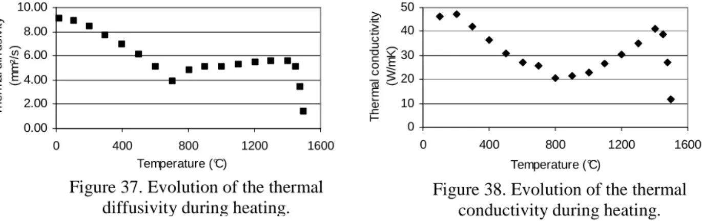
Thermal Diffusivity and Conductivity
The behaviour of the diffusivity during heating is shown below, figure 37. The thermal conductivity is shown in figure 38.
The behaviour of the thermal conductivity is similar to the thermal diffusivity. The values decrease until about 750°C. When the phase transformation occurs, the thermal conductivity increases until the beginning of melting. There is a dramatic diminution during melting, and the more liquid, the smaller the thermal conductivity.
Conclusions
The DSC measurements and corresponding liquid fraction versus temperature were used to study different alloys. For non alloyed steels, C38 Asco modif 2 shows better behaviour as regarding T0, T1, (Tf – T1) and dF/dT (T1, Tf) than C38. For low alloyed steels 100 Cr6, 100 Cr6 Asco modif 1 and 50 Mn6 Asco modif 1 show good behaviour. They could be chosen as candidates for thixoforming. Thermophysical properties characterisation are obtained on C38 Asco modif 2 (α, CTE, density, Cp, thermal diffusivity and thermal conductivity). These properties were used for the simulation of heating phase as presented in reference [5]. As regards to thermal conductivity, a dramatic diminution is observed during melting.
REFERENCES
1. H. Meuser, W. Bleck, “Determination of Parameters of Steel Alloys in the Semi-Solid State,”
Procedings of Semi-solid Processing, (2002), 349.
2. H.V.Atkinson, P. Kapranos, D.H. Kirkwood, “Alloy Development for Thixoforming,”
Procedings of Semi-solid Processing, (2000), 445-446.
3. A.A. Kazakov, “Alloy Compositions for Semisolid Forming,” Advanced Materials &
Processes, (2000), 31-34.
4. J. A. Cape, G.W. Lehman, “Temperature and Finite Pulse-Time Effects in the Flash Method for Measuring Thermal Diffusivity,” Journal of Applied Physics, 37 (1963), 1909.
5. A. Rassili et al., “Improvement of Materials and Tools for Thixoforming of Steels,”
Proceedings of Semi-solid Processing, (2004).
Figure 37. Evolution of the thermal diffusivity during heating.
0.00 2.00 4.00 6.00 8.00 10.00 0 400 800 1200 1600 Temperature (°C) T h e rm a l d if fu s iv it y (m m ²/ s )
Figure 38. Evolution of the thermal conductivity during heating.
0 10 20 30 40 50 0 400 800 1200 1600 Temperature (°C) T h e rm a l c o n d u c tiv ity (W /m K )