Adaptive control design with guaranteed margins for nonlinear plants

Adaptive Control Design with Guaranteed

Margins for Nonlinear Plants

by

Jinho Jang

B.S., Seoul National University (2003)

S.M., Massachusetts Institute of Technology (2005)

MASSACHUSETTS INSTIUTE

ri-O)F TECH:NOLOGY

SMAR 0

6 2009

L IBRARIES

Submitted to the Department of Mechanical Engineering

in partial fulfillment of the requirements for the degree of

Doctor of Philosophy in Mechanical Engineering

at the

MASSACHUSETTS INSTITUTE OF TECHNOLOGY

February 2009

@

Massachusetts Institute of Technology 2009. All rights reserved.

A uthor ...

Dpartment of Mechanical Engineering

February, 2009

Certified by...

Anuradha M. Annaswamy

Senior Research Scientist

Thesis Supervisor

Accepted by ...

" "

David E. Hardt

Professor of Mechanical Engineering

Chairman, Department Committee on Graduate Students

Adaptive Control Design with Guaranteed Margins for

Nonlinear Plants

by

Jinho Jang

Submitted to the Department of Mechanical Engineering on November 18, 2008, in partial fulfillment of the

requirements for the degree of

Doctor of Philosophy in Mechanical Engineering

Abstract

Adaptive control is one of the technologies that improve both performance and safety as controller parameters can be redesigned autonomously in the presence of uncer-tainties. Considerable research has been accomplished in adaptive control theory for several decades and a solid foundation has been laid out for stability and robustness of adaptive systems. However, a large gap between theory and practice has been an obstacle to transition theoretical results into applications and it still remains. In or-der to reduce the gap, this thesis presents a unified framework for design and analysis of adaptive control for general nonlinear plants.

An augmented adaptive control architecture is proposed where a nominal con-troller is designed in the inner-loop with an adaptive concon-troller in the outer-loop. The architecture is completed by addressing three separate problems. The first prob-lem is the design of adaptive control in the presence of input constraints. With a rigorous stability analysis, an algorithm is developed to remove the adverse effects of multi-input magnitude saturation. The second problem is the augmentation of adaptive control with a nominal gain-scheduling controller. Though adaptive con-trollers have been employed with gain-scheduling to various applications, no formal stability analysis has been developed. In the proposed architecture, adaptive control is combined with gain-scheduling in a specific manner while stability is guaranteed. The third problem is the development of analytic stability margins of the closed-loop plant with the proposed adaptive controller. A time-delay margin is derived using standard Lyapunov stability analysis as an analytic stability margin.

The overall adaptive control architecture as well as the analytically derived mar-gins are validated by a 6-DoF nonlinear flight dynamics based on the NASA X-15 hypersonic aircraft. Simulation results show that the augmented adaptive control is able to stabilize the plant and tracks desired trajectories with uncertainties in the plant while instability cannot be overcome only with the nominal controller. The time-delay margins are validated based on a generic transport model and they are compared with margins obtained from simulations studies. We utilize numerical methods to find less conservative time-delay margins.

Thesis Supervisor: Anuradha M. Annaswamy Title: Senior Research Scientist

Acknowledgments

I am deeply indebted to my research adviser, Anuradha M. Annaswamy, for her

patient guidance and support for this thesis in the form of ideas, financial support, and moral support. She offered me the opportunity to carry out this research in the area that motivated me most. With a busy schedule, she has been always responsive and supportive to my requests, and always provided great ideas about my research. She has read each chapter with great care, often under extreme time pressure and made this thesis possible by her comments.

My sincere appreciation also goes to Eugene Lavretsky, John J. Leonard, and

Jonathan P. How for being my thesis committee members and for their research advice, thorough readings, and corrections. I am really grateful for the particular help of Zachary T. Dydek in implementing the nonlinear simulation model of NASA X-15. I am grateful to many of lab colleagues, in particular, Yildiray Yildiz, Travis E. Gibson, and Megumi Matsutani for sharing research ideas. Great thanks need to go to all graduate students and research scientists in Active Adaptive Control Laboratory who gave me helpful feedback on my studies: Jeajeen Choi, Himani Jain, Paul A. Ragaller, Manohar B. Srikanth, Seunghyuck Hong, Chun Yang Ong, and Hanbee Na.

All my love and thanks sincerely goes to families and parents for believing in me

and supporting me. They has always encouraged me to try my best and to achieve what I have dreamed. Particularly, I would like to thank my dearest Sunwoo Kim for her love, patience, and understanding from the bottom of my heart. My daughter, Jennifer Jang, gave me luck as well as high motivation to complete my study. And, last but not least, I have to thank God for giving me the second chance to study at MIT. I would not had this special chance without Him, and could not have made without Him.

Contents

2.1.1 Adaptive control in Magnitude Saturation . ... . . 26

2.1.2 Stability Margins in Adaptive control . ... 27

2.2 Gain-scheduling ... 27

3 Adaptive Control in the Presence of Multi-input Magnitude Satu-ration 29 3.1 Problem Statement ... 30

3.1.1 Plant with Uncertainties ... 30

3.1.2 Augmentation with Integral Action . ... 30

3.1.3 Multi-input Saturation ... 31

3.2 Adaptive Controller ... 33

3.2.1 Nominal Controller and Reference Model Design ... . 33

3.2.2 Adaptive Controller design . ... . 34

3.2.3 Proof of Bounded Tracking - Elliptical Saturation ... . 37

3.3 Sim ulation ... ...

3.3.1 Nominal Controller Design . . . . 3.3.2 Adaptive Controller Design . . . . 3.3.3 Simulation Results ...

3.4 Sum m ary ...

4 Adaptive Gain-scheduled Controller

4.1 Problem Statement ... .. 4.1.1 Linear Time-varying System . . . . 4.1.2 Augmentation with Integral Actions . . 4.2 Adaptive Controller ... . ...

4.2.1 Reference Model and Baseline Controller 4.2.2 _{Adaptive Controller Design . . . .} 4.3 Stability Analysis ... .. 4.4 Sim ulation ... ... ... ... ...

4.4.1 _{Nominal Controller Design . . . .} 4.4.2 Adaptive Controller Design . . . . 4.4.3 Simulation Results . . . . 4.5 Sum m ary ... . . . . . 51 .. . . . . 51 .. . . . . 53 . . . . 54 . . . . 59 61 . . . . 62 . . . . . 62 . . . . . 66 . . . . . 67 Design . ... 67 . . . . . 68 . . . . . .. . 70 . . . . . 74 . . . . . . . . 75 .. . . . . 79 . . . . . . . 79 . . . . 83

5 Stability Margins for Adaptive Control delay 5.1 Problem Statement ... 5.2 Adaptive controller ... in the Pr 5.2.1 Nominal controller and reference model design 5.2.2 Adaptive controller design ... 5.3 Delay M argins ... 5.3.1 _{(1,1) Pade approximation . . . ..} 5.3.2 _{(n,n) Pade approximation . . . ..} 5.4 Sim ulation . . . . esence of Time-87 . . . . 88 . . . . 90 . . . . . 90 . . . . 91 . . . . 92 . . . . . 93 . . . . 102 . . . 103

5.4.2 Delay Margins in First Order Plants . ... 107

5.4.3 Time delay and the Pade approximations . ... 113

5.4.4 Delay Margins in a Generic Transport Model (GTM) .... . 117

5.5 Summary ... 118

6 Summary and Future Work 121 6.1 Sum m ary ... .... . .. .. .. .. . .. . 121

6.2 Future W ork ... 123

A NASA X-15 Hypersonic Aircraft 127 A .1 History . . . .. . . . .... .. 127

A.2 X-15 Flight Dynamics Model ... 128

A.2.1 Equations of Flight Dynamics ... .. . 128

A.2.2 Aerodynamic Data ... 130

A.2.3 Actuators and Sensors ... 133

B Proofs and Constants 135 B.1 Proof of Proposition 4.1 ... 135

List of Figures

1-1 The illustration of the X-43A: A hypersonic and scramjet-powered

re-search aircraft [4]... 19

3-1 Elliptical and rectangular multi-input saturation functions ... 34 3-2 A schematic of the level set B and the region of attraction A... 40 3-3 The control input, 1, saturated by the rectangular saturation can be

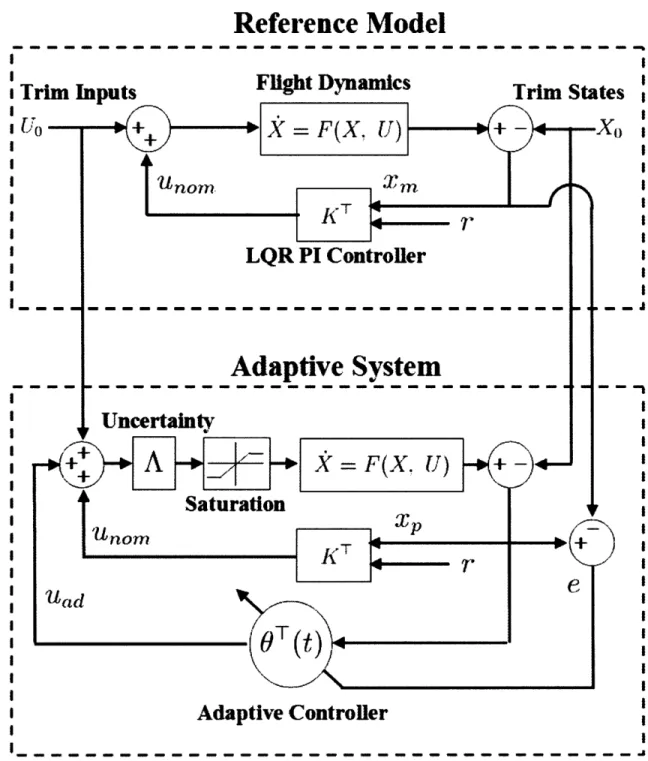
decomposed into Ud and i. ... 49 3-4 The block diagram of the reference model and the overall control

ar-chitecture in nonlinear simulation. . ... . 55

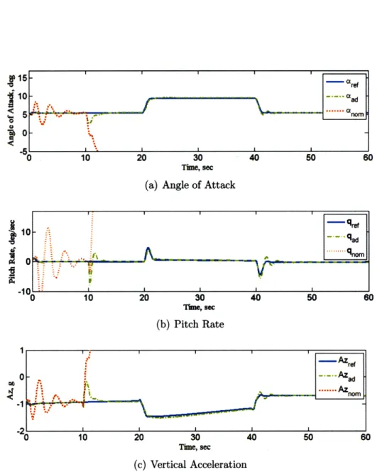
3-5 Response of angle of attack, pitch rate, and vertical acceleration of

reference (ref), adaptive (ad), and nominal (nom) systems under Ai.. 56

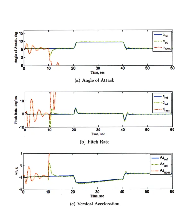
3-6 Response of angle of attack, pitch rate and vertical acceleration of reference, adaptive, and nominal systems under A2.. . . . . . 57 3-7 Response of angle of attack, pitch rate, and vertical acceleration of

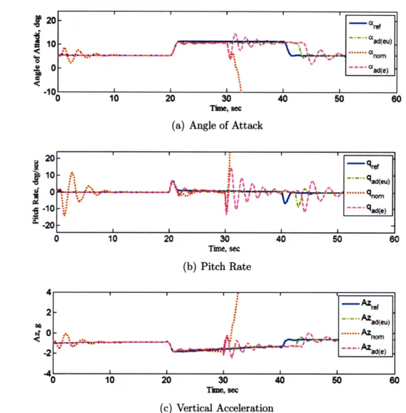
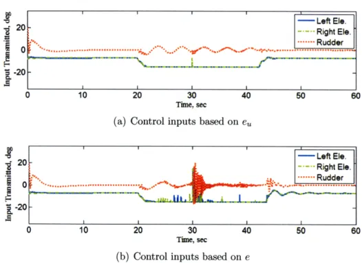
reference, adaptive, and nominal systems under A3.. . . . . . 59 3-8 Control inputs transmitted to the aircraft. . ... . 60

4-1 A block diagram of a multi-rate plant. Fast states and slow states are

controlled separately... 62

4-2 A schematic of trim points inside the operating envelope in the Xg space. 63 4-3 This figure illustrates the construction of desired states, X*(t)... . 64 4-4 Gain-scheduling strategy: linear mapping from online mearsurement

of Xg(t) to the offine gain table ... 69 4-5 Trim points and commands (hmd, Vmd) on the V - h space... 76

4-6 Profiles of altitude and velocity commands . ... 77

4-7 Poles of the open-loop plants and the reference models . ... 78 4-8 Velocity and altitude command-following in the presence of the

uncer-tainty, A... ... 80

4-9 State variables of the closed loop systems and the reference model . 81 4-10 Control surfaces of the closed loop systems and the reference model 82 4-11 State variables of augmented and non-augmented adaptive control . 84 4-12 Control surfaces of augmented and non-augmented adaptive control 85

5-1 Time-delay approximation ... ... 89 5-2 Two mutually exclusive cases in the cubic polynomial f(z) ... 100

5-3 The cubic polynomial, f(z), with T > Tm, 7 = Tm, and T < Tm,. .... 102

5-4 Analytically guaranteed and simulation-based margins with A = 0.5, Aa = 0.4, and Aq = 1 ... 106 5-5 Analytically guaranteed and simulation-based margins with A = 0.5,

Aa = -0.2, and Aq = 1 ... . ... 107 5-6 M ultipliers . ... ... ... ... .... ... . .. .. ... 110 5-7 Bounded (left) and unbounded (right) sets of attraction. ... 111 5-8 The region where G(e, 0, r1) > 0 is shaded in blue. A bounded set of

attraction exists when 7 = 0.081 (left) but there is no bounded set for

T= 0.082. ... . .. ... 112

5-9 The region where V(e, 0, yj) > 0 is shaded in blue. A bounded set of attraction exists when T = 0.15 (left) but there is no bounded set for

T =0.16 ... ... 112

5-10 Phase plot of time-delay and the Pade approximations. ... 114 5-11 Phase plot of time-delay and (1, 1) Pade approximation (T = 0.15). 115 5-12 Control input signal (above) with the delay (T = 0.15) and the

ampli-tude spectrum of the control input (below) . ... 116 5-13 Planform of the C-5A aircraft [11] . ... . 117

A-2 The full nonlinear X-15 aircraft model . ... 129 A-3 Planfrom of the X-15 hypersonic aircraft [12]. . ... . 131 A-4 Lift and drag coefficients [13]. . ... ... 132

List of Tables

3.1 Trim conditions and inputs. ... 52

5.1 Analytic and simulation-based margins for the first order plant when y =0.5, 1, 2, 5and a = 0.5. ... .. 113 5.2 Analytic margins with the Pade approximation. departing frequencies,

and dominant frequencies in control input . ... 116 5.3 Analytic and simulation-based margins for the short period dynamics

of C-5A when y = 2, 3, 4, 5, 10 and a = 0.5. ... 118

Chapter 1

Introduction

1.1

Motivation

Control design and analysis for systems with static and dynamic uncertainties, while operating in the presence of environmental disturbances and other unknown factors, present significant challenges. A classical fixed-gain controller can handle plant pa-rameter variations and disturbances to a certain degree. There exists an assortment of fixed control design methodologies and analysis tools for a physical system whose model is properly known. However, mathematical models of physical systems are generically imprecise and quite often simplified. In order to accommodate a larger class of uncertainties and to achieve higher performance, it is necessary to design ad-vanced active control algorithms. This need becomes especially important for safety critical applications whose performance requirements are steeper and more stringent. Another instance which mandates advanced controllers is in the context of un-manned autonomous flight systems, where the need for accurate performance is em-phasized because the human operator is not directly in the control loop and action through remote operators may not be sufficiently swift. Recent years have witnessed a variety of autonomous systems in both civilian and military applications that need to cope with unexpected situations without remote assistance. The application of adaptive control to those systems has been sought after in order to obtain benefits in safety, survivability, and performance as an enabling technology. However, one of

the early attempts at implementations of adaptive approaches in flight control led to an accident [13] which is due to a lack of understanding of adaptive systems and an implementation based on empirical rather than a theoretically validated design. This triggered an extensive investigation of a fundamental adaptive control theory.

Aside from plant uncertainties and safety requirements, most of dynamic systems are generically nonlinear. Unlike linear systems, nonlinear systems possess more com-plexities, one of which is the possible existence of multiple equilibrium points. In a high performance vehicle such as the X-43A (Figure 1-1), this characteristic becomes more dominant with the vehicle exhibiting different dynamic characteristics over mul-tiple equilibrium points. In addition, the equilibrium points are distributed over a large operating envelope. It is safe to say that while a general method exists for the control of linear plants, no universal method exists for the control of nonlinear plants.

Therefore, it is not surprising that the level of success of a given nonlinear control method, which in turn is predicated on certain assumptions, depends on how reason-able the assumptions made are in a given application. In this thesis, the nonlinear control method used is based on gain-scheduling. An adaptive controller is augmented with the gain-scheduling controller, which enables us to handle both uncertainty and nonlinearity concurrently. The augmented adaptive control is, therefore, expected to enhance the tracking performance.

In the application of adaptive control, important issues arise due to constraints on the plant inputs, such as actuator magnitude saturation. While performing aggressive and safety-required missions, input constraints can impair the overall performance of adaptive control and potentially cause instability in the closed-loop system. Particu-larly, in the presence of uncertainties, the adverse effects of input constraints tend to grow such that instability can occur in closed-loop adaptive systems while adaptation is actively performed on uncertain parameters. This necessitates a formal method to compensate input saturation in adaptive control design and a stability analysis.

While improving the performance in the presence of uncertainties, the augmented adaptive control should also maintain its robustness with respect to perturbations. It is well known that an adaptive system is in the most vulnerable situation when the

Dryden Flight Research Center ED98-44824-1 X-43/Hyper -X aircraft. NASA/Dryden Illustration by Steve Lighthill

Figure 1-1: The illustration of the X-43A: A hypersonic and scramjet-powered re-search aircraft [4].

adaptation is actively processed. For example, adaptation can cause divergence of the adaptive parameters when disturbances are present. To prevent instability and enhance the robustness of the adaptive control, significant efforts and, hence, principal achievements in the robust adaptive control theory were made in 1980s [27], which include modifications of the adaptive law and persistent excitation of the reference input. Unfortunately, no formal link has been developed between the robust adaptive control theory and its application to a specific problem such as aircraft control. In order to utilize the adaptive control scheme to realistic applications, it is necessary to develop analytical tools to measure and quantify its robustness. Furthermore, effects of design parameters in the adaptive controller on its robustness should be investigated extensively to transition the adaptive control theory to realistic applications. It is therefore highly required to develop analytic margins for adaptive systems to be aware of the level of perturbations that the adaptive systems are guaranteed to be stable.

1.2

Research Objectives

The research objective of this thesis is to provide a unified framework for the design and analysis of adaptive control architectures for nonlinear plants which are suscep-tible to parametric as well as non-parametric uncertainties, and deliver improved performance. The proposed research will concentrate on control design, stability / robustness analysis, as well as the development of Verification and Validation (V&V) methods, while using high fidelity 6-DoF nonlinear aircraft models. Specific problems that we shall address are:

o Adaptive control in the presence of multi-input saturation

Control of plants with constrained inputs is a theoretically challenging problem and one of paramount practical importance since actuator subject to saturation is ubiquitous in control applications. Constrained actuators can degrade per-formance and potentially lead to instability if they are not taken into account in control design. In particular, adaptive control technique can destabilize the overall system especially when "adaptation" is carried out on saturation error. As a remedy to prevent instability due to saturation, compensation methods have been introduced and we extend this method to multi-input case where the adaptive control is placed in an augmentation with the nominal controller that includes integral action. The first problem in this thesis is to develop a compensation method for multi-input saturation in adaptive control design.

* Adaptive control for nonlinear plants via integration of gain-scheduling

Significant characteristics of high performance nonlinear plants is that (i) they have multiple equilibrium points over a large operating envelope and (ii) they are generally multi-rate systems whose states have a broad spectrum of convergent or divergent rates. Obviously, characteristics of a nonlinear plant can vary con-siderably between equilibrium points. To achieve desired performance uniformly across operational envelope, a gain-scheduling controller can be constructed on nominal parameters by employing slow-rate states as gain-scheduling variables

[32, 26]. In order to maintain the performance in the presence of uncertain-ties, we propose to augment the gain-scheduling controller with an adaptive controller. The second specific problem is to arrive at a set of formal sufficient conditions that guarantee closed-loop stability and uniform performance.

* Analytical stability margins equivalent to linear concepts

Even though adaptive systems have been extensively studied over the past 40 years, their transient performance and robustness properties remain an open problem. What is needed here are theoretically verifiable techniques to ana-lyze and predict sensitivity to various uncertainties for systems with adaptive controllers. Currently, the chief obstacle to transitioning adaptive controllers into safety-critical applications is a lack of formal methods to assess stability / robustness margins with respect to static uncertainties, and unmodeled dynam-ics, such as time-delays. The third problem dealt in this thesis is to develop formal methods for calculation of stability / robustness margins for nonlinear systems operating with adaptive controllers in the loop. This will contribute to Verification and Validation (V&V) techniques for adaptive systems.

1.3

Research Approach

The approach adopted in this thesis to control a nonlinear plant in the presence of uncertainties is composed of the following three major steps:

The first step is the characterization and modeling of plausible uncertainties in nonlinear plants. Aside from numerous "unknown" uncertainties in reality, "known" uncertainties in such plants include control failures, sensor failures, input saturation, and unmodeled dynamic such as actuator dynamics, structural vibration, time-delay, and so on. They should be modeled and incorporated to the plant in a physical sense to replicate the real ones. In this step, we will form the overall plant model to be controlled in this research.

controller is augmented with a nominal controller. The reason is that there is always some prior information available, and this information can be used such that stability and uniform performance are obtained in the absence of uncertainties. The next component in the proposed architecture is the inclusion of gain-scheduling. In order to accommodate a range of equilibrium points, the nominal controller is designed using gain scheduling. This is accomplished by designing the fixed controller at each equilibrium point, resulting in a family of fixed controllers for an entire operating envelope. The gain scheduling is carried out using slow variables such as the velocity and height of the aircraft. In the outer loop of the nominal controller, the adaptive controller is included to accommodate uncertainties. The structure of the adaptive controller is determined so as to accommodate both parametric and non-parametric uncertainties.

In the third step, stability and robustness analysis of the complete closed-loop controller that consists of the gain-scheduled nominal controller in the inner-loop and the adaptive controller in the outer-loop is carried out. In the presence of both parametric and nonparametric uncertainties, the stability of the closed-loop system is analyzed. Computable measures of robustness margins where stability is guaranteed are also provided in the thesis.

To demonstrate performance of the proposed controller in simulation studies, a 6-DoF nonlinear model of the hypersonic aircraft (NASA X-15) is utilized to demon-strate performance of the proposed controller. To reconstruct the model fully, we will collect aerodynamic design and data from the literature, which will be incor-porated into nonlinear flight dynamic equations. For controller design purposes, we will linearize the nonlinear flight dynamics and obtain a family of operating points for which linearized dynamics are defined. Once the controller designed, it will be tested with the nonlinear model. In order to examine performance of the proposed controller extensively, a great deal of uncertainties and unmodeled dynamics will be tested with a set of different free parameters of the adaptive controller. Through simulation and suitable analytical studies, we will quantify the worst uncertainties for a given controller and specified commands.

1.4

Organization

This thesis is divided into six chapters. The contents of chapters are summarized as followed:

* Chapter 1, Introduction, motivates the research effort, and introduces the re-search objectives as well as specific problems delivered. It also describes the research approaches adopted in this thesis.

* Chapter 2, Background, discusses previous works dealing with adaptive control theories and applications. In this chapter, the review of gain-scheduling methods and its applications are also stated.

* Chapter 3, Adaptive Control in the Presence of Multi-input Magnitude

Satura-tion, discusses a stable method to compensate saturation of multiple inputs in

the adaptive control design.

* Chapter 4, Adaptive Gain-scheduled Controller, addresses the problem of con-trolling a nonlinear system in the presence of parametric uncertainties. The proposed adaptive controller includes a nominal controller which is based on gain-scheduling to accommodate dynamic characteristic changes over multiple equilibrium points.

* Chapter 5, Stability Margins for Adaptive Control in the Presence of

Time-delay, presents an analytical tool to quantify robustness margins of the adaptive

controller with guaranteed stability.

* Chapter 6, Conclusion, discusses the results and summarizes the thesis work. The topics for future works are proposed based on these conclusions accordingly.

Chapter 2

Background

This chapter presents the theoretical background on adaptive control and explains its applications to dynamic systems. It then reviews the related previous works of adaptive flight control when adaptive control inputs are constrained in magnitude. Literatures on gain-scheduling are also reviewed.

2.1

Adaptive Control: Theory & Applications

One of the main characteristics than generally distinguishes adaptive control from earlier control architectures is that the former monitors the performance of the over-all plant and uses the information obtained to update the control law automaticover-ally and on-line so as to improve performance. This fundamental idea underlying adaptive control dates back to mid-1950s when flight control was a source of driving force. In 1960s, several adaptive control schemes were developed an they include self-oscillating adaptive system (SOAS), model reference adaptive control (MRAC), and self-turning regulator (STR). The SOAS designed by Honeywell has been tested on the NASA X-15 hypersonic aircraft, resulting in a catastrophic result in November, 1967 [13]. Due to the crash of the test flight, interest in the adaptive control moved to stability analysis and from late 1970s to early 1980s, a systematic theory with guaranteed sta-bility and performance emerged, and this resulted in outgrowth of publications and several books [28, 1, 15, 33, 23, 39] by the mid 1990s. Along with stability analyses,

the robustness of adaptive control was extensively studied in 1980s since nonparamet-ric uncertainties could destabilize adaptive systems [6, 14]. Several robust adaptive control methods were developed to improve the performance of adaptive controllers in the presence of disturbances and unmodeled dynamics [28, 15]. Extensions to nonlinear control methods have been addressed extensively in [36, 22].

Aligned with theoretical achievements, in various engineering applications such as ships, automotive systems, robot manipulators, and power systems, process con-trols, adaptive control architectures have been utilized and proved to be suited for performance improvement. It is interesting to note that an adaptive controller was designed for a tailless fighter research aircraft, the X-36, and a test flight was carried out in 1998 [41], resulting in satisfactory performance and guaranteed stability.

2.1.1

Adaptive control in Magnitude Saturation

Adaptive control approaches for plants with constrained inputs in magnitude have been developed and introduced in [19, 2, 5, 38, 17, 24]. In [19], Karason and An-naswamy introduced a saturation compensation method for direct-adaptive control and showed that for a single input plant with output feedback, bounded trajectories can be guaranteed for a range of initial conditions whether the open-loop plant is stable or not. Cheng and Wang in [5] reviewed the current methods to compensate magnitude saturation in adaptive control. Most of those methods relied on the as-sumption that the open-loop plant is stable. Strategies for input saturation in indirect adaptive control were discussed in [38] for open-loop stable plants. In [17], Johnson and Calise developed a method to compensate limitation on the plant inputs when neural network adaptive control is designed. Recently, in [34], these results were extended to the case of a multi-input plant where an elliptical multi-input satura-tion funcsatura-tion is employed. This results showed that boundedness of all signals in the closed-loop system is bounded when initial conditions lie in a compact set. In [24]. Lavretsky presented a modification of [19] such that stable adaptation is achieved without hard actuator saturation. Instead of the artificial saturation function where inputs are constrained elliptically, a realistic multi-input saturation function was

uti-lized in [24].

2.1.2

Stability Margins in Adaptive control

Though adaptive systems have been extensively studied over the past three decades as we mentioned above, it should be noted that theoretically justifiable Verification and Validation (V&V) techniques for adaptive systems are absent. Current V&V techniques are subject to the constraint that the underlying control design is linear [10], which is inadequate for adaptive flight control systems. This may be a demanding task because adaptive systems are generically nonlinear. For example, there is no technique to quantify the level of time-delays that adaptive systems can withstand. Similarly, there is no tool to determine how far or close adaptive systems are situated from instability conditions. Absence of analytical technique for stability / robustness margins has been an obstacle to applying adaptive control theory to safety critical applications such as flight control.

2.2

Gain-scheduling

One of the promising methods for nonlinear control design is gain-scheduling [32, 26] which extends design-via-linearization approach to a range of equilibrium points [20]. It has been used in a wide range of applications including flight control [29], chemical process control [30], and wind-turbine control [25] since 1950s. Historically, gain scheduling has been considered as a "practitioner's" technique. It is therefore not surprising that most of the literature in this area, before 1990s, dealt with practical applications. Theoretical approaches to gain scheduling in terms of design, analysis, and implementation has commenced thereafter [35, 18, 31].

The main idea behind the gain-scheduling approach is to decompose the nonlinear control design task into a family of linear control design methods and scheduling this family of linear controllers based on the command signal so as to ensure that the original nonlinear system is suitably controlled. One or more measurable variables, called gain-scheduling variables, are utilized to determine what operating region the

system is currently in and to enable the appropriate linear controller designed for that region. When gain-scheduling variables are slowly varying, stability results of almost time-invariant systems can be called upon to establish the stability of the underlying linear time-varying system and therefore the closed-loop system that involves the original nonlinear system [32, 26]. The attractive feature of gain-scheduling is that it simply uses linear design tools to nonlinear systems so that a diversity of linear design methodologies can be employed. However, there are still several ad-hoc processes in designs and problem formations which are acceptable in simple applications, but troublesome in complicated ones.

The design of gain-scheduled controller can be broadly partitioned into four steps [32]. In the first step, a linear model parametrized by gain-scheduling variables needs to be obtained. The most common method is based on Jacobian linearization on a family of equilibrium points, particularly called trim points in flight control. This generates a family of linearized plants. The second step is to design linear controllers for those linearized plants such that for each frozen value of gain-scheduling variable, the closed-loop system with the corresponding linear controller shows satisfactory performance. Then, the off-line table of controller gains is built based on the gain-scheduling variables. In the third step, the gain-gain-scheduling is executed so that the controller gain is varied based on the current value of the gain-scheduling variables. Historically, an interpolation process has been used to schedule the controller gains. The fourth step is stability analysis and performance test which is subject to simula-tion studies.

In an aircraft flight control system, the altitude (or dynamic pressure) and Mach number (or velocity) have been used as scheduling variables conventionally, which are slowly varying variables compared to aero-angles and rates [32, 26].

Chapter 3

Adaptive Control in the Presence

of Multi-input Magnitude

Saturation

This chapter investigates the design of an adaptive controller in the presence of mul-tiple actuator saturation as well as uncertainties. An augmented control architecture is proposed where the adaptive controller is designed in the outer-loop of a fixed PI controller which serves as a baseline control. In order to avoid the adaptive controller parameters to be misleadingly adjusted by the saturation error, we utilize the aug-mented error method in the adaptive control design that Karason and Annaswamy developed in [19] for SISO systems and provide the stability analysis rigorously. The overall controller is proved to result in semi-global boundedness with respect to the size of saturation limits in the sense that the region of attraction extends to the entire space as the the saturation level decreases. To perform more realistic simulation stud-ies, we reconstruct a nonlinear model of the NASA X-15 hypersonic aircraft based upon aerodynamic data in [13]. Theoretical findings are validated with simulation studies through this model with realistic actuator constraints and failures. Simulation results show that adaptive control stabilizes the closed-loop system and tracks the reference model properly while the nominal controller is unable to overcome insta-bility. Compensation for magnitude saturation is proven to be useful to avoid high

oscillation in the adaptive control inputs due to saturation errors.

3.1

Problem Statement

3.1.1

Plant with Uncertainties

The problem is under consideration is the control of a linear plant of the form

S= Ax + Bu

(3.1) y = Cx

where x E R' is the state, u E Rm _{is the control input, and y E R1 is the output of the}

plant with 1 < m. A E R x n

, B E R]xm, and C E R"lx are a known system, input, and output matrix respectively. When there exist uncertainties and disturbances in the plant in (3.1), we consider a plant in the form of

, = Ax + BA(u + d) (3.2)

y = Cz

where A c IRx"n is an unknown system matrix. A Rmxm is an unknown diagonal

matrix which represents actuator anomalies such as uncertainties, loss of control ef-fectiveness, and reversal in the control input. Ai denotes the ith element of A. For the purpose of control design, we assume that the followings hold:

Assumption 3.1. (AA, BA) is controllable.

Assumption 3.2. The sign of Ai, denoted by sgn(Ai), for i = 1,... , m is known.

3.1.2

Augmentation with Integral Action

The goal of the control design is that the output tracks a given command signal despite the the presence of uncertainties and disturbances. Toward this goal, we

design an inner-loop controller that integrates the output tracking error as

.c = B,(y - r) (3.3)

where x, E Rnc is the controller state and r E R' is the command signal such that

Ilrll <

con-troller is wriiten as =[ + A(u + d) + r (3.4) xc BcC Oncxnec ncxm -B hp A xp Bp B2 or equivalently as k, = A, x, + BplA(u + d) + BP2r (3.5) where xp, RWn _{, Ap E Rn} x n_p , _{Bpl E Rnpxm, and BP}

2 E Rn x . Oixy denotes the i x j

zero matrix. The controllability of the pair (Ax, B) is not sufficient for that of the pair (ABA, Bp1) so that the following assumption is required [7]:

Assumption 3.3.

A B

BcC

3.1.3

Multi-input Saturation

The inputs from actuators to the plant in (3.2) are constrained in magnitude. We, therefore, introduce two multi-dimensional saturation functions: elliptical and rect-angular saturation functions.

Definition 3.1. The function, E,(-), is an elliptical multi-dimensional saturation function defined by

E.(u) = u1 if IuI < ge(U) (3.7)

where ge(u) is given by

Fm \i 2 -1/2

i

/

e^ = u/lull denotes the unit vector in the direction of u, Ui,mx is the saturation limit of the ith actuator, and ui is given by

U = 6g(u).

Definition 3.2. The function, Rs(.), is an rectangular multi-dimensional saturation function defined by

Ul,maxsat (u )

R,(u) = (3.8)

Um,maxsat

Um,max where sat(.) is given by

sat() x, if xI < 1

ssgn(x), if xI > 1.

for x C R.

Aspects of two saturation functions should be discussed for comparison. In Es(u), the function ge(u) returns the magnitude of the projection of u onto the boundary surface of the m-dimensional ellipsoid defined by I uI = ge(u). Hence, it is obvious from (3.1) that E8(u) preserves the direction of u as shown in Figure 3-1(a). However, E8(u)

brings unnecessary dependency between control inputs which leads to conservative saturation limits and increases computational workload. On the contrary, R,(u) is simpler, more intuitive and realistic than E8(u) as it is able to replicate the

inde-pendent saturation of each control input (Figure 3-1(b)). Despite the advantages in

R, (u), the direction of R,(u) is not necessarily consistent with that of u, which causes

As the first step, we study the case where Es(u) is present in the adaptive control input. We extend the previous results in [34] to the closed-loop stability of a multi-input system with the baseline PI controller. This step, in turn, naturally provides a clue to the stability analysis in the case where R,(u) is present. As E8(u) is combined

with the plant in (3.5), the overall plant to be controlled is obtained as

2, = Apxp + Bpl A (Es(u) + d) + BP2r (3.9)

and the main goal is to design the adaptive control which ensures the best possible tracking performance in the presence of uncertainties, disturbances, and actuator anomalies such as multi-input saturation.

3.2

Adaptive Controller

3.2.1

Nominal Controller and Reference Model Design

In order to utilize all prior information for the best possible performance, the pro-posed adaptive controller is designed in augmentation with a nominal controller. The nominal controller input, uno, is chosen as

nom = KTxz (3.10)

where K E Rnpxm is the nominal feedback gain matrix. This is designed so as to ensure that the controller optimizes the performance when uncertainties and actuator constraints are absent. Thus, the reference model that is desired for the plant to track is generated as

Xm = Amxm + Bmr (3.11)

where

Am= Ap+BpKT _{, Bm= BP2,}

U1

(a) Elliptical Saturation

U1

ul,max

(b) Rectangular Saturation

Figure 3-1: Elliptical and rectangular multi-input saturation functions when inputs are two dimensional.

From the controllability of the pair (A,, B,,) and Assumption 3.3, K can be chosen such that Am is Hurwitz.

3.2.2

Adaptive Controller design

Before we design the adaptive controller for the plant in (3.9), we introduce an addi-tional saturation block for the command signal, r, so that the plant in (3.9) can be written as

where

Bp = [Bpl Bp2, A V= dp

Olxm Omxt r

d

where Ijxj is the 1-dimensional identity matrix. Then, ge(v) in (3.1) needs to be written as

[n i 2 1 2 -1/2

ge (V) =x )+ rm+j (3.13)

i=1 Ui,max j=l jmax

where 6 =

v/llvj|

The overall control input in (3.9) consists of the nominal controller in (3.10) and the adaptive controller as

U = Unom + Uad (3.14)

and Uad is designed as

Uad TW = [T dT[ p (3.15)

where 1 mxl is the m-dimensional column vector whose each element is one. The ultimate goal is to achieve that the adaptive parameters, 0x E Rnpxm and Od E R]lxm

are determined such that all signals in the plant in (3.9) is guaranteed to be bounded, and that y tracks r. The deficiency of v is defined as

AV = = V- E,(v) (3.16)

Ar

or Av = v - R,(v) when the rectangular saturation is considered. The plant in (3.12)

can be rewritten as

The following assumption represents the matched uncertainty conditions which is required only for the stability analysis, not for the design:

Assumption 3.4. There exists an ideal gain 0* that results in perfect matching be-tween the reference model in (3.11) and the plant in (3.9) in the absence of input constraints such that

Ap' + B, A(; + K)T = Am

(3.18)

=

T _-d.

The parameter error is defined to be = 0 - 0*. Subtracting the reference model from the plant in (3.17), a closed-loop error dynamics equation is obtained as

e = Ame + Bp,A Tw - Bp,,AAu - BAr (3.19)

where e = x, - Xm. The error occurs due to two reasons: the uncertainty, A, and

the input deficiency, Av, as shown in (3.19). To eliminate the adverse effect of the disturbance Av, we generate a signal eA as

eA = AmeA - Bpdiag(A)Au - Bp2Ar (3.20)

where A ~E Rm is an estimation of diagonal terms of the unknown matrix A. The undesirable effects due to control input saturation can be removed from the error dynamics in (3.19) by defining an augmented error, eA = e - eu. Its dynamics can

be determined as

e = Ameu + BpAf~TW - Bpldiag(Au)A (3.21)

where diag(A) = A-diag(A). Derivation of (3.21) is based on the fact that diag(A)Au = diag(Au)A. We now choose the adaptive laws for adjusting parameters, 0 and A, as

9 = -FweTPB, sgn(A), A = -rFdiag(Au)B Pe, (3.22)

Q = QT > 0. The adaptation rates, F > 0 and F > 0, are designed to be diagonal

matrices. sgn(A) is defined to be

sgn(A) = diag(sgn(Al), sgn(A2),... , sgn(Am)). (3.23)

In order to prove boundedness of the closed-loop system with the proposed con-troller, a Lyapunov candidate function V(e,, 6, A) is considered as

V = e Pe, + Trace(TrF-'OIAI) + ATr-i (3.24)

where AI = sgn(A)A. The time-derivative of the Lyapunov function candidate along

the error dynamics in (3.21) and the adaptive laws in (3.22) leads to

V = -e Qe 0, Vt > to. (3.25)

This implies that eu, 0, and A are uniformly bounded. This result, however, cannot guarantee the boundedness of the tracking error, e.

Remark 3.1. In (3.12), we introduce the additional saturation block for the command signal, r. It is worth noting that the adverse effects due to the command deficiency Ar are completely removed from (3.21) by generating ea.

3.2.3

Proof of Bounded Tracking

-

Elliptical Saturation

This section and the next one describe the details of stability analysis in the presence of elliptical and rectangular saturation functions respectively. In the stability analysis, the same approach is taken for both cases but differences between two saturation functions arises mainly because the direction of R,(u) is not consistent with that of

u. In this section, we start to analyze the stability of the closed-loop system in the

presence of the elliptical saturation.

rewrite the plant in (3.12) in the form of

,p = AApxp +

Bp-(

xP + OT + OrX)

x = [Ox Onx], Od = [d Olx/], K = [K Olxn]

Correspondingly, ideal gains can be written as

EO= [0 OnE], 0 = [0o 01Xi].

In a similar manner, the parameter error of Ox and Od are redefined as

e)

=

O,

-

e,

j

eded -

)d.

We also define ma,, as

max = _{max [sup I1K I, sup Gd ]}

and Emax is finite because 0 is proved to be uniformly bounded in 3.25. For efficiency of notation, we define the followings:

qmin = min(eig(Q)) Pmin = min(eig(P)), P Pmax P=-Pmin Vmin = min(vi,ma),

max = max [max(eig(

Pmax = max(eig(P))

Vmax = max(vi,max)

Fr)), max(eig(rF))]

Amin = min(eig(|A|)), dmax = max(lldpll)

where Vi,max is the limit of the ith element of v and PB E _{R is defined using the}

where (3.26) (3.27) (3.28) (3.29) (3.30)

- Av + dp )

induced norm by the vector 2-norm such that the property is described by

Ix PB I < PB|IXpI. (3.31)

We also defines following constatns for simplicity:

(

VminOmax

I(E;

PB (2Vmax + 3rmax + 3emax + dmax) (3.32)

Xmin

-qmin - 3PBOmx a0

Xmax

-co

qmin - PBPc O (2Vmax + 3rmax + dmax)

Qmax = a0o

3PB Po + 1

Assumption 3.5. ]min is such that ao > 0.

Assumption 3.5 implies that there is a constraint imposed on the maximum magnitude of the unknow disturbance, dp, with respect to the level of saturation. Particularly, Assumption 3.5 implies that

dmax < 1minmax (3.33)

2(1 (0*

+ K)

₊

This, in turn, indicates that the amount of disturbance which can be tolerated by the proposed adaptive controller can be reduce when the degree of saturation heightens.

Theorem 3.1. Under Assumptions 3.1, 3.2, 3.3, 3.4, and 3.5, for the system in (3.12) with the controller in (3.14) and the adaptive law in (3.22), xp(t) has a

semi-globally bounded trajectory with respect to the level of saturation for all t > to if

(i)

<

(ii) V(tO) < Qmax AF m

'Ymax

Further,

Vt > to and the error, e(t), is in the order of

IIe(t)ll

X

A

Figure 3-2: A schematic of the level set B and the region of attraction A.

Proof. We choose a positive definite function, W(xp), as

W(xp) = xpPxp (3.34)

and define a level set, B, of W(xp) as

B =

{

}

Ixp(t)II < Xmax,

where xmax and pmin are defined in (3.29). We now define an annulus region A as

A =

{

Ixpll|

The proof proceeds in two steps. In the first step, we show that Condition (ii) in Theorem 3.1 implies that B C A. In the second step, we show that W(xp) < 0, Vxp E A. Condition (i) in Theorem 3.1 implies that

W(xp(to)) < W(B). (3.37)

Therefore, the results of these two steps show that

W(x,(t))

<

W(xP(to)),

Vt

to

and Theorem 3.1 follows directly. Figure 3-2 shows a schematic of the level set B and the region of attraction A in the two-dimensional space.

Step 1: In this step, we show that B C A. From Condition (ii) in Theorem 3.1, it follows that Oma. < Qmax. Substituting the expression for Qmax yields

PB (2vmax + 3rmax + 30max + dmax) ao

qmin - 3PBOmax CO (3.39)

The inequality in (3.39) with (3.30) directly implies

(3.40)

PXmin < Xmax.

In (3.34), W(xp) can be lower-bounded by pmin lXp112 < W(xp), which implies from

(3.35) that

In a similar way, from (3.36), W(xp) can be upper-bounded by W(xp) < Pmaxj Xp l 2

.

This, in turn, implies from (3.35) and (3.40) that

Xmin < -Zmax < |xpl, Vt > to.

p (3.42)

From the definition of A, we conclude that B C A.

Step 2: We now show that W < 0, Vxp E A. Two cases are considered which are

Av = 0 and Av # 0. Case A: Av = 0 From (3.26)--(3.28), we obtain xp = Amxp + Bp _{SP +} +

0mxl

))

By taking bounds on the right-hand side of (3.44), we have

Omx ))

(3.44)

W < (2PBOmax - qmin) |xp 12 + 211XplIPB (rmax + Omax) . _(3.45)

From Condition (ii) in Theorem 3.1 and the definition of emax, it leads to that

Omax < Qmax < q m in

3PB' (3.46)

Therefore,

< 01, 11 > 2PB (rmax + Emax)

The choice of Xmin in (3.32) implies that

2PB (rmax + Emax)

Xmin - PB

qmin - 2PBOmax

(3.48)

Hence, it is shown that

W < 0, VxP E A _(3.49)

in Case A.

Case B: Av - 0

Using the matching condition in Assumption 3.4, the plant in (3.12) can be written as

where C = g(v) .

ip = Amxp - BpE (O + K)Tx + BpE (F + dp) (3.50)

The time derivative of W(xp) along the trajectory of (3.50) is obtained as

(3.51)

Two sub-cases are considered.

Sub-case (i): 2x TPBp-C < -VminbojXpJ|

Using the condition for this sub-case and previously defined bounds, we can bound

W as

(3.52)

This implies that

(3.53) W< I111 < C- o

co

From the definition of Xmax, we can conclude that

W <0, VxP EA (3.54)

W=

P xYe K'

S<

12PBI

in Sub-case (i) of Case B.

Sub-case (ii): 2xTPBEP > -vminbo ,Xp|

The condition to this sub-case implies that

2x PBp 1 + /minbollpll > 0.

Substituting v with u and r, (3.55) can be represented as

2x _{PBpE (Ex + K)Txp + 0 +} Omx r~~~~~~ +)) VminboIXpI/mnolp0- .

Using Ox = Ox +

E0,

2xzPBp- x OX _ax

+ Vminbollxpll > -2TPBp~Z(E + K)Tx .

11011 - - X

Then, we add terms in order to construct W on the right side of (3.57) and obtain an inequality as - x, Qxp + 2xTPB, ( Tx + d + + + 2xTPB ,2> =W 11 1 p -Omxl r (3.58)

since EO*T _d = -dp. _{Using definitions in (3.30) and (3.32) and the fact that vmin <}

--C| < Vmax, we can bound the left side of (3.58) as

- qminl P,112 + bolIvI Ix pl| + 2PBmaxllXpl

+ 2PB (EOmaxIxPH + rmax + emax) IIxp|I > W.

(3.55) (3.56)

E

+(

0r X))

We note that

|1

(<

(e

+

_|xpl

_I

_l+

_{+ rmax}

_(3.60)

and that from the definition of bo,

0 < bo < PB. (3.61)

From (3.59)- (3.61), we derive the following inequality as

(3PBOmax - qmin) ixp 12 + PB (2Vmax + 3rmax + 3emax + dmax) xp > Wi (3.62)

since IoET1I = Ildpl < dmax. From (3.46), 3PBOmax - qmin < 0 and (3.62) implies that

< 0, 1IXP1 > PB (2vmax + 3rmax + 3emax + dmax) (3.63)

qmin - 3PBOEmax From the choice of Xmin, we conclude that

W < 0, Vx EA (3.64)

in Sub-case (ii) of Case B. As a consequence from (3.49), (3.54), and, (3.64), it follows

that

W< 0, Vx e A. (3.65)

As 1

min, which is the minimum among saturation limits, tends to oo, Xmax approaches

to oc and hence, the condition,

IIx(to)j

the constraint on dmax in (3.33) is relieved. In this sense, semi-global boundedness is

achieved with respect to the level of saturation. O

Remark 3.2. In the case of magnitude saturation, global boundedness of xp(t) is

impossible with the integral action in (3.3) since poles at the origin prevent BIBO stability of the open-loop plant. Initial conditions can be always found to cause xp(t) to become unbounded regardless of the controller design. Therefore, any stability result,

in nature, must be semi-global as presented in Theorem 3.1.

Remark 3.3. When there is no integral action, the stability result in the presence of magnitude saturation depends on the stability of the open-loop plant. In the case of the open-loop stable plant, the bounded trajectory of x(t) is guaranteed for all initial conditions. If AA is stable, (3.2) is BIBO stable and (3.7) implies Es(u) is bounded. Therefore, x(t) is bounded in the closed-loop plant. However, when the open-loop plant is unstable, boundedness of x(t) is not globally guaranteed as presented in [34].

3.2.4

Proof of Bounded Tracking

-

Rectangular Saturation

In this section, the boundedness of xp is deal with when actuators are constrained under the rectangular saturation. To avoid redundancy, similar procedures in the stability analysis introduced in Section 3.2.3 are not discussed in details. We begin with the plant in the form of

xp = Apxp + Bp (x + K)T xp + O + Omxi - A + d (3.66)

where Av = v - _{R,(v). Definitions in (3.27)-(3.31) are used as well as a0o, bo, co and} max in (3.32). Since I(O + K)T are max are positive and finite, there exists the smallest N E N such that

1(

+

K)

N

We newly defines following constants:

m+1 o) = 1 max

i=1

PB (2vo + 5rmax + 5Em~, + 3dmax)

Xmin ---- qmin - (2N + 5)PBOmax (3.68)

qmin - PBP C (2vo + 5rmax + 3dmax)

max = a°

PB 5pC + 2N + 5

(

Theorem 3.2. Under Assumptions 3.1, 3.2, 3.3, 3.4, and 3.5, for the system in (3.12) with the controller in (3.14) and the adaptive law in (3.22), Z,(t) has a

semi-globally bounded trajectory with respect to the level of saturation for all t > to if

(i) Ixz,(to)ll < Xmax P

(ii) VTj(o < Qmax mm

Further,

IxZ(t)

and the error, e(t), is in the order of

Ie(t)| = 0 sup IAv(T)I .

Proof. We define A as

A = { Xp I min < |IXp < Xmax } (3.69)

The stability is proved in two steps. From Conditions (ii), we prove that B C A. In the second step, we prove that W < 0, Vx, E A.

Step 1: Approached in this step is identical to that in Theorem 3.1. Replacing Xmin and 1max with tmin and Qmax respectively, we can take the same steps from (3.39) to (3.42). Then, we obtain that B C A from the definition of A.

Step 2: We prove that W < 0, Vxp E A in this step. The first case is that there is no saturation in the control inputs and the second one is that the control inputs are limited by the magnitude saturation.

Case A: Av = 0

Procedures in (3.43), (3.44), and (3.45) are established as in Theorem 3.1 and the Condition (ii) in Theorem 3.2 results in

Omax < max < minPB (3.70)

(2N + 5)PB

Therefore, we can have the same result in (3.47). From the choice of tmin in (3.68), the following holds:

2PB (rmax + Omax)

Zmin > _(3.71)

qmin - 2PBOmax

Hence, it is shown that

W < 0, Vx ,EA (3.72)

in Case A.

Case B: Av 0

In this case, two sub-cases are considered as in Theorem 3.1.

Sub-case (i): 2xT PBE ', < -VminboIXp|

Since there is no difference in the first sub-case between Theorem 3.1 and 3.2, we now discuss the second sub-case.

Sub-case (ii): 2xPBi > -VminbollXpl

Complexities arise in the stability analysis due to that the rectangular saturation does not necessary preserve the direction of the control input as the control inputs

hit their limits. Therefore, F is decomposed into vd and [ as

/

-Vd + f = IIvdl +

Il II

and Vd is chosen such that

Vmin]. (3.74)

as shown in Figure 3-3. This decomposition can be constructed without loss of gen-erality. The condition to this sub-case implies that

2xp PBE - Il vdlI + Vminbollxpll + 2x PBp~P 0.

xP '1VI

Multiplying

IIvII/IIvad

2x PB.Ev +

_P

IIdl

II~dII

-Since vd in (3.74) is chosen such that Vmin/llvdII < 1 and

I1/11

U'd

.'1

t2,n a.x,

R

R

(

u )

Figure 3-3: The control input, u, saturated by the rectangular saturation can be decomposed into ud and ii.

2xPBp-.v

+

bollxplllljjI

+

2PBIIxplII

(3.75)

(3.76)

(3.77)