Analysis and cost versus reliability in a multi-echelon supply chain for a chemical plant

Analysis of Cost versus Reliability in a Multi-Echelon Supply

Chain for A Chemical Plant

by Nan Li

M.E. Computer Science, Qingdao University, China B.A. Business Administration, Qingdao University, China

& Guanghao Zhang

B.E. Naval Architecture, Dalian University of Technology, China Submitted to the Engineering Systems Division in Partial Fulfillment of the

Requirements for the Degree of

Master of Engineering in Logistics

at the

Massachusetts Institute of Technology

© 2008 Nan Li and Guanghao Zhang. All rights reserved.

The author hereby grants to MIT permission to reproduce and to distribute publicly paper and electronic copies of this document in whole or in part.

Signature of Authors... ...

Master of Engineering "i $gist o)gram,

F, ZLUU

rL eU

d

Y

...

...

Executive Director, Masters of Ni e ng in Logist* s Program Executive Director, Center for Transportation nd Logistics

/

,P7/

SProf.

Yossi Sheffi

Professor, Engineering Systems Division Professor, Civil and Environmental Engineering Department OF TEOHNOLOGV Director, Center for Transportation and Logistics

SI Director, Engineering Systems Division

AUG 0 6 2008

LIBRARIES

Analysis of Cost versus Reliability in a Multi-Echelon Supply Chain for

A Chemical Plant

by

Nan Li & Guanghao Zhang

Submitted to the Engineering Systems Division on 09 May 2008, in Partial fulfillment of the Requirements for the Degree of

Master of Engineering in Logistics and Supply Chain Management

Abstract

The object of the thesis is to develop a simple approach or heuristic for managing various types of uncertainty within a chemical production/inventory system. Later the company can use it to minimize the total cost at any required Cycle Service Level (CSL) under variable demand and production reliability. To solve this problem, we will base historical data to estimate the distribution type, the average demand and the standard deviation for the production line and initially assume that some factors like holding cost, penalty cost, demand and lead-time affect the production/inventory policy. Then, based on the above data and assumptions we build a model in Excel and then simulate some cases where change variables input. The model then is verified by Geert-Jan van Houtum Methodology. Finally, we will carry out the outcome analysis to capture the essence or insights of the multi-echelon problem.

Thesis Supervisor: Chris Caplice

Acknowledgements

First and foremost, we would like to thank our thesis advisor, Dr. Chris Caplice for his constant guidance, motivation and insights offered through the whole period. Especially, he has always been available to meet with us at the earliest time or been reachable to instruct us when he is out of office.

We are also grateful to Mr. Judson Irby, Ms. Beatrice N. Nnadili and Mr. Laurent Fenouil for giving us the opportunity to do this research with Shell Chemical. They helped us understand the process, provide the information and data, and also held weekly meeting to communicate with us and answer questions.

Finally, we both want to thank our families. Even though they are in China far away from us, their support has been encouraging us to successfully complete this thesis as well as MLOG program at MIT.

To my Parents

To my Parents

-Nan

Table of Contents

Chapter 2 Base-stock Policy for Multi-echelon: Literature Review ... 14

Chapter 3 Methodology, Modeling and Simulation ... 22

3.1 van-Houtum Model ... 22

3.2 Base-stock Policies Introduction ... 23

3.3 Computation Procedure... 26

3.4 Modeling and Simulation ... 27

3.5 Sum m ary ... 28

Chapter 4 Model and Case Simulations ... 30

4.1 Modeling Procedure ... 30

4.1.1 Two-echelon Model ... ₃₀

4.2 Simulations and Insights ... 35

4.2.1 Overview of Notation ... ₃₆

4.2.2 Insights on Cycle Service Level ... ... 37

4.2.3 Insights on Fill Rate... 44

4.2.4 Insights on Total Cost... ₅₂

4.2.5 Insight and Instruction ... ... 55

Chapter 5 Review and Conclusions ... 59

5.1 Sum m ary of W ork ... ... 59

5.2 H ighlights of the W ork... 60

5.3 Recom m endations for Future W ork... 61

List of Figures

Figure 1: Four-echelon Production Process of a Chemical Plant ... 11

Figure 2: The Considered Two-echelon Serial Inventory System... 12

Figure 3: The Serial, Two-echelon Production/Inventory System ... 17

Figure 4: Simplified Two-echelon Production Process ... 30

Figure 5: CSL Chart when S = 2800t ... 38

Figure 6: CSL Chart when S = 2600t ... ... 38

Figure 7: CSL Chart when S = 2400t ... 39

Figure 8: CSL Curves when S = 2400t, 2600t and 2800t for Scenario Al ... 40

Figure 9: CSL Curves when S = 2400t, 2600t and 2800t for Scenario A2 ... 41

Figure 10: CSL Curves when S = 2400t, 2600t and 2800t for Scenario A3 ... 41

Figure 11: CSL Curves when S = 2400t, 2600t and 2800t for Scenario A4 ... 44

Figure 12: Fill Rate (FR) Curves when S = 2800t ... 45

Figure 13: Fill Rate (FR) Curves when S = 2600t ... ... 45

Figure 14: Fill Rate (FR) curves when S = 2400t... ... 46

Figure 15: FR Curves when S = 2400t, 2600t and 2800t for Scenario B1 ... 47

Figure 16: FR Curves when S = 2400t, 2600t and 2800t for Scenario B2 ... 48

Figure 17: FR Curves when S = 2400t, 2600t and 2800t for Scenario B3 ... 48

Figure 18: FR Curves when S = 2400t, 2600t and 2800t for Scenario B4 ... 49

Figure 19: FR Curves when S = 2400t, 2600t and 2800t for Scenario B5 ... 50

Figure 20: FR Curves when S = 2400t, 2600t and 2800t for Scenario B6 ... 51

Figure 22: Total Cost (TC) Curves when S = 2800t ... 53 Figure 23: Total Cost (TC) Curves when S = 2600t... ... 53 Figure 24: Total Cost (TC) Curves when S = 2400t... ... 54

List of Tables

Table 1: Four Sim ulation Cases... ... 36

Table 2: Computation result of Cycle Service Level (CSL) ... 57 Table 3: Computation result of Cycle Service Level (CSL) ... . 58

Chapterl Introduction

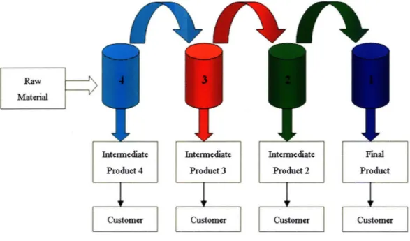
Many chemical or continuous production operations must manage multiple serial processes where the product from one stage is an input to the next stage. The

manufacturing stages also have some certain production reliability. This means that inventory is needed in each stage in case the upstream stage is down. The total costs in the production process are comprised of inventory holding costs and penalty costs when a

supply shortage occurs. Therefore, a good inventory policy is required to determine how much inventory to keep in each stage in order to minimize the total costs while meeting a specified certain Cycle Service Level (CSL).

Figure 1 is a typical four-echelon several production/inventory system in a chemical plant with variable supply, demand and production uncertainty.

Raw

Material

Figure 1: Four-echelon Production Process of a Chemical Plant

11(

Inventory is typically stocked at four tanks in a supply chain and the varieties of stock will include raw material, semi-finished products and finished products to distribute to different clients. As it is difficult to balance production and demand variability in the different stages of the supply chain, there is a need for managers who control all the products in multi-echelon network to have a simple and easy method to make daily plans.

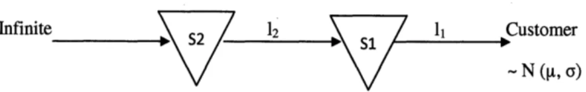
In order to simply the problem, in this thesis we will examine a two-echelon serial system as Figure 2. The stochastic demand, lead time and supply will be considered as variables and their impact will be studied.

Infinite .ustomer

- N ([t, (Y)

Figure 2: The Considered Two-echelon Serial Inventory System

In this system, we set the raw material from outside infinite and it flows to Stage 2 (S2) for the first production. Then product after S2 flows to Stage 1 (SI) as raw material

for the second production and the product after S1 is the final product for customer. The customer demand - N (u, a) obeys the normal distribution with mean g, standard

deviation a. We define 12 as Lead Time to supply Production 2 to Stage 1 and 11 as Lead Time to supply final production to customer.

Chapter 2 summarizes the current research on multi-echelon inventory policies. We discuss three important methodologies: Clark-Scarf (1960), Axsater (2006) and

Geert-Jan van Houtum (2004). We compare the limitations of application in multi-echelon production/inventory environment.

Following the Literature review, Chapter 3 describes the Geert-Jan van Houtum Methodology to be used for the simulation verification. This methodology closely examines two-echelon model and provides a modeling procedure, analysis, computation issues and further extensions. The second part briefly introduces some ideas about

simulation. As the simple closed form analytic solutions are not possible to solve this complex multi-echelon issue, a simulation is used to assess the situation and provide practical solutions which can be used for a company's daily operations.

Chapter 4 discusses the results of the simulation modeling. Four cases are simulated: 1) deterministic lead time, 2) stochastic lead time with normal delays, 3) stochastic lead time with longer delays, and 4) stochastic lead time with more frequent and shorter delays. The outcomes are analyzed and the insights which can be used by the company to determine the production/inventory policies are presented.

Finally, Chapter 5 summarizes what we have done in this research study including the general conclusions, highlights of the work and areas for research extensions.

Chapter 2 Base-stock Policy for Multi-echelon: Literature Review

The earliest module used for solving multi-echelon inventory is found in Clark-Scarf (1960) where they describe how to determine safety stocks in a serial multi-echelon inventory system. This method is exact for the serial systems and can be considered as a decomposition technique which decomposes the total costs into holding cost and penalty cost for each echelon.

Clark and Scarf start the research from a single installation model. After a sequence of purchasing decisions is made at the beginning of a number of regularly spaced intervals, the total costs in term of holding cost and shortage cost over the period is given by the following equation:

hx + p fx (t- x)4Q(t) dt; x > 0

L (x)

p f (t - x) Q(t) dt; x <= 0

where x: the stock unit on hand at the beginning of the period

h: unit holding cost

p: unit shortage cost

0(t): the demand function during the period 14

In the equation, hx refers to the holding cost for one echelon which is determined by unit holding cost and stock unit and the part p fx(t - x)Q(t) dt refers to the penalty cost which is unit shortage cost times by total shortage unit.

The following assumptions are made:

* Demand is only from the lowest installation (installation 1) -Customer in the system;

* The purchasing cost and shipping cost are linear and there is no setup cost. * A linear holding and shortage cost will be operative at the lowest installation

(installation 1).

* Each echelon backlogs excess demand.

In the model, their purpose is to find an optimal policy for an inventory problem with n periods remaining, which is the purchasing policy to minimize the total discounted cost. The minimizing value is the optimal purchase quantity for the given stock

configuration and they assume that all excess demand is backlogged until the necessary stock becomes available.

Then they turn attention to the multiple-installation model with finite time horizon and stochastic period demand. In the first step they consider the most downstream

installation which is facing the Customer demand, and the shortages at the next upstream installation cause stochastic delays. Of course, the stochastic delays will imply certain additional costs which are evaluated and added as shortage costs for determining an optimal policy for the next upstream installation.

Finally, Clark and Scarf conclude that the above expression is a convex function of x2, so that the optimal policy for the second echelon will be (S, s) policy, where S is

inventory stock of up-to- level, s is the safety stock. They also described how for more than two echelons, that is the same procedure can be followed.

Axsater (2006) used Clark-Scarf (1960) to study a simple two-echelon serial system which is based on 1) periodic review, 2) continuous period demand at echelon 1 is normally distributed and independent across periods, 3) demand that cannot be met

directly from stock is backordered, 4) supply to echelon 2 from outside is infinite, and 5) standard holding and backorder costs but no ordering or setup costs.

The purpose is to minimize the total expected holding and backorder costs per period. They consider the holding costs for stock on hand at the echelons. They do not include the expected holding costs for units in transportation from echelon 2 to echelon 1. These costs are not affected by the control policy.

Then they generalize the model to more than two echelons. The additional costs at echelon 2 due to insufficient supply are used as the shortage costs at echelon 3, etc. It is also easy to generalize to a batch-ordering policy at the most upstream echelon. For two echelons and normally distributed demand, the exact solution is relatively easy to obtain, but in a general case the computations can be very time consuming.

They also note that the Clark-Scarf approach can be used for assembly systems such as component assembly. In fact, Rosling (1989) has demonstrated that an assembly system can be replaced by an equivalent serial system when carrying out the

computations. Chen and Song (2001) generalized the Clark-Scarf model to demand processes where demands in different time periods may be correlated.

Based on Clark and Scarf's research, Geert-Jan van Houtum studied the serial, two-echelon system with linear inventory holding and backordering costs and with the

minimization of the average costs over an infinite horizon. Figure 3 shows the serial, two-echelon system:

Raw Intermediate Final

Material: product product

ca

h2 hi + h2, p

Figure 3: The Serial, Two-echelon Production/Inventory System

In the above system, they considered the raw material from outside is infinite and flows to Stage 2 (S2) for the first production. Then intermediate product after S2 flows to

Stage 1 (S) as raw material for the second production and the product after Si is the final product for customer. The customer demand in a given single period t is denoted by Drt. They also defined 12 as Lead Time to supply Production 2 to Stage 1 and 11 as Lead Time to supply final production to customer, and hi, h2 are unit holding cost in Stage 1 and Stage 2 respectively. To simplify the problem, they assumed that there is no penalty cost between S1 and S2 but a penalty cost due to demand shortage for customer. Therefore, the

intermediate product in Stage 2 shall only involve holding cost (unit cost h2) and final product in Stage 1 shall involve total holding cost (unit cost h,+ h2) and penalty cost (unit cost p).

They assume that the following events happen in each period in this sequence: * at each stage, an order is placed;

* the orders arrive; * demand occurs;

* inventory holding and penalty costs are assessed. The following term definitions are used in this methodology:

* Echelon: the chain under consideration is called the echelon. For example, Echelon 1 consists of stock point 1, Echelon 2 consists of stock point 2, stock point 1, and pipeline in between, etc.

* Echelon stock (echelon inventory level): all physical stock at a given stock

point plus all materials in transit to or on hand at any stock point downstream minus eventual backlogs at the most downstream stock point. Echelon stock

of echelon I is called echelon stock 1, and is the same as Installation stock 1. Echelon stock of echelon 2 is also called echelon stock 2.

* Echelon inventory position: the echelon stock at a stock point plus all

materials in transition to the stock point. If we assume that a stock point never orders more than what is available at the next upstream stock point, the

echelon inventory position is equal to the echelon stock plus all materials on order.

It is clear that the first two events occur at the beginning of the period, and sometimes the order of these two events could be interchanged; the last event takes place at the end of a period and the demand may happen anywhere in between.

If H1 is used as the set all possible ordering policies and G (n) as the average costs of ordering policy for all n c II, our problem to achieve optimality can be solved by minimizing the total costs function G (x). In other words, our objective is to find an ordering policy under which the average costs per period are minimized. Therefore, the total costs including holding costs and penalty costs at the end of the period under consideration are equal to:

h2(x2 - X1) + (hi + h2)Xl+ +

P X1

where xl: customer demand

x2: demand from Echelon 1

Also, x = max{ 0, x } and x = max{ 0, -x }= -min{ 0, x ),x E R.

So the total costs can be rewritten as following:

= h2(X2 - X1) + (hi + h2)Xl+ + p X1

= h2(X2 - X1) + (hi + h2)X1 + (p +

ha

= h2x2 + hlXl + (p + hi + h2) X1

-The item h2x2 is the holding costs attached to echelon 2 (also called echelon 2

costs), and hlxl + (p + hi + h2) x1 is the costs attached to echelon 1 (also called echelon

1 costs). The item hlxj is the holding costs attached to echelon 1 and (p + hi + h2) is the

shortage unit cost including penalty cost, holding costs in Echelon 1 and 2, and xf- is the shortage unit for customer demand.

In order to solve the problem, Clark and Scarf set a base-stock policy as the ordering (or replenishment) policy. A base-stock policy can be denoted by (yi, y2), where

yl, y2 E R refers to the desired order-up-to level for the echelon 1 & 2 inventory position. Therefore, the total costs for the policy (yi, y2) including holding costs and penalty costs at the end of the period are equal to:

G (yl, y2) = h2 (2 - (12+ 1) )

+ hi(yi - EB1 -(11 + 1).) + (p + hi + h2) EBo

where BI: the shortage units at stock point 1

Bo: the shortfall units for customer demand

In summary, Clark and Scarf (1960) studies a serial, multi-echelon inventory system with linear inventory holding and backordering costs. Firstly, they introduced the concept and defined some terms of echelon stocks. Then they derived the optimality of base stock policies and the derivation of the decomposition result in a dynamic

programming framework.

Axsater (2006) is based on Clark-Scarf (1960) and develops a computation method for optimal policy. The difference is that Clark-Scarf (1960) considers a finite time horizon while Axsater (2006) assumes an infinite horizon. However, the

computation solution provided by Axsater (2006) can be very complicated and time consuming, thus is not easy for business use.

In comparison, van Houtum (2004) which also is based on Clark-Scarf (1960) considers a serial, two-echelon system with a linear inventory holding and backordering costs over an infinite horizon. The analysis for the two-echelon case contains all essential elements and also the computation is relatively simple.

Chapter 3 Methodology, Modeling and Simulation

This chapter first presents the Van-Houtum Model which is close to our problem and relatively easy to compute, thus we use it to verify the simulation results. Then we introduce the concept of base-stock policies and how to obtain the results. In the final section, we generally describe the model, building procedure and how to carry out the simulation.

3.1 van-Houtum Model

As the production/inventory systems in a chemical plant can be considered as multi-echelon systems with linear inventory holding and backordering costs over an infinite horizon, we apply Van-Houtum's methodology and computation procedure to determine inventory placement. We start by describing a model for a simple, serial, two-echelon system as Figure 3 which was first introduced in Chapter 2.

Raw Intermediate Final

Material: _{product product}

h2 hi + h2, P

Figure 3: The Serial, Two-echelon Production/Inventory System

ol

We consider a supply chain with two stages and a single product produced to stock. We call the upstream stage Stage 2 and the downstream stage Stage 1 and both stages consist of a production step, a transportation step, or a network of those steps, with a stock point at the end of the stage. In order to simplify the problem, we assume that Stage 2 is fed with infinite raw material and produces an intermediate product which is stored in stock point 2; Stage 1 produces a final product which is stored in stock point 1. External demand only occurs for the final product from customer.

We consider the time horizon as infinitely long and the time is divided into

periods of equal length. The length of each period is assumed to be equal to 1 and the unit could be hour, day or week, etc. We first define the echelon inventory position of a stock point as its echelon stock plus all materials in transit to the stock point. For example, the echelon inventory in position 1 equals the echelon stock 1 plus transiting material to echelon 1, the echelon inventory in position 2 equals the echelon stock 2 plus transiting material to echelon 2.

The value of the product at Stage 1 is higher than Stage 2. From Chapter 2 we can understand that the total costs comprise with two parts: Echelon 2 attached total holding cost h2x2, Echelon 1 attached holding cost hlx1 plus penalty cost (p + h, + h2) x1.

3.2 Base-stock Policies Introduction

In order to solve the business problem, we should set a base-stock policy as the ordering (or replenishment) policy which can be easily understood and used by

1. If we denote (yi, Y2) as the inventory policy, where Yi, Y2 E R. yl is the desired inventory level for Echelon 1 and Y2 is the desired inventory level for Echelon 2.

2. Then we set G (yl, y2) as the function of the average costs for a base-stock policy (yi, y2). As we know from Chapter 2, the total costs includes holding costs in Echelon 1 & 2, and penalty cost in Echelon 1, which can be written as following:

G (yi, y2) = h2X2 + hlX1 + (p + hi + h2) X1"

where hi: unit holding cost in Echelon 1

h2: unit holding cost in Echelon 2

xj: demand from customer for Echelon 1

x2: demand from Echelon 1 for Echelon 2

p: unit penalty cost for Echelon 1

xli: shortage unit of customer demand

The first term h2x2 is the holding costs attached to echelon 2, and the second item hlxl is the holding costs attached to echelon 1 and (p + h, + h2) X1_ is the penalty cost when xl- is unfulfilled units for customer.

If the base stock policy (S1, S2) is the optimal base-stock levels at Echelon

G (S₁, S₂)= h₂S2+ hiS1+ (p + hi + h2) Sl

As the optimal policy which is the minimum cost function, (S1, S2) should

satisfy:

GI' (S1) =

gi

(SI)

=

0

G' (S1, S2) = g (S1, S2)= 0

3. We can use Newsboy characterizations to carry out the calculation and obtain the value of S1.

P

(Bo(') = 0

= (p

+

h

)

/

(p

+

hi+

h

)

Bo(I)= (Dto+₁2, t+12+1- S1)+

Bo01 is the shortfall for customer demand which is the demand during the lead time 11 minus S1. The probability of no shortfall can be calculated by Newsboy approach (p + h₂) / (p + hi+ h₂

)-4. Apply again Newsboy characterizations to calculate the optimal base-stock level S2 :

P Bo = 0) = p / (p + hi+ h2)

B₁ = (Dto, t0+12-1- (S2 -S1))+

Bo = (B₁ + Dt0+₁₂, t0+12+11- S1)+

(p + h2)/(p + hi+ h2). When determining S2, the full system is considered and the value

for S2 is equal to p / (p + hi+ h2).

In summary, we can follow the above procedure to obtain the basestock policy which is the optimal inventory policy for the serial, two-echelon inventory system basestock policy. In this methodology, we derive a decomposition result and present Newsboy characterizations to determine the optimal basestock levels.

3.3 Computation Procedure

Through the above methodology, we can obtain the optimal policy (SI, S2) and then

get the optimal total costs G (SI, S2) accordingly. However, there is a simpler

approximate procedure that is still accurate enough to use in business. As above

discussed, the optimal base-stock level Si follows the Newsboy characterization and can be determined by P (Bo0 1 = 0 ) = (p + h2) / (p + hji h2). For any Si the probability P

(Bo1 _{) ) = 0 could be approximated as following procedure:}

1. First determine the property of Customer demand: the mean = (11+ 1) [t; the standard deviation = (11+ 1)1/2a, and cy is the standard deviation of the demand distribution.

2. Find a suitable distribution configuration for Dt0+1₂,

tO+12+11-3. Determine P (Bo(') = 0) = P(Dtm+12, t+12+11 5 Si)

4. Next we will determine the optimal base-stock level S2. We can use the

Newsboy characterization to calculate by P( Bo = 0 ) = p / (p + hi+ h2).

When S2> Si, the probability P{ Bo = 0) may be approximated as following: 26

1. First we should determine the property of Customer demand. The mean =

12 I and the standard deviation = (12)1/20, and a is the standard deviation of the demand distribution.

2. Find a suitable distribution configuration for Dto, t0+12-1.

3. Determine the first two moments of B1.

4. Determine the first two moments of B1+ Dt0+12, t0+12+11. The mean = EB1 + (11+1) [, the standard deviation = (Var(B₁) + (11 + 1) 02)1/2, and a is the standard deviation of the demand distribution.

5. Find a suitable distribution configuration for Bi+ Dto+12, t0+12+11.

6. Determine P({ Bo = 0) = P B1+ Dto+12, t+12+11 S 1 .

3.4 Modeling and Simulation

In many cases, a process is so complex that it can't be solved by using some equation or simple methodology. So that building a model and running simulation is often used for achieving a solution.

A simulation is a computerized version of the model which is run over time to study the implications of the defined interactions. Simulation process is an iterative development: first develop a draft model, simulate it, learn from the simulation, then revise the model, and continue the iterations until the goal is achieved.

For our simulation of the multi-echelon inventory system, we will follow the below procedure to build and develop the model and carrying out case simulations accordingly:

1. Setting of Scope and Objectives: Find the base-stock policy to achieve the minimum cost at some certain Cycle Service Level (CSL);

2. Gathering of Data: As the model is a theoretical model which will be applied in broad production lines, we don't need the specific data from the company, just make some reasonable assumptions and use general data. 3. Building, Verifying and Validating the Model: According to the

production process, we build a model with Microsoft Excel, and then run an initial base case simulation. The results shall be verified using optimal approach based on Clark-Scarf Model. If we satisfy the verification, more case simulations will be run as sensitive analysis.

4. Output Analysis and Results: After all case simulations, we will compare with the results and carry out the sensitive analysis in order to see how each variable affects the outcome.

5. Conclusions and Direction of Future Work: Then we will get conclusions which will be used to establish a base-stock inventory policy. Finally, the future work shall be provided in order to improve the model.

3.5

Summary

This chapter discussed the methodology to be used for computing the base-stock policy to solve the problem faced by the company, and provided the computation procedure with details. Finally, this chapter presented the modeling and simulation procedure from how to set scope and objectives, gathering data, building and verifying

model, to analyze results and find conclusions and insights. Next, this heuristic method and procedure is applied to modeling and simulation to solve the problem.

Chapter 4 Model and Case Simulations

4.1

Modeling Procedure

Based on the initial data and information provided by the company, we start from a two-echelon model. In order to simplify the model, we first make some assumptions then create the model in Excel according to the company's inventory/manufacture line. Then the model is expanded with more variables and complication.

4.1.1 Two-echelon Model

The supply chain for the chemical plant is very complex system involving multi-echelon, multi-stage and multi-uncertainty problem, which also affect each other.

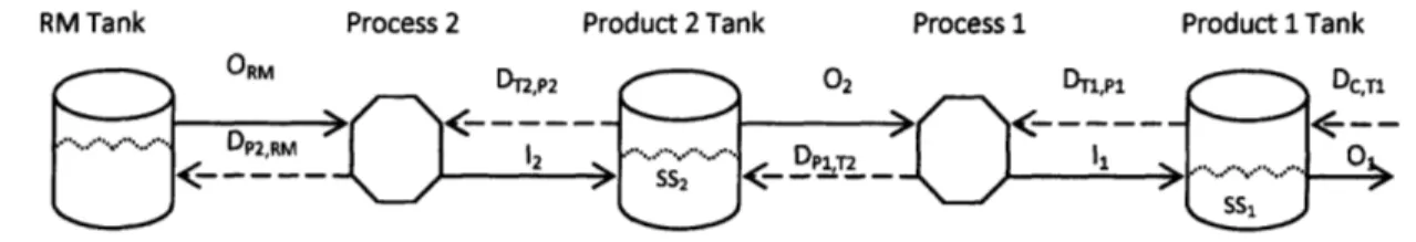
Therefore, we adopt a spiral approach by solving a simple model first then adding complexity. Starting from a simple model, we focus on two-echelon model as Figure 4:

Product 2 Tank Process 1 Product 1 Tank

Figure 4: Simplified Two-echelon Production Process

Raw Material Tank

Shipped Out Amount of Raw Material from RM Tank to Process 2

RM Tank Process 2

where RM Tank:

ORM:

DP2,RM: Raw Material Demand from Process 2

DT2,P2 : Product 2Demand from Product 2 Tank

12: Flowed In Amount of Product 2 from Process 2 to Product

2 Tank

SS2 : Safety Stock of Product 2 in Product 2 Tank

02 : Shipped Out Amount of Product 2 from Product 2 to Process 1

DTJ,p : Product 1Demand from Product 1 Tank

I ,: Flowed In Amount of Product 1 from Process 1 to Product 1 Tank

SS1 : Safety Stock of Product 1 in Product 1 Tank

O1 : Shipped Out Amount of Product 1 from Product 1 to Customer

DC, T : Product 1Demand from Customer

The following assumptions are made in this two-echelon stage:

* Demand for Product 2 from Echelon 1 flows into downstream production line as the raw material and the rest is kept in Tank 2 as safety stock inventory.

* There is no Customer demand existing for Product 2 and the only Customer demand is for Product 1 (end-product).

* For Product 1, if there is enough in Tank 1 the Customer demand will be fulfilled and the required amount will be transported to Customer and the rest is kept in Tank 1 as safety stock inventory. If there is not enough in Tank 1, the demand will be backordered and fulfilled in the future as soon as there is surplus left in Tank 1 after fulfilled Customer demand in that period.

During real production in this chemical plant, the most critical issue is the production reliability. From the information provided by a chemical plant, we note that the equipment reliability and the downtime duration for each echelon can be considered as identical in order to simplify the problem. Based upon the above assumptions, we took the following steps to build a model in Microsoft Excel:

1. We simulated 200 years operation at the daily level. The lead time variability was simulated via a Monte Carlo method. We also assume that the Lead time = 1 day if the production line runs well without downtime, therefore in our model the stochastic Lead time obeys the below distribution:

* Probability of no production downtime : 85% * Probability of production downtime 5 1 day: 90% * Probability of production downtime 5 2 day: 95% * Probability of production downtime 5 3 day: 100%

2. From the random simulation, we obtain the production lead time probability for each echelon then figure out the lead time date distribution. If one stage is down, there is no production at that stage, which means that the plant manager has to use the safety stock in the inventory tank as next stage's raw material or end-product for Customer.

3. For Product 1, if there is enough in Tank 1 the Customer demand will be fulfilled and the required amount will be transported to Customer and the rest is kept in

Tank 1 as safety stock inventory. If there is not enough in Tank 1, the demand will be backordered and fulfilled in the future as soon as there is surplus left in Tank 1 after fulfilled Customer demand in that period.

4. Raw material supply for Stage 2 is infinite.

5. Customer demand for Product 1 at Stage 1 obeys normal distribution - N (p., a), where pt is the average demand and a is the standard deviation. Based on this distribution, we randomly generate the demand by using Monte Carlo method with Microsoft Excel.

6. The inventory tank capacity is 5000t, thus in the model we assume a range from 500t to 5000t (100% full) as safety stock in inventory tank for each echelon, then combine the safety stocks for Echelon 1 and 2 to run the simulations. The results are CSL (cycle service level), FR (fill rate) and TC (total cost) for each inventory combination.

7. Finally, we will run one lead time deterministic case and three stochastic cases through which we can obtain insights and general guidelines for the company in order to manage the daily manufacture and operations.

In Stage 1, the demand for product 1 (DcT) will be shipped from product 1 tank to Customer. Dcra obeys Normal distribution with the mean of 1000 ton/day and standard deviation 100 tons. The coefficient of variable is 0.10.

* All unfilled Customer demands are backordered and will be fulfilled as long as there is surplus (after the Customer demand in that period has been fulfilled) in product 1 tank in the future.

* Product 1 is produced by process 1 and stored in product 1 tank. The supply of product 1 (SP1M₁) subject to both the production capability (S₁) and

equipment reliability of process 1. The production capability S1 is 1600 tons.

The equipment reliability obeys different distributions that will be specified below.

* We assume that the cost of product 1 equals US$15000/ton. The carrying cost is 0.2$/$/year. There are 365 days per year. So the holding cost of product 1 (hl) equals (15000$/ton*0.2$/$/year)/(365 days/year) = 8.22 $/ton/day. * Penalty cost of product 1 (Pl) equals 1000 $/ton/year or 2.74 $/ton/day.

In Stage 2:

* There is no Customer demand for product 2. The demand for product 2 (DP1T2)

only comes from downstream production (production 1) that uses product 2 as raw material.

* All unfilled demands are backordered and will be fulfilled as long as there is surplus (after the Customer demand in that period has been fulfilled) in product 2 tank in the future.

* Product 2 is produced by process 2 and stored in product 2 tank. It is subjected to both the production capability (S2) and equipment reliability of process 2.

The production capability S2 equals 1600 tons. The equipment reliability obeys different distributions that will be specified below.

* We assume that the cost of product 2 equals 10000 $/ton. The carrying cost is 0.2$/$/year. There are 365 days per year; the holding cost of product 2 equals (10000$/ton*0.2$/$/year)/(365 days/year) = 5.48 $/ton/day.

4.2 Simulations and Insights

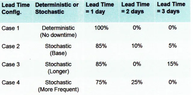
In order to find how each variable affects the base-stock policy, we run four sets of simulations as following:

* Case 1 (Deterministic Lead time): In this case, we assume that there is no equipment down time. This is the simplest case with deterministic lead time and the result can be verified by van Houtum method to ascertain the

correctness of the simulation. In this case, the lead-time for both echelons equals 1 day.

* Case 2 (Stochastic Lead time): in this case, we change the deterministic lead-time to stochastic lead-lead-time. The equipment reliability equals 85%. Of the remaining 15%, it will be down for 1 day in 10% of the total case and 2 days in 5% of the total case. As the lead-time is 1 day when there is no down time, the lead-time for both echelons obeys P{Lead Time < 1, 2, 31 = {85%, 95%,

100%}.

* Case3 (Stochastic Lead time): For Case 3, we keep the equipment reliability unchanged (85%) _{but prolong the equipment downtime to 2 days. i.e. of the} rest 15% of the downtime, it will always be down for 2 days. As the lead-time

is 1 day when there is no down time, the lead-time for both echelons obeys P{Lea Time < 1, 2, 3} = {85%, 85%, 100% }.

Case4 (Stochastic Lead time): Based on Case2, we reduce the equipment reliability to 75% but shorten the equipment downtime to 1 day. i.e. of the rest 25% of the total time, it will always be down for 1 day. As the lead-time is 1 day when there is no down time, the lead-time for both echelon obey P{ Lead Time < 1, 2, 3} = {75%, 100%, 100% }.

In summary, the characteristics of four cases as following:

Lead Time Deterministic or Lead Time

Lead Time

Lead Time

Config.

Stochastic

=I day

2

days

3

days

Case

1

Deterministic

100%

0%

0%

(No

downtime)

Case 2

Stochastic

85%

10%

5%

(Base)

Case 3

Stochastic

85%

0%

15%

(Longer)

Case 4

Stochastic

75%

25%

0%

(More Frequent)

Table 1: Four Simulation Cases

4.2.1 Overview of Notation

S2: Stage 2 order up to level

S: Total order up to level in Stage 1 & 2, S = S1 + S₂

hi: Inventory holding cost parameter for stage 1

h2: Inventory holding cost parameter for stage 2

p: Penalty cost parameter

1: Production lead-time if the equipment runs properly

E(D): Expectation of customer demand over lead-time 1

a: Standard deviation of customer demand over lead-time 1

MI: Moment 1, the specific Si higher than which the CSL/FR start to continuously increase.

M2: Moment 2, the specific Si higher than which the CSLIFR start to continuously decrease.

M3: Moment 3, the specific S1 higher than which the CSL/FR start to remain relatively stable.

4.2.2 Insights on Cycle Service Level

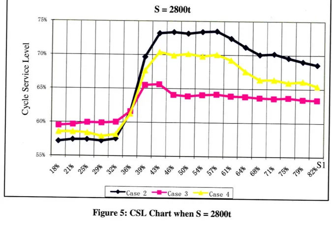
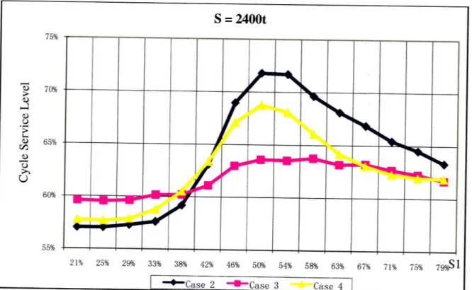
Below are Cycle Service Level (CSL) curves for Case 2 (base), Case 3 (longer) and Case 4 (more frequent) when S = 2800t, 2600t and 2400t:

Figure 5: CSL Chart when S = 2800t

Figure 6: CSL Chart when S = 2600t

S = 2800t

75%

Figure 7: CSL Chart when S = 2400t

4.2.2.1 How does the Distribution Configuration Affect CSL

As shown in figure 5, 6 _{and 7, we simulate with different lead-time distributions} and S levels, and in all three cases the service level starts a continuous, obvious increase when S1 is higher than 900. But when S1 is higher than 1200, the CSL will reach a relatively high level and keep very stable because there has been enough safety stock in stage 1 to cope with customer demand level and demand uncertainty already and higher S1 can't help to improve CSL too much.

In the last section, we defined M1 as the specific S1 higher than which CSL/FR start to continuously increase and M3 as the specific S, higher than which CSL/FR start

39 S = 2400t 75% 70% 65% 60% 55% 21% 25% 29% 33% 38% 42% 46% 50% 54% 58% 63% 67% 71% 75% ₇₉%S1

to remain relatively stable. So, here we can say that Ml = 900t and M3 = 1200t. As E(D) equals to 1000t and ( equals to 100t, we can tentatively assume that M1 = E(D) - F and M3 = E(D) + _{2c0. Then we change the demand level E(D) and demand uncertainty a to} test our conclusion.

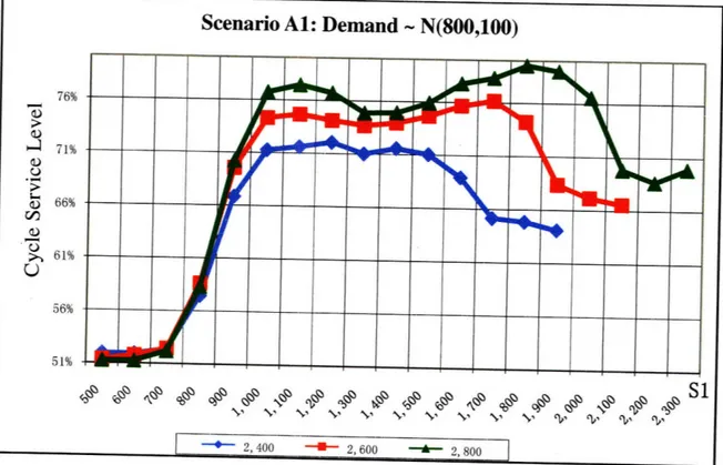
We use Case 2 as an example and change variable of the demand distribution to carry out the sensitive analysis:

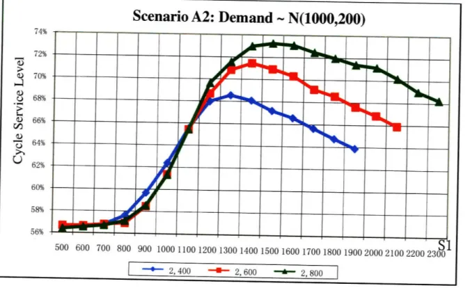
* _{Scenario Al - N(800,100): E(D) = 800t, a = 100t.} * Scenario A2 - _{N(1000,200): E(D) = 1000t, c = 200t.} * _{Scenario A3 - N(800,300): E(D) = 800t, a = 300t.}

For each scenario, we collect the simulation data and then put all three curves for S =2800t, 2600t and 2400t into one chart as shown below:

S = _{2400t, 2600t and 2800t for Scenario Al}

Scenario Al: Demand ~ N(800,100)

76% 0o 0) d)r - 61% 56% 51% S1 2, 600 ' 2, 800 I I *- 2,400

Figure 8: CSL Curves when ý-4

S0 e, If k,

Figure 9: CSL Curves when S = _{2400t, 2600t and 2800t for Scenario A2}

S2, 400 _{2, 600 A 2, 800}

Figure 10: CSL Curves when S = _{2400t, 2600t and 2800t for Scenario A3}

Scenario A2: Demand - N(1000,200)

74% 72% a 70% o 68% ) 66% S64% U 62% 60% 58% 56%

I -

1

Scenario A3: Demand ~ N(800,300)

66% O 61% U

From the above figures, we can find out that the M1 change to 700 (M1 = E(D) -a = 800 - 100), 800 (Ml = E(D) - a = 1000 -200) and 500 (Ml = E(D) - a = 800 -300), and M3 change to 1000 (M3 = E(D) + 2a = 800 + 200), 1400 (M3 = E(D) + 2c = 1000 + 400) and 1400 (M3 = E(D) + 2c = 800 + 600) respectively.

Using the same method, we can also find out the point that the CSL start to decrease: M2 = S - (E(D) + o).

So we can make the conclusion that given S, to achieve high CSL, we should at least ensure that Si is no less than E(D) + 2c and S2 is no less than E(D)+ c. If S is lower than the sum of E(D) -a and E(D) + c, raise S1 as high as possible.

4.2.2.2 How does the Production reliability Affect CSL

Then we study the change of lead-time distribution and its affection on CSL. Firstly we compare Case 3 (longer) with Case 2 (base), i.e. study its affection on CSL if the lead-time distribution is changed from the base case (Case 2) lead time distribution P{LT = 1, 2, 3) = {85%, 10%, 5%) to longer downtime (Case 3) lead time distribution P{LT = 1,2,3) = {85%, 0%, 15% }, i.e. the equipment reliability keeps unchanged but if the equipment is down, it will need more time to be recovered.

The average lead-time increases from 1.2 days (85%*1+10%*2+5%*3=1.2) to 1.3 days (85%*1+0%*2+15%*3=1.3) or by 8.3%. The minimum and maximum service level in Case 2 is 56.88% and 73.51%. The maximum is 29% higher than the minimum. The minimum and maximum of service level in Case 3 is 59.47% and 65.63%. The maximum CSL is only 10% higher than the minimum one. We can find out that if down time is long, the distribution configuration does not affect CSL too much.

Secondly, we compare Case 4 (more frequent) with Case 2 (base), i.e. study its affection on CSL if the lead-time distribution is changed from the base case (Case 2) lead time distribution P{LT = 1, 2, 3) = {85%, 10%, 5% } to more frequent but shorter

downtime (Case 4) lead time distribution P{LT = 1, 2, 3) = {75%,25%,0% }, i.e. the equipment reliability is lower but it can be recovered soon.

The average lead-time increases from 1.2 days (85%*1 +10%*2+5%*3=1.2) to 1.25 days (75%*1+25%*2+0%*3=1.25) or about 4.2%. The minimum and maximum of service level in Case 2 is 56.88% and 73.51%. The maximum is 29% higher than the minimum one. The minimum and maximum of service level in Case 4 is 57.6% and 70.37%. The maximum is 22% larger than the minimum one. We can see that if lead-time is short, different distribution configuration of S will affect CSL dramatically.

We also build another scenario which is called scenario A4 to verify this insight: we change the lead-time distribution from P{LT = 1, 2, 3) = {85%, 10%, 5%) to P{LT = 1, 2, 3) = { 50%, 50%, 0%) and reduce the E(D) from 1000t to 600t. The average lead-time increases from 1.2 days (85%*1+10%*2+5%*3=1.2) to 1.5 days

Figure 11: CSL Curves when S = _{2400t, 2600t and 2800t for Scenario A4}

The minimum and maximum of service level in case 2 are 56.88% and 73.51%. The maximum is 29% higher than the minimum one. The minimum and maximum

service level in scenario A4 is 49.35% and 88.44%. The maximum is 79% higher than the minimum one.

So we can conclude that allocating S following the principles mentioned in previous section is particularly important in a production process with short but relatively frequent downtime, which is the current situation our sponsor company faced.

4.2.3 Insights on Fill Rate

Scenario A4: Demand ~N(600, 100),

P{LT=1,2,3}={50 % ,50% ,0% }

Below are Fill Rate (FR) charts for Case 2 (base), Case 3 (longer) and Case 4 (more frequent) when S = 2800t, 2600t and 2400t:

Figure 12: Fill Rate (FR) Curves when S = 2800t

S = 2600t 80% 78% -. 76% 74% S72% 70% 68% 66% 64% 19% 23% 27% 31% 35% 38% 42% 46% 50% 54% 58% 62% 65% 69% 73% 77% 81V

- Case 2 Case 3 Case 4

Figure 13: Fill Rate (FR) Curves when S = 2600t

S = 2800t 80% 78% 76% 74% eh 72% _ 70% 68% 66% 64%

S = 2400t

Figure 14: Fill Rate (FR) curves when S = 2400t

From the figures above, we can find out that the curves in Case 2 and Case 4 have almost the same trend except the average fill rate of Case 4 is slightly lower than that of Case 2, which is caused by the lead-time distribution. So here we analyze Case 2 and Case 4 together and then move on to Case 3.

4.2.3.1 Two moments with Shorter Downtime (Case 2 and Case 4)

From figure 12, 13 and 14 we can see that FR will keep a relatively high level if we can guarantee both S1 and S2 higher than 1100t. As long as this minimum requirement

satisfied, different distribution configurations of S will not affect the FR too much. But if S1 or S2 is lower than 1100t, the FR will decrease obviously with the decrease of S1 or S

2.

After some simulations we also find out that this key point is always slightly higher than 46 80% 78% 76% 74% 72% 70% 68% 66% 64% 67% 71% 75% 7991 21% 25% 29% 33% 38% 42% 46% 50% 54% 58% 63%

I

E(D), a or different lead-time distribution does not affect this insight. Below are the results of the simulations with different lead-time distribution, E(D) and Y and followed with our analysis.

We use Case 2 as an example and change variable of the demand distribution to carry out the sensitive analysis:

* Scenario B1 ~ N(800, 100): E(D) = 800t, c = 100t. * Scenario B2 - _{N(1000, 100): E(D) = 1000t, T = 100t.} * Scenario B3 - N(1000, 200): E(D) = 1000t, T = 200t.

* Scenario B4: we change the lead-time distribution from P{ LT = 1, 2, 31 = {85%, 10%, 5%} to P{LT = 1, 2, 3} = {75%, 25%, 0%} .

For each scenario, we collect the simulation data and then put all three curves for S=2800t, 2600t and 2400t into one chart as shown below:

500 600 700 800 900

1000

1100 1200

1300 1400

_{1500 1600 1700 1800 1900 2000 2100 2200}

2301

* 2, 400 - 2,600 2, 800

Figure 15: FR Curves when S = _{2400t, 2600t and 2800t for Scenario B1}

47

-- 2, 400 - 2, 600 2, 800

Figure 16: FR Curves when S = 2400t, 2600t and 2800t for Scenario B2

1

Figure 17: FR Curves when S = _{2400t, 2600t and 2800t for Scenario B3}

Scenario B2: Demand-N(1100,100) 84% 82% 80% 78% 76% 74% 72% 70% Scenario B3: Demand-N(1000,200) 84% 82%

a

#z#zp#####S# #s

I

Scenario B4: P{LT=1,2,3}={75%,25%,0% }

Figure 18: FR Curves when S = 2400t, 2600t and 2800t for Scenario B4

We can conclude that when the downtime is relatively short, to achieve high FR, we should at least guarantee both S1 and S2 higher than E(D). As long as this requirement satisfied, different distribution configurations of S will not affect the FR too much. But if S1 or S2 is lower than that the minimum requirement, the FR will decrease obviously with the decrease of S1 or S2.

4.2.3.2 Turning Point in cases with Longer Downtime (Case 3)

From case 3 we can see that FR decreases with the increase of S1 with given S. But there is an abrupt decrease in FR when S2 is less than 1700t. We will try to find out

what factors cause this.

84% 82% 80% 78% 76% 74% 72% 70% 68% 66% 2000 2100 2200 2300 500 600 700 800 900 1000 1100 1200 1300 1400 1500 1600 1700 1800 1900

1

--- 2,400

- 2,600

--

2,800

I

Firstly we see whether the demand will affect. We change the demand from -N(l000,100) to -N(800,100). We call this scenario B5 and the chart is as below:

I - 2, 400 - 2,600 2, 800

Figure 19: FR Curves when S = _{2400t, 2600t and 2800t for Scenario B5}

We can see that there is still an abrupt decrease in FR when S2 is less than 1700t. So it is not caused by demand. Then we change the G _{to see whether it is the root cause.}

We base on scenario B5 and change a from 100t to 200t to get scenario B6. There is a similar abrupt decrease. The chart is shown below:

Scenario B6: Demand-N(800,200)

Figure 20: FR Curves when S = _{2400t, 2600t and 2800t for Scenario B6}

The FR still abruptly decreases at 1700t and c is still not the root cause. After some simulations we suspect that maybe it is caused by the restriction on productive capacity. We change the capacity from 1600 to 2000 and run the simulation again. The result confirmed our suspicion.

The chart is as below. We call it scenario B7.

500 600 700 800 900 1000 1100 1200 1300 1400 1500 1600 1700 1800 1900 2000 2100 2200 23Al

- 2, 600 2, 800

Scenario B7: capability =2000

Figure 21: FR Curves when S = _{2400t, 2600t and 2800t for Scenario B7}

From chart above and other charts in this section, we can conclude that FR decreases with the increase of Si with given S. So when the downtime is relatively long, we will always prefer to keep a high S2.

4.2.4 Insights on Total Cost

Below are Total Cost (TC) curves for Case 2 (base), Case 3 (longer) and Case 4 (more frequent) when S = 2800t, 2600t and 2400t:

66% 64% 62% 60% S58% 56% 54% 52% 50% 48% ,sl ?N C\ 'b s1 -- 2, 400 --- 2,600 2,800

S = 2800t 7, UU0 6,000 O S5,000 4, 000 3, 000 2. 000 4I4 -q K-+--i--" i I I i I I I 18% _{21% 25% 29% 32% 36% 39% 43% 46% 50% 54% 57% 61% 64% 68% 71% 75% 79% 82%}

1 Case 2 U Case 3 Case 4

Figure 22: _{Total Cost (TC) Curves when S = 2800t}

Figure 23: _{Total Cost (TC) Curves when S = 2600t}

Umoo OW

F

4Lr

f

---I

IAJ

- L

c·4

--Z

van

weft

SAM'

S = 2400t

Figure 24: Total Cost (TC) Curves when S = 2400t

The total costs include penalty cost and holding cost. Holding cost = S1*hl +

S2*h2. Because hi is higher than h₂, the holding cost will increase with the increasing

percentage of S_{1. So if the reduced penalty cost brought by incremental safety stock in} Stage 1 cannot offset the incremental holding cost, we will prefer keep less in Stage 1. On the contrary, if more safety stock in Stage 1 can save penalty cost that is higher than the incremental holding cost, we will prefer keep more in Stage 1.

As we defined, Ml refers to the safety stock in Stage 1 after which the CSL/FR starts to increase. M2 refers to the safety stock in Stage 1 after which the CSLUFR starts to decrease. So the point with the lowest cost must between M1 and M2. We call this point a "sweet spot". At sweet spot (hi-h2)*x = p*y*E(D) or y/x = (h₁-h₂) / [p*E(D)]. (x is incremental of SI, y is increment of FR)

8, 000 7, 000 0 U 6,000 5,000 4, 000 3, 000 2. 000 67% 71% 75% 79981 21% 25% 29% 33% 38% 42% 46% 50% 54% 58% 63%

Then we'll see how to find out the sweet spot. According to the formula, it depends on the holding cost of Stage 1 (hi), holding cost of Stage 2 (h2), penalty cost (p) and increment of FR (y). In production, we can get hi, h2 and p easily. The only problem is how to get y. We have already provided some principles in previous sections.

But sometimes the calculation result of the point with lowest cost is slightly different from the simulation result. This is because our step in the simulation is not small enough (100 each step in our simulations), and also there are many random numbers in our simulations that bring some uncertainty.

As we can see from above charts and our analysis, the point with the lowest cost always appears between Ml and M2. And if comparing the three charts in this section we can also see that more safety stock does not guarantee lowest cost necessarily. If the saving on penalty cost cannot offset the incremental holding cost, the total cost will be even higher.

4.2.5 Insight and Instruction

Summarizing analysis above, we can have some insight and preliminary quantitative instructions for our sponsor company.

1. _{If the objective is to achieve high CSL, the company should ensure S1} higher than E(D) + 2_{0 and S}

2 higher than E(D) + a. If there is a constraint on S,

company should at least guarantee S1 higher than E(D) - a or as high as possible. So generally speaking, company should place more stock in stage 1 (closer to customer) to achieve high CSL. This principle is particularly important in a production process with short but relatively frequent downtime.

2. If the company wants to achieve high FR, it should follow different principles based on different lead-time distributions. When the downtime is relatively short, the company should at least guarantee both S1 and S2 higher than

E(D). As long as this requirement satisfied, different distribution configurations of S will not affect the fill rate too much so the only way is to increase S if the

company want to achieve higher FR. When the downtime is relatively long, we will always prefer to keep a high S2, i.e. the point of the uncertainty.

3. The point with the lowest cost always appears between Ml and M2. So if the company wants to find out this point, it can firstly determine several S

considering company strategy, tank capacity etc. and then narrow down the scope to from Ml to M2. Then we can do the simulations only for the points in that scope to find out the point with the lowest point.

4.3

Verification by van Houtum's Methodology

In order to verify the above simulation, we use Van Houtum Methodology to check whether our simulation results are accurate. First, we consider Scenario-i whose inputs as following:

* Supply from Echelon 2 to Echelon 1 = 1300 ton/day. * Customer demand for Echelon 1 = 1000 ton/day. * No Customer demand for Echelon 2.

We calculate the Cycle Service Level (CSL) based on different inventory combination in Echelon 1 (Si) and Echelon (S2). The outcomes as following:

Table 2: Computation result of Cycle Service Level (CSL)

The red-highlighted data mean that Cycle Service Level (CSL) under those inventory combinations in Echelon 2 and Echelon 1 is below the average. The green-highlighted ones mean that CSL under those inventory combinations is above the average.

From the results, in general we can say that CSL increases with the inventory level going up. It is clear that below 3000t CSL increases dramatically with the inventory level going up, but when inventory level beyond 3000t, CSL becomes much flat. That means when CSL reaches a certain point, it will be more difficult or need much more efforts to increase CSL comparing with below that certain point.

For Scenario-2, the condition is:

* Supply from Echelon 2 to Echelon 1 = 1200 ton/day. * Customer demand for Echelon 1 = 1000 ton/day. * No Customer demand for Echelon 2.

Then we input above data to run the simulation, the results are:

57 S O1 000t 2000t 3000t 4000t 5000t

1000t

2000t

-

i

3000t

4000t

U

i

iM

5000t•

Ui

Table 3: Computation result of Cycle Service Level (CSL)

As stated in Scenario-1, the red-highlighted data mean that Cycle Service Level

(CSL) is below the average; the ones green-highlighted mean that CSL under those

inventory combinations are above the average.

In general, CSL increases with the inventory level going up, but the point moves forward to 2500t. S 1000t 2000t 3000t 4000t 5000t

1000t

~

i

2000t

-

-

-

i

3000t

l

-

i

4000t

l

-

i

i

5000t

a

-

i

i

Chapter 5 Review and Conclusions

Here we will summarize the work done in this thesis: 1) the summary of the work we have done including problem identification, literature review, and modeling and case

simulations, 2) the highlights of some significant characteristics of this work, 3) Future work.

5.1

Summary of Work

In this thesis, we first introduce the problem which is experienced by many production companies with multi-echelon process line: how to manage this

production/inventory system involved some variable? Especially, in business companies need a simple method which is easy to understand and apply during manufacture and operation. Then we start to review the previous literature research on the multi-echelon

subject.

As the production/inventory systems in the chemical plant which we are working for can be considered as multi-echelon systems with linear inventory holding and

backordering costs over an infinite horizon, we apply Houtum's methodology and algorithm to figure out the base-stock inventory policy.

There are four variables involved in the process 1) supply including external and internal, 2) customer demand, 3) lead time and 4) production reliability. There are all varying along time (day, week or month). Therefore, we need to make simulations in order to closely examine the real situation. Four simulation cases are completed considering different variable combinations:

1) Case 1 (Deterministic): {LT=1, 2, 3 day(s)) = (100%, 0%, 0%}, 2) Case 2 (Base): {LT=1, 2, 3 day(s)) = {85%, 10%, 5%},

3) Case 3 (Longer): {LT=1, 2, 3 day(s) } = {85%, 0%, 15% },

4) Case 4 (More Frequent): {LT=1, 2, 3 day(s)) = (75%, 25%, 0%}.

Next we verify the simulation results to check whether the simulations are correct. Finally, Section 5.3 presents the insights and the conclusions which can be used by the company to determine the production/inventory policies.

5.2

Highlights of the Work

After the above research on the multi-echelon production/inventory process, we think that the following contributions are significant to be highlighted for the company and the industries:

* This thesis presents a typical solution to solve the real problem faced by industries, which is simulation the actual situation as near as possible and then verify the outcomes by recognized methodology.

* We first identify the problem and find four variable to be discussed and figure out their affect on the problem individually, through which we could obtain the insights and provide recommendations to the company accordingly.

* A simplified computation spreadsheet based on Excel is developed for the company and its supply chain team can use it to manage the production line in order to achieve the optimal inventory/production policy.

5.3

Recommendations for Future Work

As the limited time and resources, some work still has not been done in our nine-month research thesis. Hereby we give some recommendations for the future work:

* Add customer demands for intermediate product and attempt to figure out the product distribution configuration: how much sell to demanded customers, how much keep in tank as inventory and how much flow to next echelon for process. * Run more simulation cases to find the insights on the production rate, inventory

tank capacity, and additional value after downstream process, etc.

* Expand the heuristic procedure from two-echelon to three-echelon and four-echelon.

Reference List

Axsater, Sven, Inventory Control, 2nd Edition (2006 by Springer Science + Business Media, LLC).

Ahr, D. (2004). Operations research proceedings 2003.Selected papers of the

international conference on operations research (OR 2003), heidleberg, September 3-5,

2003. (Berlin; New York: Springer.)

Clark, A.J., An Informal Survey of Multi-echelon Inventory Theory, (Naval Research Logistics Quarterly, 1972).

Gershwin, S. B., Analysis and modeling of manufacturing systems, (Kluwer Academic Publishers, 60, 429, 2003)

Glasserman, Paul & Tayur, Sridhar, Sensitivity Analysis for Base-stock Levels in Multiechelon, (Management Science, Vol. 41, No. 2, (Feb., 1995), pp. 263-281, 1995)

Graves, S. C., A multi-echelon inventory model with fixed reorder intervals, Working Paper (Cambridge, Massachusetts Institute of Technology, 1989).

Graves, S. C. & Willems, Sean P., Optimizing Strategic Safety Stock Placement in Supply Chains, (Manufacturing & Service Operations Management, Vol. 2, No. 1, pp. 68-83,

2000)

Hiller, Federick S., Lieberman, Gerald J., Introduction to Operations Research, 6th ed. (McGraw-Hill, 1995)

Kok, A.G. de and Graves, S.C., Handbooks in OR & MS, Vol. 11, Chapter 3 Supply

Chain Design: Safety Stock Placement and Supply Chain Configuration.

Minner, S. Strategic safety stocks in supply chains. (Berlin; New York: Springer, 2000). Navia y de la Campa,Juan Marcelo Felipe, A continuous process for the manufacture of

caramels, (1951)

Ronald H. Ballou, Business Logistics Management: Planning, Organizing, and

Controlling, the Supply Chain, 4th ed. (Upper Saddle River, New Jersey: Prentice-Hall,

1998)

Schultz, S. J., Multi-echelon inventory control, MS Thesis (Cambridge, Massachusetts Institute of Technology, 1980).