HAL Id: insu-02395723
https://hal-insu.archives-ouvertes.fr/insu-02395723
Submitted on 11 Dec 2019
HAL is a multi-disciplinary open access
archive for the deposit and dissemination of sci-entific research documents, whether they are pub-lished or not. The documents may come from teaching and research institutions in France or abroad, or from public or private research centers.
L’archive ouverte pluridisciplinaire HAL, est destinée au dépôt et à la diffusion de documents scientifiques de niveau recherche, publiés ou non, émanant des établissements d’enseignement et de recherche français ou étrangers, des laboratoires publics ou privés.
Heterogeneous behaviour of unconfined Chalk aquifers
infer from combination of groundwater residence time,
hydrochemistry and hydrodynamic tools
Feifei Cao, Jessy Jaunat, Virginie Vergnaud-Ayraud, Nicolas Devau, Thierry
Labasque, Aurélie Guillou, Alexandra Guillaneuf, Julien Hubert, Luc
Aquilina, Patrick Ollivier
To cite this version:
Feifei Cao, Jessy Jaunat, Virginie Vergnaud-Ayraud, Nicolas Devau, Thierry Labasque, et al.. Het-erogeneous behaviour of unconfined Chalk aquifers infer from combination of groundwater residence time, hydrochemistry and hydrodynamic tools. Journal of Hydrology, Elsevier, 2020, 581, pp.124433. �10.1016/j.jhydrol.2019.124433�. �insu-02395723�
Journal Pre-proofs
Research papersHeterogeneous behaviour of unconfined Chalk aquifers infer from combination of groundwater residence time, hydrochemistry and hydrodynamic tools Feifei Cao, Jessy Jaunat, Virginie Vergnaud-Ayraud, Nicolas Devau, Thierry Labasque, Aurélie Guillou, Alexandra Guillaneuf, Julien Hubert, Luc Aquilina, Patrick Ollivier
PII: S0022-1694(19)31168-0
DOI: https://doi.org/10.1016/j.jhydrol.2019.124433
Reference: HYDROL 124433
To appear in: Journal of Hydrology
Received Date: 26 September 2019
Revised Date: 2 December 2019
Accepted Date: 3 December 2019
Please cite this article as: Cao, F., Jaunat, J., Vergnaud-Ayraud, V., Devau, N., Labasque, T., Guillou, A., Guillaneuf, A., Hubert, J., Aquilina, L., Ollivier, P., Heterogeneous behaviour of unconfined Chalk aquifers infer from combination of groundwater residence time, hydrochemistry and hydrodynamic tools, Journal of Hydrology (2019), doi: https://doi.org/10.1016/j.jhydrol.2019.124433
This is a PDF file of an article that has undergone enhancements after acceptance, such as the addition of a cover page and metadata, and formatting for readability, but it is not yet the definitive version of record. This version will undergo additional copyediting, typesetting and review before it is published in its final form, but we are providing this version to give early visibility of the article. Please note that, during the production process, errors may be discovered which could affect the content, and all legal disclaimers that apply to the journal pertain.
Heterogeneous behaviour of unconfined Chalk aquifers infer from
combination of groundwater residence time, hydrochemistry and
hydrodynamic tools
Feifei CAO (1), Jessy JAUNAT (1), Virginie VERGNAUD-AYRAUD (2), Nicolas DEVAU (3), Thierry
LABASQUE (2), Aurélie GUILLOU (2), Alexandra GUILLANEUF (1), Julien HUBERT (1), Luc
AQUILINA (2), Patrick OLLIVIER (3)
(1)Université de Reims Champagne-Ardenne – GEGENAA – EA 3795, 2 esplanade Roland Garros,
51100 Reims, France
(2)OSUR, Géosciences Rennes, UMR 6118, CNRS/Université Rennes-1, F-35042 Rennes, France (3)BRGM, 3 av. C. Guillemin, BP 36009, 45060 Orléans Cedex 2, France
*Corresponding author: Feifei CAO E-mail address: [email protected]
Abstract
Chalk groundwater is an important aquifer resource. It is intensively exploited for human use, with a large proportion utilized for drinking water. The improvement of the knowledge on Chalk aquifer hydrogeological functioning is essential for the management of this resource. Here, we developed a methodology based on a combination of hydrodynamic, hydrochemistry and groundwater dating tools. A study site with Chalk outcrops was selected in NE France where groundwater geochemistry and water level were monitored continuously for 2 years from 2017 to 2019 and groundwater residence time was estimated using CFCs and SF6. Overall, the aquifer has an inertial behaviour with respect to
recharge. Nevertheless, a rapid water level response following rainfall events was observed at one site, suggesting the presence of highly developed fracture network at the local scale. According to the mixing process (piston flow, exponential or binary mixing) defined at each sampling site, groundwater dating indicated rather heterogeneous ages ranging from modern to about 50 years. High spatial and temporal heterogeneities were observed and interpreted by a combination of hydrogeological setting, residence time and land use information, highlighting main factors governing the Chalk groundwater geochemistry including water level fluctuation, thickness of the Unsaturated Zone (UZ), superficial formations, distribution of fracture network, aquifer-river relations and human activities. A conceptual
model was proposed accordingly to explain the hydrogeological functioning of unconfined Chalk aquifers.
Highlights
Piezometry of unconfined Chalk aquifer shows mostly an inertial behaviour Groundwater residence times are various ranging from modern to about 50 years Factors governing heterogeneity of the Chalk groundwater geochemistry are evidenced Chalk groundwater geochemistry allows to assess the functioning of the water table
Keywords:
Chalk aquifer; Groundwater age; Water level; Geochemistry variability; Water resource; Unsaturated zone1 Introduction
The Chalk formation is widespread in northwestern Europe covering large areas between the Paris Basin, the London Basin, Denmark and the North West of Germany (Bakalowicz, 2018). Groundwater of the Chalk Aquifer is intensively exploited for human use, making it one of the most important aquifers over much of Northern Europe. In France, the Chalk aquifer covers about 20 % of the metropolitan territory with a total area of 110 000 km2 (Crampon et al., 1996; Roux, 2018) and
provides approximately 12 billion m3·year-1 of water, which accounts for 70% of the drinking water
consumed in the north of France (Lallahem, 2002). However, in recent decades, there is a growing evidence of the deterioration of the European Chalk groundwater quality due to human activities (Baran et al., 2008; Barhoum, 2014; Chen et al., 2019; Hakoun et al., 2017; Johnson et al., 2001; Longstaff et al., 1992). Aquifer protection requires a sound knowledge of the Chalk hydrogeology and groundwater geochemistry.
Fitzpatrick, 2011; Van den Daele et al., 2007). Fracture distribution in the Chalk is highly heterogeneous. Vertically, fractures are generally only developed towards the top of the aquifer (Allen et al., 1997). Laterally, fractures are more developed in river valleys than on interfluves as the structural weaknesses followed by valleys are more fractured and erosion along valleys favors the opening of horizontal fractures (Allen et al., 1997; Price, 1987; Price et al., 1993).
Recharge through the UZ can occur very rapidly through fractures or slowly within the matrix (Allen et al., 1997). Most studies consider that in the UZ, recharge is predominately through the Chalk matrix with a mean downward rate of about 1 m·year-1 (Barraclough et al., 1994; Brouyère et al., 2004; Chen
et al., 2019; Haria et al., 2003; Vachier et al., 1987; Van den Daele et al., 2007; Wellings, 1984). Recharge through fractures is faster but smaller in volume. It occurs episodically when the infiltration rate exceeds the hydraulic conductivity of the matrix (Ireson and Butler, 2011; Mathias et al., 2006; Price et al., 2000). Rapid flow could also temporally or locally be dominant, especially in zones where karstic systems are developed (Ireson et al., 2006; Mathias et al., 2006; Maurice, 2009). Flow rates have been estimated with values ranging from 1 to 20 km·day-1 in karstic systems and up to 1m·h-1 in
fissures (Allshorn et al., 2007; Baran et al., 2008; Calba, 1980; Devos et al., 2006; Ireson et al., 2006; Katz et al., 2009; MacDonald et al., 1998). It should be noted that karst flow has usually a small contribution to the recharge of Chalk aquifer but can cause punctual problems on groundwater quality such as nitrate and bacterial contaminations (Barhoum, 2014).
Chemical composition of the Chalk groundwater is mainly controlled by water-rock interactions due to the dissolution of primary rock minerals and the precipitation of second phases (Gillon et al., 2010). Most of the chemical characteristics of Chalk groundwater are acquired during initial percolation through the soil and upper Saturated Zone (SZ). As the Chalk matrix is dominated by carbonate minerals, a fast homogeneity of the baseline geochemistry is expected (Edmunds et al., 1987). However, spatial and temporal heterogeneities of the groundwater chemistry can be observed due to internal and external factors such as local variations of the rock mineralogy (e.g., presence of dolomitic bodies, clay-rich, phosphatic layers; Deconinck et al., 2005; Jarvis, 1980; Richard et al., 2005), the incongruent dissolution of Chalk and dolomitic impurities (Aquilina et al., 2003; Edmunds
et al., 1987; Gillon et al., 2010; Kloppmann et al., 1998), pollution caused by human activities (e.g., NO3-, Cl-, atrazine), especially agricultural application of fertilizer and pesticide (Barhoum, 2014;
Kloppmann et al., 1994) and the mixing between waters of different residence times and origins including rapidly percolated water, fissure water and matrix pore water (Gillon et al. 2010). The mixing process depends on water level fluctuation (Brouyère et al., 2004; Hakoun et al., 2017), structure of the superficial formation (Barhoum et al., 2014; El Janyani et al., 2014; Valdes et al., 2014), climate conditions and topography.
A better understanding of the mixing process and flow mechanisms within aquifers could be achieved by groundwater dating using natural or anthropogenic age tracers (Cook et al., 1995; Darling et al., 2012a; Jaunat et al., 2012; Santoni et al., 2016; Suckow, 2014). In case of young groundwater with residence times ranging from 0 to 60 years, atmospheric trace gases such as CFCs (chlorofluorocarbons) and SF6 (sulphur hexafluoride) could be used (e.g., Aeschbach‐Hertig et al.,
1999; Busenberg and Plummer, 1992; Cook and Solomon, 1995; Dunkle et al., 1993; Plummer et al., 2001; Vergnaud-Ayraud et al., 2008). An average age and a distribution of residence times of groundwater can be estimated considering various mixing models (the most commonly used are the piston flow, the binary or exponential mixing), providing information on aquifer functioning (Appelo and Postma, 2004; Cook et al., 2005; Małoszewski and Zuber, 1982). To date, only a few studies have been undertaken using CFCs and/or SF6 to understand groundwater flow in Chalk aquifers (Cary et al.,
2014; Darling et al., 2012b, 2005; Gooddy et al., 2006). Furthermore, no studies have combined geological characterization, hydrodynamic conditions (water level fluctuations and recharge process), residence time determination and groundwater geochemistry within a Chalk aquifer. A methodology that combines these different approaches could provide a comprehensive understanding of the Chalk aquifer functioning.
groundwater flow paths, mixings and geochemistry for a better understanding of the hydrogeological functioning of the aquifer.
2 Materials and methods
2.1 Site description
The study area is located at the East of the city of Reims in the Champagne region (NE of France; Figure 1) and covers approximately 500 km2 between the Suippe River (as the northern and western
boundary) and the Vesle River (as the southern boundary). Both the two rivers have several tributaries; the Prosne River (tributary of the Vesle River) is dry for most of the time while others are permanent watercourses (Figure 1).
The Cretaceous formations outcropping on the surface of the study area are constituted by: Coniacian (C3), Santonian (C4) and Campanian (C5) Chalks (Figure 1). Despite the different age of formation, the three Chalks present a similar lithology. The first 10 – 20 meters of the Champagne Chalk are significantly fractured and the fracturing decreases with depth (Mangeret et al., 2012; Vachier et al., 1987). The Chalk formation is partially covered by Tertiary formations (10 – 50 m; Laurain et al., 1981) at the Berru Mount and by Quaternary formations including graveluche, colluvium and alluvium (Figure 1). Graveluche (also called grèze) refers to a periglacial formation with a maximum thickness of 6 to 10 meters (Rouxel-David et al., 2002b). During the Quaternary, the long period of freeze - thaw alternation produced movement in the terrain. Graveluches, resulting from this gelification process of the chalk, are very variable in particle size and composition with more or less content on clay and silt (Vernhet, 2007). The graveluche formation is more widely spread in the north (the catchment area of the Suippe River) than in the south of the study area. Colluvium is present mainly in dry valleys, with a thickness of about 1 to 3 m. They have substantially the same composition as the soils from which they formed, but a higher silt and clay content. Alluvium deposits are located in river valleys, composed mainly by sand, clay and gravel (Vernhet, 2007). Their thickness could reach about 10 m in maximum, with locally accumulated clay layers up to 5 m (Rouxel-David et al., 2002b).
The unconfined Champagne chalk aquifer is a crucial water resource of the region. It is the only resource used for drinking water and is also largely exploited for agricultural and industrial uses. The total porosity of the Chalk is about 40% (Crampon et al., 1993), with only 1% related to the effective porosity (Vachier et al., 1987). The Champagne Mounts constitute the main reliefs where the transmissivity ranges from 10-6 m²·s-1 to 10-5 m²·s-1, whereas in the valleys these values are much
higher, ranging from 10-2 m²·s-1 to 0.3 m²·s-1 (Rouxel-David et al., 2002b). The study area is divided
into two parts by the groundwater divide line across the summit of Berru Mount and the Champagne Mounts, which delimits the Vesle River watershed in the south and the Suippe River watershed in the north. According to water levels, the chalk aquifer of the study area is generally drained by rivers (Rouxel-David et al., 2002a; Figure1). The precipitation constitutes the only recharge of the Champagne chalk aquifer. The climate of the region is temperate oceanic with an average temperature of 11.2 °C and average annual precipitation of 566 mm (values from MeteoFrance for 2012 - 2018 period at Reims-Prunay station; Figure 1). The annual effective rainfall ranges generally from 100 to 150 mm (mainly in winter/spring), with the rest of the total precipitation being taken by evapotranspiration (Baran et al., 2006).
Land use of the study area can be divided into three major types: 1) agricultural: this type occupies the majority of the study area with the main crops of wheat, barley, sugar beet and alfalfa (Laurain et al. 1981); 2) forest: this is the second major type of land use which covers in particular the Berru and Champagne Mounts, representing about 15% of the surface of the study area; 3) anthropogenic: this category mainly includes cities and villages and represents about only 3% of the area of the sector, with a landfill situated in middle of the study area (Figure 1).
Figure 1 : Hydrogeological map of the study area recorded at high water level with the location of sampling points (source of geological map: Laurain et al., 1981, Allouc and Le Roux., 1995; source of water level data: Rouxel-David et al., 2002a) 2.2 Sampling and analytical methods
Water samples were collected monthly, from June 2017 to June 2019, at 15 sampling points (Figure 1), including 10 boreholes, 2 pumping stations used for drinking water supply and 3 points in rivers, in order to take into account the groundwater/surface water exchanges. The sampling points are well distributed in the study area, allowing different geological contexts to be observed (properties of sampling points are presented in Table 1). In situ video inspection was done to examine the condition of boreholes. No abnormalities such as deterioration or cracks were found, except for FBN5. Inside the borehole FBN5, the casing set inside the borehole consists of a successive of short PVC pipes. However, these PVC pipes are not well connected and gaps between every two pipes were observed, allowing rainwater to seep into the borehole.
Table 1 : Properties of sampling points (N/A: no available data; \: not applicable; Y=Yes; N=No).
Name Type Latitude
(°N) Longitude (°E) Altitude(m) Depth(m) Screen depth (m) water level loggers Equipped with
FAP Borehole 49.20634 4.15561 90 15 7 - 15 Y FP1 Borehole 49.21308 4.15558 95 19 9 - 15 Y FBN1 Borehole 49.25048 4.20809 134 48 4 - 48 Y FBN4 Borehole 49.24725 4.23997 111 28 16 - 28 Y FBN5 Borehole 49.24383 4.26732 140 47 24 - 43 Y FEP1 Borehole 49.27210 4.23658 107 25 7 - 25 Y FPM1 Borehole 49.27875 4.31364 107 24 N/A N FPM3 Borehole 49.29255 4.28730 103 21 7 - 21 Y FVDV Borehole 49.20202 4.25525 107 22 13 - 21 Y FA Borehole 49.19046 4.37777 123 35 4 - 29 Y PP Pumping station 49.19371 4.29981 111 80 23 - 80 N
PDO Pumping station 49.23141 4.40722 110 25 7 - 25 N
RS1 River 49.23697 4.40956 108 \ \ \
RPY River 49.24423 4.41038 107 \ \ \
RS2 River 49.27000 4.38921 102 \ \ \
Groundwater levels were measured monthly. From December 2017, the water level and temperature were recorded hourly in the 9 non-exploited boreholes using pressure sensors (In-Situ Rugged TROLL 100 Water Level Logger; Table 1). In addition, a CTD-Diver water logger (Schlumberger Water Services) was installed in the borehole FAP to monitor hourly electrical conductivity (EC), as the water level here reacted much faster than the other boreholes following rainfall events.
In situ parameters were measured monthly at each site. Temperature, pH and EC were measured using
a WTW 3320 pH meter and a WTW 3320 Conductivity meter. Alkalinity was determined using a HACH digital titrimeter. Water samples for analysis of major ions (Ca2+, Mg2+, Na+, K+, NO
3-, SO42-,
Cl-) were collected in two 50 ml polyethylene bottles after filtration through 0.45 µm membranes and
the samples for cation analyses were acidified with HNO3, the samples were then stored at 4°C before
analysis. Two sampling campaigns for groundwater dating using CFCs and SF6 were carried out in
May 2018 (high water level) and October 2018 (low water level). Waters for CFCs and SF6 analysis
were collected in stainless-steel ampoules after washing through at least three volumes of the ampoule, without any atmospheric contact during sampling. Waters for noble gases analysis were sampled in
detector after pre-concentration by a “purge and trap” method, described by Aquilina et al. (2006) and Vergnaud-Ayraud et al. (2008). The analytical uncertainty is about 1-3% for CFCs and 5% for SF6.
Noble gases (Ar, Ne) were measured using a micro-gas chromatograph (GC 3000, SRA instruments) with an uncertainty of about 3% for Ne and less than 2% for Ar (Aquilina et al., 2006).
2.3 Estimation of recharge temperature, excess air and apparent age
The concentrations of noble gases were used to estimate recharge temperature and excess air contribution (Busenberg and Plummer, 1992; Heaton and Vogel, 1981). The estimation of the recharge temperature, defined as the temperature in the UZ above the water table where air-water equilibrium is carried out (Dunkle et al., 1993), is essential for determining the solubility of CFCs and SF6 in Henry’s
law. Excess air refers to dissolution of air bubbles trapped by infiltrating water in the UZ (Heaton and Vogel, 1981). It is used to correct SF6 data, which could be greatly influenced by this parameter in
contrast to CFCs (Ayraud et al., 2008; Plummer et al., 2001; Vittecoq et al., 2007). The measured CFCs and SF6 concentrations in water samples (in pmol·L-1) were converted to atmospheric partial
pressures (in pptv) according to the estimated recharge temperature and then compared to the
atmospheric evolution curve (available on USGS web site:
https://water.usgs.gov/lab/software/air_curve/index.html) to determine the apparent age.
Groundwater is usually a contribution of water from different flow pathways according to aquifer properties. As a result, conceptual mixing models have to be used to interpret CFCs and SF6
concentration as groundwater apparent ages. Three models are used in this study for the calculation of apparent ages: piston flow model (PFM), exponential mixing model (EMM) and binary mixing model (BMM). The piston flow model assumes that a tracer travels from the inlet position (recharge area) to the outlet position (e.g., a well or spring) without any dispersion or mixing (Jurgens et al., 2012; Etcheverry, 2002; Małoszewski and Zuber, 1982). The exponential mixing model describes an exponential distribution of transit times, with a transit time of zero for the shortest flow line and a transit time of infinity for the longest line. It is applicable for unconfined aquifers of constant thickness with uniform areal recharge (Cook et al., 2006). The apparent age calculated from EMM are expressed by the mean residence time (MRT), which corresponds to the transit time that is longer than
that of 2/3 of the flow lines. Binary mixing model considers a mixing of young and old water masses, which represents the simplest mixing process. The proportion of the two components and the apparent age of one of the two components can be calculated. This model can be appropriate for aquifers with short-circuit pathways, karstic aquifers or watershed with transmissivity contrasts (Jurgens et al., Katz et al., 2009; Michel, 2004).
3 Results
3.1 Groundwater level fluctuation
Chalk groundwater level showed seasonal variations (Figure 2). The highest water level was reached in March/April following the winter/spring recharge, due to excess of rainfall compared to evapotranspiration. Then the water level declined due to evapotranspiration excess and drainage by rivers. It reached the lowest level in October/November (Figure 2). Annual variations were also observed. The water level in March/April 2018 was much higher than that of the same period in 2017 and 2019, as the winter of 2017 and the spring of 2018 were extremely wet with intensive precipitation. The water level during high water season of 2018 was the highest since the last ten years, as demonstrated by piezometric chronicles of two boreholes in Chalk aquifer near the study area monitored since 2008 (ADES database, 2019; SI 1).
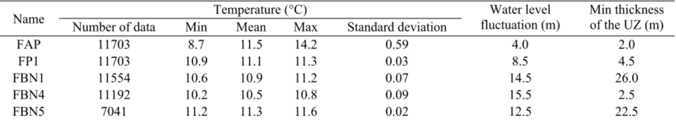
Seasonal water level fluctuations were highly variable on the study area (Table 2). The changes in water level between high and low water conditions in 2018 were down to < 5 m near river valley (FAP) but could reach up to 15 m on interfluve (FBN1, FBN4 and FBN5), with the thickness of UZ varying from 2 m (FAP) to 26 m (FBN1) (Table 2). The rise of water level was not simultaneous in different boreholes (Figure 2). In 2018, 4 boreholes (FBN4, FEP1, FP1 and FAP) reached their maximum levels in April, 4 boreholes (FA, FBN5, FVDV and FPM3) reached their maximum levels in March and 1
The Chalk aquifer exhibits a very inertial behavior, whereby the temporal variation curves of groundwater levels are smooth with rather gentle slopes except for FBN1, FBN5 and FAP (Figure 2). At FBN1 and FBN5, rapid drawdown was observed following pumping for water sampling during low water period (Figure 2). Large fluctuations in water levels were also observed during high water level period, probably related to nearby groundwater exploitation for industrial and agricultural purposes. In addition, at FBN5, rapid increases in water level were observed following rainfall events, particularly during high water level period in 2018. This could be explained by a direct infiltration of rainwater into the borehole due to bad conditions of the casing as reported by video observations during period of high soil moisture and intensive precipitation. At FAP, water level also rapidly increased following the rainfall events (Figure 2 and Figure 3) but with a low range (several decimeters). It increased about 1 hour after the rainfall and reaches a maximum value after 4 hours. Then it stabilizes gradually to its pre-disturbance level in the following tens of hours (Figure 3). The evolution of groundwater temperature and EC in this borehole follow the same pattern (Figure 3). The video observations show that the tube is in good condition, a direct intrusion of rainwater into this borehole is unlikely.
Table 2 : Summary of groundwater temperature and water table fluctuation from December 2017 to June 2019 (hourly data) measured by water-level loggers installed in unexploited boreholes and the minimum UZ thickness (derived from the water level in high water period in 2018).
Temperature (°C)
Name Number of data Min Mean Max Standard deviation fluctuation (m)Water level Min thickness of the UZ (m)
FAP 11703 8.7 11.5 14.2 0.59 4.0 2.0 FP1 11703 10.9 11.1 11.3 0.03 8.5 4.5 FBN1 11554 10.6 10.9 11.2 0.07 14.5 26.0 FBN4 11192 10.2 10.5 10.8 0.09 15.5 2.5 FBN5 7041 11.2 11.3 11.6 0.02 12.5 22.5 FEP1 11702 10.4 10.6 10.8 0.04 9.5 7.5 FPM3 11695 11.0 11.2 11.4 0.04 9.0 9.0 FVDV 11657 10.8 11.1 11.3 0.05 8.0 7.0 FA 11699 10.7 11.0 11.3 0.05 9.0 3.0
Figure 2: Rainfall (hourly data) and groundwater level from April 2017 to June 2019 (solid line: hourly data measured by water-level loggers; dashed line: water level curve drawn by monthly data)
Figure 3 : Response of groundwater level (hourly data), temperature (hourly data) and EC (hourly data) to a rainfall event (17mm at the 15th hour) at FAP from 5 July to 8 July 2018
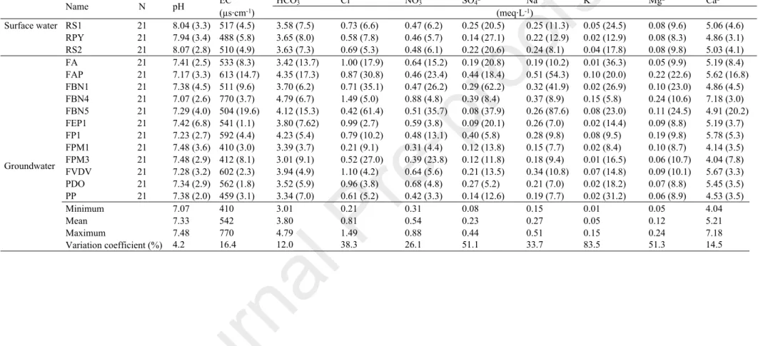
3.2 Chalk groundwater geochemistry
The chemical composition of the monitored groundwater is typical of the Chalk groundwater, with Ca2+ and HCO
3- being the dominant ions (Table 3). However, significant spatial and temporal
variations in groundwater geochemistry were observed, as shown by the variability of major ions concentrations and EC values. Average concentrations of Ca2+ and HCO
3- at each sampling site ranged
from 4.04 to 7.18 meq∙L-1 and from 3.01 to 4.79 meq∙L-1, respectively. For Cl- and NO
3- ions, the
average concentrations at each site ranged from 0.21 to 1.49 meq∙L-1 and from 0.31 to 0.88 meq∙L-1,
respectively. Concentrations of Mg2+, Na+, K+ and SO
42- were also variable but much lower than those
of other ions (Table 3). Temporal variations in concentrations were different for each major ion from one site to another.
Due to the high variability of the major ions concentrations, the mean values of EC at each site varied widely from 410 to 770 µs∙cm-1. Water samples collected at FBN4 were the most mineralized with the
FPM1 and FPM3 were the least mineralized with the lowest values of EC and low concentrations of major ions. The pH values of the groundwater samples were relatively homogeneous, with average values at each sampling site ranging from 7.07 to 7.48 (Table 3).
Surface water samples had the same Ca2+ - HCO
3- chemical facies as groundwater samples, as river
water in the study area comes mainly from drainage of the Chalk aquifer. The pH values (7.94 to 8.07) were higher than those measured in groundwater (7.07 to 7.48). The EC mean values at each site ranged from 488 to 517 µs∙cm-1, with relatively low spatial and temporal variabilities.
Table 3: Major ion concentrations and physicochemical parameters of Chalk groundwater from June 2017 to June 2019 (average values from monthly data) with the temporal variation coefficient (%) at each sampling point in blankets (N = Number of samples).
EC HCO3- Cl- NO3- SO42- Na+ K+ Mg2+ Ca2+ Name N pH (µs∙cm-1) (meq∙L-1) Surface water RS1 21 8.04 (3.3) 517 (4.5) 3.58 (7.5) 0.73 (6.6) 0.47 (6.2) 0.25 (20.5) 0.25 (11.3) 0.05 (24.5) 0.08 (9.6) 5.06 (4.6) RPY 21 7.94 (3.4) 488 (5.8) 3.65 (8.0) 0.58 (7.8) 0.46 (5.7) 0.14 (27.1) 0.22 (12.9) 0.02 (12.9) 0.08 (8.3) 4.86 (3.1) RS2 21 8.07 (2.8) 510 (4.9) 3.63 (7.3) 0.69 (5.3) 0.48 (6.1) 0.22 (20.6) 0.24 (8.1) 0.04 (17.8) 0.08 (9.8) 5.03 (4.1) FA 21 7.41 (2.5) 533 (8.3) 3.42 (13.7) 1.00 (17.9) 0.64 (15.2) 0.19 (20.8) 0.19 (10.2) 0.01 (36.3) 0.05 (9.9) 5.19 (8.4) FAP 21 7.17 (3.3) 613 (14.7) 4.35 (17.3) 0.87 (30.8) 0.46 (23.4) 0.44 (18.4) 0.51 (54.3) 0.10 (20.0) 0.22 (22.6) 5.62 (16.8) FBN1 21 7.38 (4.5) 511 (9.6) 3.70 (6.2) 0.71 (35.1) 0.47 (26.2) 0.29 (62.2) 0.32 (41.9) 0.02 (26.9) 0.10 (23.0) 4.86 (4.5) FBN4 21 7.07 (2.6) 770 (3.7) 4.79 (6.7) 1.49 (5.0) 0.88 (4.8) 0.39 (8.4) 0.37 (8.9) 0.15 (5.8) 0.24 (10.6) 7.18 (3.0) FBN5 21 7.29 (4.0) 504 (19.6) 4.12 (15.3) 0.42 (61.4) 0.51 (35.7) 0.08 (37.9) 0.26 (87.6) 0.08 (23.0) 0.11 (24.5) 4.91 (20.2) FEP1 21 7.42 (6.8) 541 (1.1) 3.80 (7.62) 0.99 (2.7) 0.59 (3.8) 0.09 (20.1) 0.26 (7.0) 0.02 (14.4) 0.09 (8.8) 5.19 (3.7) FP1 21 7.23 (2.7) 592 (4.4) 4.23 (5.4) 0.79 (10.2) 0.48 (13.1) 0.40 (5.8) 0.28 (9.8) 0.08 (9.5) 0.19 (9.8) 5.78 (5.3) FPM1 21 7.48 (3.6) 410 (3.0) 3.39 (3.7) 0.21 (9.1) 0.31 (4.4) 0.12 (13.8) 0.15 (7.7) 0.02 (8.4) 0.10 (8.7) 4.14 (3.5) FPM3 21 7.48 (2.9) 412 (8.1) 3.01 (9.1) 0.52 (27.0) 0.39 (23.8) 0.12 (11.8) 0.18 (9.4) 0.01 (16.5) 0.06 (10.7) 4.04 (7.8) FVDV 21 7.28 (3.2) 602 (2.3) 3.94 (4.9) 1.10 (4.2) 0.64 (5.6) 0.21 (13.5) 0.34 (10.8) 0.07 (14.8) 0.09 (10.1) 5.67 (3.3) PDO 21 7.34 (2.9) 562 (1.8) 3.52 (5.9) 0.96 (3.8) 0.68 (4.8) 0.27 (5.2) 0.21 (7.0) 0.02 (18.2) 0.07 (8.8) 5.45 (3.5) PP 21 7.38 (2.0) 459 (3.1) 3.34 (7.0) 0.61 (5.2) 0.42 (3.3) 0.14 (12.6) 0.19 (7.7) 0.02 (31.2) 0.06 (8.9) 4.53 (3.5) Minimum 7.07 410 3.01 0.21 0.31 0.08 0.15 0.01 0.05 4.04 Mean 7.33 542 3.80 0.81 0.54 0.23 0.27 0.05 0.12 5.21 Maximum 7.48 770 4.79 1.49 0.88 0.44 0.51 0.15 0.24 7.18 Groundwater Variation coefficient (%) 4.2 16.4 12.0 38.3 26.1 51.1 33.7 83.5 51.3 14.5
3.3 Groundwater dating by CFCs and SF6
3.3.1 Recharge temperature and excess air
In groundwater samples, Ne and Ar concentrations ranged from 0.84∙10-8 to 1.69∙10-8 mol∙L-1 and
1.71∙10-5 to 2.18∙10-5 mol∙L-1, respectively(Table 4). The recharge temperature and excess air were
estimated from the relationship between Ar and Ne (SI 2).
In May 2018, the estimated recharge temperature was similar in all waters of the study area with an average value of 10 °C. No recharge temperature information can be estimated at FBN4 due to a high value of excess air. In October 2018, the recharge temperature showed a spatial variability, with values ranging from 10 and 16 °C (with an average value of 13 °C), higher than that in May. This is consistent with several months’ winter recharge with relatively low temperatures, making the estimated recharge temperature in water samples in May lower than in October when samples were collected at the low water level with very few recharge in summer.
The estimated excess air in samples ranged from 0 to more than 8 ml∙L-1 with an average value of
about 3.4 ± 2 ml∙L-1. No significant difference in excess air values was observed between the two
sampling campaigns. At FPM1, negative excess air value was observed, which could probably due to the absorption by rubber tubes present at this borehole. The highest values of excess air were observed in water samples at FP1, FA, PP and FBN4, with the maximum value (> 8 ml∙L-1) for water sample
Table 4: CFCs, SF6, noble gases and estimated groundwater age by piston flow model, exponential mixing model (MRT = mean residence time) and binary mixing model (proportion of young and old water) in
May and October 2018 (the choices of the ideal model and estimated residence times are marked in bold; Cont.= contamination: \ = not applicable).
Piston flow model Exponential model (MRT years) Binary mixing model Name Sampling time SF6
(pptv) CFC-12 (pptv) CFC-11 (pptv) CFC-113 (pptv) Ar (10-5 mol∙L-1)
Ne
(10-8 mol∙L-1) SF
6 CFC-12 CFC-11 CFC-113 SF6 CFC-12 CFC-11 CFC-113 % young water young age old age Comment
May 9.7 522.7 205.5 56.6 1.93 1.32 6 24 34 31 0 7 25 27 75 0 40 FA Oct. 7.9 507.3 182.4 58.6 1.71 1.24 6 26 36 31 5 12 30 25 80 0 >50 May 7.1 538.0 278.0 62.4 1.83 1.16 8 11 25 30 8 \ \ 20 70 0 35 FAP Oct. 6.2 504.9 237.9 58.5 1.78 1.13 11 27 31 31 12 13.5 12 25 50 0 30
May 5.1 cont. cont. 66.4 1.72 1.03 16 \ \ 30 18 \ \ 18 40 0 30
FBN1
Oct. 5.3 cont. cont. 75.2 1.73 1.05 16 \ \ 28 18 \ \ 7 40 0 30
May 2.1 cont. 206.3 cont. 2.18 1.69 29 \ 34 \ 70 \ 25 \ 10 0 35
FBN4
Oct. 5.4 472.7 188.1 cont. 1.85 1.35 15 29 36 \ 17 17.5 30 \ 50 0 35
May 5.1 cont. cont. cont. 1.83 1.16 16 \ \ \ 18 \ \ \ \ \ \
FBN5
Oct. 4.0 cont. cont. 72.6 1.89 1.26 21 \ \ 29 30 \ \ 12 25 0 30 Not datable
May 5.4 cont. cont. 46.9 1.84 1.22 14 \ \ 33 16 \ \ 40 60 0 >30
FEP1
Oct. 5.1 cont. cont. 70.6 1.84 1.20 16 \ \ 29 19 \ \ 13.5 90 15 >60
May 7.5 cont. cont. 41.0 1.95 1.28 7 \ \ 33 6 \ \ 40 \ \ \
FP1
Oct. 3.6 376.1 cont. 46.2 1.77 1.21 23 34 \ 33 35 35 \ 40 30 0 40
May cont. cont. cont. 46.7 1.75 0.92 \ \ \ 33 \ \ \ 40 \ \ \
FPM1
Oct. cont. cont. cont. cont. 1.72 0.84 \ \ \ \ \ \ \ \ \ \ \ Not datable
May cont. cont. 141.8 cont. 1.77 1.08 \ \ 41 \ \ \ 50 \ \ \ \
FPM3
Oct. cont. cont. 95.9 cont. 1.74 1.04 \ \ 45 \ \ \ 100 \ \ \ \ Not datable
May 4.5 cont. 258.1 cont. 1.80 1.10 19 \ 15 \ 22 \ \ \ 30 0 30
FVDV
Oct. 3.9 cont. 239.4 cont. 1.70 1.04 22 \ 31 \ 35 \ 11 \ 25 0 30
May 5.1 504.5 163.9 49.9 1.72 0.99 16 26 38 32 18 12 40 35 30-50 0 >40 PDO Oct. 6.1 416.7 162.0 44.0 1.70 1.08 12 32 39 33 13.5 27 40 45 60 0 45 May 6.4 449.7 147.4 80.7 1.90 1.29 10 30 41 27 11 20 50 \ \ \ \ PP Oct. 6.9 376.1 135.4 cont. 1.88 1.41 9 34 42 \ 8.5 35 70 \ 65 0 >60
3.3.2 Groundwater apparent ages
The measured CFCs and SF6 concentrations in water samples (in pmol·L-1) were transferred to
atmospheric partial pressures (in pptv) according to Henry’s law. The data was rejected when calculated concentrations were greater than atmospheric peak concentrations (marked as contamination; Table 4).
A frequent contamination of tracer gases was observed on the study area, especially for CFC-12. Commonly recognized sources of CFCs contamination include seepage from septic tanks, landfills (Kjeldsen and Christophersen, 2001), release from polyurethane foam waste (Kjeldsen and Jensen, 2001), leaky sewer lines, leakage from underground storage tanks, infiltration or disposal of industrial wastes and recharge from rivers contaminated with CFCs (Cook et al., 2006). CFCs contamination could also result from agricultural activities. Agricultural application of pesticides may introduce CFCs, particularly CFC-11 to unsaturated air, as CFCs are allowed as inert ingredients in pesticide formulations (Plummer et al., 2000). In addition, CFCs can sorb into rubber and polymers; therefore water samples can also be contaminated with CFCs from contact with these materials such as permanently installed submersible pumps in wells with rubber parts (Cook et al., 2006; Dunkle et al., 1993). Although most SF6 concentrations did not exceed atmospheric peak concentrations, apparent
ages estimated by SF6 were generally much younger than all the other tracers, suggesting some
anthropogenic and/or natural addition of SF6. Anthropogenic sources of SF6 include high-voltage
electricity supply equipment, Mg and Al melting and landfills (Darling et al., 2012a; Santella et al., 2008). Unlike CFCs, which come exclusively from anthropogenic sources, SF6 can also be present
naturally in rocks. The major known source of terrigenous SF6 is found in fluorite and granite;
however, significant concentrations of SF6 is also reported in other mineral and rock types such as
contamination of CFCs and SF6. A small waste deposit site located near the borehole FBN1 (Figure 1)
could also represent a local source of pollution. Furthermore, since the majority of the study area is used as farmland, the agricultural application of pesticides could also be a potential source of contamination for CFCs, especially CFC-11 (Plummer et al., 2000). It should be noted that water samples collected at FPM1 were contaminated by all the 4 trace gases. Indeed, FPM1 is a private well in a farm where a permanently pumping system is installed. Water samples were collected directly from the tap. Air contact with the pumped water may occur between the pump and the tap. Rubber water tubes connected with the tap could also present a potential source of contamination. As a result of frequent contamination, some water samples are not datable (FBN5, FPM1 and FPM3) as only one or two tracers are valid for calculation and estimated ages are not consistent for different tracer gases.
Cross-plots of concentrations for CFC-11 vs CFC-113 and SF6 vs CFC-113 super imposed on the
mixing models have been realized (SI 3). CFC-12 is not used for cross-plot due to its frequent contamination. Also, not all water samples were plotted as some of them were concerned by contamination of related tracers with concentrations surpassing the range of axis. The plot position of sampling points compared to PFM, EMM and BMM curves allowed to provide information for the selection of models. Also, the consistency of apparent ages between different tracer gases and between the two sampling campaigns is used for the validation of models. When different tracers did not give consistent apparent ages, values estimated by CFC-11 and CFC-113 were considered to be more reliable than CFC-12 and SF6 as the latter two tracers were largely influenced by anthropogenic
activities on the study area.
The selected mixing models and estimated residence time are resumed in Table 4. Groundwater residence time of the study area is rather heterogeneous, ranging from modern to about 50 years. This result is comparable with previously published data on the Champagne Mount area, with an average residence time of about 25 years (Mangeret et al., 2012). The piston flow model is more suitable for FEP1 and PP (30 to 40 years). The exponential mixing model is the best model for FBN1, FBN4 and FP1 (MRT from 18 to 40 years). The binary mixing model is more suitable for FA, FAP, FVDV and PDO (25% to 80% of modern water and an end member of old water ranging from 30 to more than 50
years). Residence times estimated by piston flow and exponential mixing model at each point were similar between the sampling campaign of May 2018 (high water) and October 2018 (low water). For boreholes applying the binary mixing model, significant differences of residence time were observed between the two sampling campaigns. At FA, FAP and FVDV, estimated apparent ages for samples collected in May are younger than in October with higher proportions of modern water or younger ages of the old end member. At PDO, apparent ages for samples collected in May are older than in October with less proportions of modern water (age < 10 years) (Table 4).
4 Discussion
4.1 Hydrodynamic characteristics
The unconfined Chalk aquifer of the study area possesses highly heterogeneous hydrological characteristics. A higher variation in water levels was observed on interfluves than in river valleys (Figure 2) attesting differences in transmissivity and storage yield. In river valleys, high density of active fractures are consistently developed, resulting in high permeability of the aquifer (Haria et al., 2003; Ineson, 1962; Price, 1987; Price et al., 1993). Water is discharged quickly through the fractures toward the valleys at times of high recharge, thus not allowing the water levels to rise significantly (Allen et al., 1997; Whitehead and Lawrence, 2006). Conversely, on interfluves, the low permeability and storage yield make the Chalk aquifer more sensitive to recharge and discharge, resulting in greater and faster water level fluctuations between low water and high water periods (Allen et al., 1997). In general, groundwater reached the maximum level earlier on interfluves than in river valleys, which is reasonable as on interfluves the distance to the groundwater divide line is closer and the time of lateral flow from the recharge zones towards the borehole is shorter.
observed, suggesting a dominant recharge through the Chalk matrix, as demonstrated by numerous studies in Chalk aquifers (e.g., Barhoum, 2014; Haria et al., 2003; Ireson et al., 2006; Mathias et al., 2006; Smith et al., 1970; Wellings and Bell, 1980). However, differences are observed at FAP. Sharp increases in water level after rainfall events were observed, followed by equally rapid declines. Figure 3 shows an example of this trend in July 2018. Water level started to increase about 1h after the rainfall event and reached its maximum value about 4h later (85.45 to 85.67 m NGF). Similar rapid responses within 24h of rainfall were observed in a few previous investigations (Allen et al., 1997; Lee et al., 2006). Allen et al. (1997) suggested that this would be expected only if the large fractures had been replenished (rapid transfer initiated) and subsequently drained during recharge period. At FAP, hourly temperature and EC were also measured and compared with rainfall time series. Water temperature increased about 2h after the rainfall and reached its maximum value about 7h later (11.6 to 12.2°C). EC decreased about 2h after precipitation and reached the minimum value about 9h later (625 to 460 µS.cm-1). In July (summer), the increase in temperature may be easily explained by a
higher atmospheric temperature in July compared with groundwater temperature. EC decreased due to the dilution by rainwater. The variation of temperature and EC combining with that of water level confirms that the aquifer at FAP testifies to rapid transfers via a well-developed fracturing network thus exhibits no longer an inertial behavior. Note that the response of water level was faster than that of temperature and EC, as the water pressure transfer process was faster than the mixing between rainwater and groundwater. Rapid flows through fractures are added to matrix flows that are still effective as evidenced by the evolution of groundwater levels on an annual scale (Figure 2).
Excess air in groundwater provides also useful information on flow pathways and recharge processes. Higher excess air values were measured in groundwater at FP1, FA, PP and FBN4. These 4 boreholes have a thin UZ (less than 5 m in 2018 high water period; Table 2). The water level at pumping station PP is not measured, but historical data showed a UZ thickness of about 5 m (data source: InfoTerre.brgm.fr). It is suggested that at these 4 shallow groundwater sites, recharge by preferential fracture flow is favored with more fractures developed near the surface, while the other deeper groundwater sites are dominated by matrix flow as fracturing of the chalk decreases with depth (Haria
et al., 2003; Mathias et al., 2006). The preferential flow is guaranteed by water-filled small fractures and the capillary channels above the water table, resulting in a subsequent rapid rise of water table after rainfalls (Heaton and Vogel, 1981). These effects are supposed to favor the formation and entrapment of air bubbles, which could possibly explain the higher quantity of excess air in water samples collected at these points. Note that the borehole FAP also has a water table depth of less than 5 m. However, the excess air values in water were relatively low, similar to the mean value of the study (SI 2). This is consistent with the very developed fracturing network at FAP. Large fractures are less favorable for the air entrapment, resulting in relatively low excess air values than other shallow groundwater sites.
4.2 Origin of major ions
The correlation matrix of major ions (details of the calculation method and results can be found in SI 4 and 5) and relationships between ions (Figure 4) were used to study the origin of major ions. Concentrations of Ca2+ and HCO
3- ions are significantly correlated (Figure 4a and SI 5), which is
consistent with the typical chemistry of Chalk groundwater. However, Ca2+ / HCO
3- plots (Figure 4a)
are not aligned to the 1:1 line (Edmunds et al., 1987) with an enrichment of Ca2+ compared with HCO 3-,
indicating a secondary origin of Ca2+ in addition to Chalk dissolution (Barhoum et al., 2014). Ca2+
excess compared with HCO3- was then plotted with the sum of Cl-, NO3- and SO42- (Figure 4b). Most
data points are plotted along the 1:1 line, implying that Ca2+ excess may be due to an agricultural
source as Cl-, NO
3- and SO42-. Indeed, a common agriculture source of Cl-, NO3- and SO42- is also
indicated by a significant correlation between these ions (SI 5). In fact, lime (CaO) can be used in agricultural to optimize field pH (Aquilina et al., 2012; Bolan et al., 2003) and some fertilizers could contain CaO or Ca2+ as secondary or minor component (such as TSP-SUPER 45 used in the
impurities and clay minerals in superficial formations (mainly colluvium and alluvium in the study area) may provide Mg2+, K+ as well as SO
42- to groundwater (Gillon et al., 2010; Stuart and Smedley,
2009).
Figure 4 : (a) Ca2+ versus HCO
3- (solid line 1:1 represents the Chalk dissolution line); (b) [Ca2+ - HCO3-] versus [NO3- + Cl- +
SO42-]; (c) Cl- versus Na+ (solid line 1:1 represents the meteoric water line)
4.3 Spatial and temporal variations of Chalk groundwater geochemistry under effects of hydrogeological setting and residence time
4.3.1 Spatial analyses
To interpret the spatial distribution of Chalk groundwater geochemistry, a principal component analysis (PCA) of major ion concentrations and EC was performed (details of the method can be found in SI 4) (Figure 5). The first two principal components (F1 and F2) justified together 78% of the variance. F1 is positively weighted on the allochthonous agricultural ions (NO3- and Cl-) and on Ca2+
(more weakly) and negatively weighted on Na+, Mg2+, SO
42-, K+ and HCO3-, which are interpreted as
autochthonous ions. F2 is positively weighted on EC and all the major ions but the most strongly on Ca2+ and HCO
3-, which correspond to the typical geochemistry of Chalk groundwater dominated by
these two ions.
Hierarchical clustering of PCA shows a vast spatial heterogeneity of major ion concentrations on the study area and distinguishes six water-type groups (Figure 5). RS1, RS2 and RPY (river waters) were plotted near the center zone of PCA graph, implying that the geochemistry of river water was similar to the average condition of groundwater, which is justified by the drainage of the whole aquifer by the rivers. Relatively low concentrations of agricultural ions (NO3-, Cl- and Ca2+) were observed at FBN1
and FBN5, which could be explained by the large UZ thickness (> 20 m; Table 2), whereby the aquifer tended to be less influenced by agriculture activities (e.g., fertilizer applications). In contrast, higher concentrations of agricultural ions were observed at FVDV, PDO, FA and FEP1 because of smaller UZ thickness (< 10m; Table 2). Extremely high major ion concentrations at FBN4 were supposed to be related to the landfill located upstream, representing an important point source of pollution. FP1 and FAP have a similar chemical composition with high concentrations on Na+, Mg2+, SO
42- and K+
ions especially. At these two points, the Chalk is covered by a large surface of colluvium with relatively high content on clay minerals (Figure 1), which represents a possibly source of these ions in groundwater. Low concentrations of major ions were observed at FPM1, FPM3 and PP, which could be explained by the presence of superficial formations (graveluche and alluvium) limiting the transfer of water and solute from surface to the aquifer (Linoir, 2014). The impact of superficial formations overlying the Chalk on groundwater geochemistry are further discussed in the following section.
4.3.2 Temporal variations
The temporal variation of geochemistry was explored by analyzing the EC chronicle compared with groundwater level time series (Figure 6). A combination of hydrogeological setting, residence time and land use information was used to explain the temporal variations of Chalk geochemistry on the study area.
Area with large fluctuation in water level
Large fluctuation in water level was observed at FBN1 and FBN5 (> 12 m; Table 2). EC time series were highly correlated with water level fluctuations (Figure 6 and Table 5). During high water level period in 2018, water level increased substantially following intensive recharge, resulting in an increase in EC of about 150 and 300 µs∙cm-1 at FBN1and FBN5 respectively. However, no significant
variation of EC was observed during high water level period in 2019, as water level was much lower under dry climate conditions. According to groundwater dating, the groundwater flow was described by the exponential mixing model and a MRT of 18 years was estimated at FBN1 (no accurate age was deduced for FBN5), indicating a spatially uniform recharge and a mixture of different flows. In this context, contaminants concentrated near the land surface area infiltrated progressively across the UZ following recharge. Under low water level conditions, the contamination front was disconnected with the SZ. It transferred slowly downward through the unsaturated Chalk matrix. Meanwhile, solutes in the SZ were diluted by the mixing process of groundwater, so that a low EC was observed. As water level rose and reached the contamination front, the contamination source was re-activated and contaminants concentrations increased rapidly in the SZ so that a high EC was observed. Similar pollutant remobilization processes were previously suggested by Brouyère et al. (2004), Hakoun et al. (2017) and Orban et al. (2010). The highly correlation between time series of NO3-, Cl-, SO42-, Ca2+
concentrations and water level fluctuation (Table 5) confirms this mechanism.
At FBN4, a high correlation between EC and large water level fluctuation (15.5m; Table 2) was also observed in a context of exponential mixing (MRT = 17 years; Table 4). However, the temporal variation of EC followed that of water level during the whole monitoring period (2017-2019) while EC remained stable at low water levels at FBN1 and FBN5. This could be explained by the thin UZ at
FBN4 (2.5m; Table 2), whereby the contaminated area was always partially submerged by groundwater level even during low water level period.
At FVDV, the water level fluctuation was smaller (8 m; Table 2), resulting in a lower correlation between EC and water level times series (r = 0.69; Table 5) compared to FBN1, FBN4 and FBN5. Groundwater consisted mainly of 30-year-old water mixed with 25-30% of modern water, suggesting small contributions of rapid recharge through fractures.
Area with developed fracture network and low UZ thickness
EC time series were inversely related to water level fluctuation at FAP and FA (Figure 3 and Figure 6), suggesting that the dilution effect was the most important factor that influences the geochemistry. At these two sites, the UZ thickness was low (< 3 m; Table 2) and fractures were supposed to be developed near surface area. Groundwater dating showed 50-70% and 75-80% of modern water at FAP and FA respectively by the binary mixing model (Table 4), indicating an aquifer constituted mainly by freshly percolated rainwater that favors the process of dilution. Larger proportion of modern water at FA could be explained by its location close to groundwater divide line, receiving few lateral flow. It should be noted that, even during high water level period, the groundwater at FAP and FA was composed of 20% to 50% of old water aged over 30 years. This older end-member is linked to the lateral flow originated from upstream recharge areas.
Area with superficial formation
EC values were stable in time at FPM1 and FEP1 (Figure 6). Groundwater dating showed a residence time of > 30 years at FEP1 in a piston flow context, indicating a small recharge area away from the site (no accurate age was deduced for FPM1; Table 4). These two wells are situated in the north of the study area, where large surfaces of the Chalk are covered by graveluche (Figure 1). The graveluche
laterally in the SZ during more than 30 years, resulting in a stable geochemistry independent on water level fluctuation. At FPM3 (downstream the borehole FPM1; Figure 1), a time lag was observed between EC and water level time series, as a result of delayed solute transfer by the discontinuous graveluche formations. At PP, EC was also stable with a residence time of about 40 years estimated by a piston flow model (Table 4). With a high proportion of clayey minerals, the alluvium can play the same role as graveluche as a flow barrier on the Chalk. Moreover, the deep screen position of PP (23-80 m; Table 1) allowed pumping of deep groundwater with longer residence time. Previous studies (e.g., Barhoum et al. 2014; El Janyani et al. 2012) have shown that other superficial formations such as flint clay layers can have similar impacts on Chalk aquifers.
Area along riverside
PDO is a pumping station used for drinking water supply located close to the Suippe River (Figure 1). The drawdown of groundwater level due to intensive exploitation could result in a recharge of aquifer by river water, as testified by a higher proportion of modern water in October than in May 2018 (Table 4). Indeed, the groundwater level was lower in October resulting in increased flow from the river to the aquifer. The EC of river water was relatively stable, making the EC at PDO stable over time (Figure 6).
FP1 is a non-exploited borehole located in the Vesle River valley (Figure 1). No correlation relationship between EC and water level was observed. Located far from the groundwater divide line, FP1 has a very large recharge area, receiving groundwater of different residence times (a mean residence time of 35-40 years was estimated in an exponential mixing context; Table 4). As a result, groundwater chemistry was greatly buffered and EC was poorly related to water level fluctuation (Figure 6).
Figure 6 : Temporal variation of groundwater level and EC (monthly data from June 2017 to June 2019)
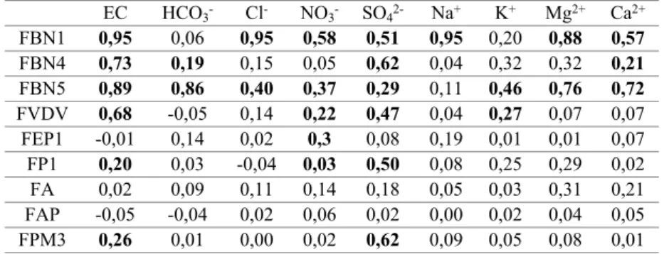
Table 5: Correlation coefficient (r2) of EC and all major ions with groundwater level (statistically significant as the P-value <
0.05, related r2 values when P-value < 0.05 are marked in bold; calculation details are presented in SI 4 and 6).
EC HCO3- Cl- NO3- SO42- Na+ K+ Mg2+ Ca2+
FBN1 0,95 0,06 0,95 0,58 0,51 0,95 0,20 0,88 0,57 FBN4 0,73 0,19 0,15 0,05 0,62 0,04 0,32 0,32 0,21
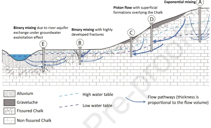
4.4 A conceptual model of aquifer functioning
A conceptual model of unconfined Chalk aquifer (Figure 7) was established in order to explore how hydrogeological settings including fracture distribution, groundwater level depth, superficial formations and aquifer-river relationship can influence the hydrogeological functioning of the aquifer in terms of flow pathways, mixing process, residence time and groundwater geochemistry variation.
In general, under deep groundwater level conditions, the geochemistry of the aquifer tends to be less influenced by near surface contaminations with relatively low concentrations of agriculture ions. This situation usually occurs on interfluves, near the groundwater divide line (Figure 7A). If no superficial formations overlay on the Chalk, the aquifer receives a spatially uniform recharge and an exponential mixing model could be applied with a relatively short residence time. As transmissivity and storage yield are low on interfluve with a thick UZ, groundwater level fluctuations are important, leading to levels of contamination positively correlated to water table dynamics.
At shallow groundwater sites, the thin UZ of Chalk aquifer is usually highly fractured (Figure 7B). Rapid recharge through fractures is favored, making groundwater a mixture of freshly percolated water and old water coming from upstream recharge area, as demonstrated by a binary mixing model. The shallow groundwater sites with high proportion of modern water mainly locate in river valleys (where fracture networks are well developed) but could also present on interfluves. At these sites, groundwater geochemistry is mostly influenced by the dilution effects of rainfall, leading to mineralization degree of groundwater negatively correlated to water table dynamics.
Superficial formations overlaying on the Chalk such as graveluche, colluvium and alluvium have important effects on groundwater flow and geochemistry. These superficial formations are usually intermitted and constituted by high content of clayey minerals, presenting a lower permeability than the Chalk. They could consequently constitute a barrier limiting the rapid recharge of water and solute into the aquifer. At these sites, a piston flow model better describes the groundwater flow and relatively old groundwater ages are estimated, which could explain the stable or delayed groundwater geochemistry with respect to water table fluctuations (Figure 7C and D).
For sites near rivers where groundwater is exploited, the exchange between groundwater and river water should be considered (Figure 7E). The recharge of aquifer by rivers could occur, especially during low water level period, leading to groundwater geochemistry influenced by surface water.
Figure 7 : Schematized hydrogeological functioning of unconfined Chalk aquifers
5 Conclusion
The present study brings out interesting implications for the hydrogeological functioning of unconfined Chalk aquifers, by an approach combining hydrodynamic, geochemical and groundwater dating tools. Based on an intensive sampling network on a watershed scale, groundwater level fluctuations and chemical compositions (major ions concentrations) were monitored continuously during two years (2017-2019).
Groundwater dating using CFCs and SF6 was also realized for the first time in this unconfined Chalk
aquifer. Despite the frequent contaminations of CFCs and SF6 detected on the study area, relevant
information on residence times and mixing processes of the Chalk groundwater was obtained at the majority of sites. The aquifer is made up of waters of different ages ranging from less than 20 years to more than 50 years, with piston flow, exponential or binary mixing models defined at each sampling site implying for different flow pathways and mixing processes in the aquifer.
Despite the Ca2+ - HCO
3- chemical facies, a high spatial and temporal heterogeneity of groundwater
geochemistry in the unconfined Chalk aquifer was highlighted on the study area. Different correlation relationships between the EC time series and groundwater level fluctuations were observed: correlated, anti-correlated or independent. These variabilities were explained by a combined effect of water level fluctuation, groundwater residence time, thickness of the UZ, superficial formations, distribution of fracturing network, aquifer-river relationships and human activities.
The combination of different tools allowed the establishment of a conceptual model of chalk aquifer functioning. The multi-tool methodology developed in this study and the established conceptual model might be used in Chalk aquifers or other multi-porosity mediums for the prediction of spatial and temporal variations of groundwater mineralization and solutes transport (natural or anthropogenic) and for the evaluation of aquifer vulnerability. However, the used methods still have some limitations. Firstly, the two-year long time series of groundwater level and geochemical parameters are relatively short to interpret a general and comprehensive mechanism of aquifer functioning. Then, the age-dating was disturbed by the contamination of tracers, resulting in the missing of groundwater flow information at some sites. Also, the methods focus mostly on a qualitative rather than a quantitative perspective, which could limit its application on contaminant transport prediction. Therefore, further investigations would be necessary. The monitoring of groundwater level fluctuations and geochemistry can be continued to obtain longer times series, with the aim to study the influence of different climate conditions on the Chalk aquifer functioning in a climate change context. With respect to groundwater dating, tritium analysis could be a good complement for CFCs and SF6, especially for
sites contaminated by several tracers. At last, the hydrodynamic and geochemical numerical modeling tool, based on the conceptual model established in the study, could be a relevant complement.
Declaration of Competing Interest
The authors declare that they have no known competing financial interests or personal relationships that could have appeared to influence the work reported in this paper.
Acknowledgements
This work was co-funded by the BRGM, the Agence de l'Eau Seine-Normandie, the Region Grand-Est, the Grand-Reims Metropole and ARS Grand-Est. Authors would also like to thank the owners and operators for access to their boreholes.
Supplementary data
Supplementary data to this article can be found online.
References
ADES Database, 2019. ADES: le portail national d’Accès aux Données sur les Eaux Souterraines pour la France métropolitaine et les départements d’outre-mer. https://ades.eaufrance.fr/. Accessed date: 22 July 2019.
Aeschbach‐Hertig, W., Peeters, F., Beyerle, U., Kipfer, R., 1999. Interpretation of dissolved atmospheric noble gases in natural waters. Water Resources Research 35, 2779–2792. https://doi.org/10.1029/1999WR900130
Allen, D.J., Brewerton, L.J., Coleby, L.M., Gibbs, B.R., Lewis, M.A., MacDonald, A.M., Wagstaff, S.J., Williams, A.T., 1997. The physical properties of major aquifers in England and Wales (Technical Report No. WD/97/34). British Geological Survey.
Allshorn, S.J.L., Bottrell, S.H., West, L.J., Odling, N.E., 2007. Rapid karstic bypass flow in the unsaturated zone of the Yorkshire chalk aquifer and implications for contaminant transport.
Geological Society, London, Special Publications 279, 111–122.
Aquilina, L., Ayraud, V., Labasque, T., Le Corre, P., 2006. Dosage des composés chlorofluorocarbonés et du tétrachlorure de carbone dans les eaux souterraines. Application à la datation des eaux, 51 p.
Aquilina, L., Ladouche, B., Doerfliger, N., Bakalowicz, M., 2003. Deep Water Circulation, Residence Time, and Chemistry in a Karst Complex. Groundwater 41, 790–805. https://doi.org/10.1111/j.1745-6584.2003.tb02420.x
Aquilina, L., Poszwa, A., Walter, C., Vergnaud, V., Pierson-Wickmann, A.-C., Ruiz, L., 2012. Long-Term Effects of High Nitrogen Loads on Cation and Carbon Riverine Export in Agricultural Catchments. Environ. Sci. Technol. 46, 9447–9455. https://doi.org/10.1021/es301715t
Ayraud, V., Aquilina, L., Labasque, T., Pauwels, H., Molenat, J., Pierson-Wickmann, A.-C., Durand, V., Bour, O., Tarits, C., Le Corre, P., Fourre, E., Merot, P., Davy, P., 2008. Compartmentalization of physical and chemical properties in hard-rock aquifers deduced from chemical and groundwater age analyses. Applied Geochemistry 23, 2686–2707. https://doi.org/10.1016/j.apgeochem.2008.06.001
Bakalowicz, M., 2018. De l’évolution historique du concept d’aquifère de la craie. Géologues 199, 4– 6.
Baran, N., Chabart, M., Braibant, G., Joublin, F., Pannet, P., Perceval, W., Schimidt, C., 2006. Détermination de la vitèsse de transfert des nitrates en zone crayeuse sur 2 bassin versants à enjeux : La retourne (08) et la Superbe (51). Rapport BRGM/RP-54985-FR, 109 p.
Baran, N., Lepiller, M., Mouvet, C., 2008. Agricultural diffuse pollution in a chalk aquifer (Trois Fontaines, France): Influence of pesticide properties and hydrodynamic constraints. Journal of Hydrology 358, 56–69. https://doi.org/10.1016/j.jhydrol.2008.05.031
Barhoum, S., 2014. Transferts dans la craie : approche régionale : le Nord-Ouest du Bassin de Paris : approche locale : la carrière de Saint-Martin-le-Noeud (phdthesis). Université Pierre et Marie Curie - Paris VI, 334 p.
Barhoum, S., Valdès, D., Guérin, R., Marlin, C., Vitale, Q., Benmamar, J., Gombert, P., 2014. Spatial heterogeneity of high-resolution Chalk groundwater geochemistry – Underground quarry at Saint Martin-le-Noeud, France. Journal of Hydrology 519, 756–768. https://doi.org/10.1016/j.jhydrol.2014.08.001
Barraclough, D., Gardner, C.M.K., Wellings, S.R., Cooper, J.D., 1994. A tracer investigation into the importance of fissure flow in the unsaturated zone of the British Upper Chalk. Journal of Hydrology 156, 459–469. https://doi.org/10.1016/0022-1694(94)90090-6
Bolan, N.S., Adriano, D.C., Curtin, D., 2003. Soil acidification and liming interactions with nutrientand heavy metal transformationand bioavailability, in: Advances in Agronomy, Advances in Agronomy. Academic Press, pp. 215–272. https://doi.org/10.1016/S0065-2113(02)78006-1
Brouyère, S., 2006. Modelling the migration of contaminants through variably saturated dual-porosity, dual-permeability chalk. Journal of Contaminant Hydrology 82, 195–219. https://doi.org/10.1016/j.jconhyd.2005.10.004
Brouyère, S., Dassargues, A., Hallet, V., 2004. Migration of contaminants through the unsaturated zone overlying the Hesbaye chalky aquifer in Belgium: a field investigation. Journal of Contaminant Hydrology 72, 135–164. https://doi.org/10.1016/j.jconhyd.2003.10.009
Busenberg, E., Plummer, L.N., 2000. Dating young groundwater with sulfur hexafluoride: Natural and anthropogenic sources of sulfur hexafluoride. Water Resources Research 36, 3011–3030. https://doi.org/10.1029/2000WR900151
Busenberg, E., Plummer, L.N., 1992. Use of chlorofluorocarbons (CCl3F and CCl2F2) as hydrologic tracers and age-dating tools: The alluvium and terrace system of central Oklahoma. Water Resources Research 28, 2257–2283. https://doi.org/10.1029/92WR01263