Global trends in visibility: implications for dust sources

(1)

HAL Id: hal-00302624

https://hal.archives-ouvertes.fr/hal-00302624

Submitted on 27 Feb 2007

HAL is a multi-disciplinary open access

archive for the deposit and dissemination of sci-entific research documents, whether they are pub-lished or not. The documents may come from teaching and research institutions in France or abroad, or from public or private research centers.

L’archive ouverte pluridisciplinaire HAL, est destinée au dépôt et à la diffusion de documents scientifiques de niveau recherche, publiés ou non, émanant des établissements d’enseignement et de recherche français ou étrangers, des laboratoires publics ou privés.

Global trends in visibility: implications for dust sources

N. M. Mahowald, J. A. Ballantine, J. Feddema, N. Ramankutty

To cite this version:

N. M. Mahowald, J. A. Ballantine, J. Feddema, N. Ramankutty. Global trends in visibility: implica-tions for dust sources. Atmospheric Chemistry and Physics Discussions, European Geosciences Union, 2007, 7 (1), pp.3013-3071. �hal-00302624�

(2)

ACPD

7, 3013–3071, 2007

Global trends in visibility: implications for dust

sources N. M. Mahowald et al. Title Page Abstract Introduction Conclusions References Tables Figures ◭ ◮ ◭ ◮ Back Close Full Screen / Esc

Printer-friendly Version Interactive Discussion Atmos. Chem. Phys. Discuss., 7, 3013–3071, 2007

www.atmos-chem-phys-discuss.net/7/3013/2007/ © Author(s) 2007. This work is licensed

under a Creative Commons License.

Atmospheric Chemistry and Physics Discussions

Global trends in visibility: implications for

dust sources

N. M. Mahowald1, J. A. Ballantine2,*, J. Feddema3, and N. Ramankutty4

1

National Center for Atmospheric Research, Boulder Colorado, USA

2

Institute for Computational Earth System Science, University of California, Santa Barbara, CA, USA

3

Department of Geography, University Kansas, Lawrence, Kansas, USA

4

Department of Geography, McGill University, Montreal, Quebec, Canada

*

now at: United States Geological Survey, Denver, Colorado, USA

Received: 8 January 2007 – Accepted: 21 February 2007 – Published: 27 February 2007 Correspondence to: N. M. Mahowald ([email protected])

(3)

ACPD

7, 3013–3071, 2007

Printer-friendly Version Interactive Discussion

Abstract

There is a large uncertainty in the relative roles of human land use, climate change and carbon dioxide fertilization in changing desert dust source strength over the past 100 years, and the overall sign of human impacts on dust is not known. We used visibility data from meteorological stations in dusty regions to assess the anthropogenic impact 5

on long term trends in desert dust emissions. Visibility data are available at thou-sands of stations globally from 1900 to the present, but we focused on 359 stations with more than 30 years of data in regions where mineral aerosols play a dominant role in visibility observations. We evaluated the 1974 to 2003 time period because most of these stations have reliable records only during this time. We first evaluated 10

the visibility data against AERONET aerosol optical depth data, and found that only in dusty regions are the two moderately correlated. Correlation coefficients between visibility derived variables and AERONET optical depths indicate a moderate correla-tion (∼0.47), consistent with capturing about 20% of the variability in optical depths. Two visibility derived variables appear to compare the best with AERONET observa-15

tions: the fraction of observations with visibility less than 5 km (VIS5) and the surface extinction (EXT). Regional trends show that in many dusty places, VIS5 and EXT are statistically significantly correlated with the palmer drought severity index (based on precipitation and temperature) or surface wind speeds, consistent with dust temporal variability being largely driven by meteorology. This is especially true for North African 20

and Chinese dust sources, but less true in the Middle East, Australia or South America, where there are not consistent patterns in the correlations. Climate indices such as El Nino or the North Atlantic Oscillation are not correlated with visibility derived variables in this analysis. There are few stations where visibility measures are correlated with cultivation or grazing estimates on a temporal basis, although this may be a function of 25

the very coarse temporal resolution of the land use datasets. On the other hand, spatial analysis of the visibility data suggests that natural topographic lows are not correlated with visibility, but land use is correlated at a moderate level. This analysis is consistent

(4)

ACPD

7, 3013–3071, 2007

Printer-friendly Version Interactive Discussion with land use being important in some regions, but meteorology driving interannual

variability during 1974–2003.

1 Introduction

Mineral aerosols or desert dust particles are hypothesized to be important for local health and air quality problems, as well as impacts on the global environment through 5

changes in the radiative budget, precipitation processes, atmospheric chemistry and biogeochemistry (e.g. Rosenfeld and Nirel, 1996, Dentener, et al., 1996, Miller and Tegen, 1998, DeMott, et al., 2003, Jickells, et al., 2005). While mineral aerosol sources are thought to be dominated by natural processes (e.g. Prospero et al., 2002), the pos-sibility of human impacts on mineral aerosols cannot be eliminated by the existing data 10

(Mahowald and Dufresne, 2004; Tegen et al., 2004; Mahowald et al., 2004; Mahowald, et al., 2005). On small scales, cultivation or pasture usage has been shown to increase the availability of particles for wind erosion (e.g. Gillette, 1988, Neff, et al., 2005). In addition, ice core records show that dust is sensitive to climate change (e.g. Petit and al., 1999). Thus, human influenced climate change and land use may be impacting 15

dust concentrations. Finally, plants are thought to be better able to deal with water stress under a higher carbon dioxide environment, suggesting that desert extent (and presumably therefore dust) may be decreasing over the last century as carbon diox-ide levels increase (e.g. Smith, et al., 2000; Mahowald and Luo, 2003). Attempts to determine the impacts of global scale anthropogenic land use on dust emissions are 20

hampered by the similarity in the spatial distribution of land use derived dust and natu-ral dust for some sources (e.g. Mahowald et al., 2002; Luo et al., 2003; Mahowald, et al., 2004). Results of modeling simulations suggest that humans have either increased or decreased dust since preindustrial times, depending on the relative importance of human land use, carbon dioxide fertilization and climate change in driving dust (Ma-25

howald and Luo, 2003). Ice core changes between the preindustrial and current time periods are not consistent within regions and cannot differentiate between these

(5)

ACPD

7, 3013–3071, 2007

Printer-friendly Version Interactive Discussion ent processes (Mahowald and Luo, 2003).

One long time series dataset that is globally available is visibility data collected at meteorological stations. It has been used in many previous studies (e.g. Middleton, 1984; McTainsh et al., 1989; Goudie and Middleton, 1992; Sun et al., 2001; Engel-staedter et al., 2003). However, visibility data have not been compiled and presented 5

globally with time trends in previous studies. These data are available at hourly to sev-eral times daily intervals over much of the last century at many meteorological stations located throughout the world. One problem with these data is that visibility is not di-rectly related to aerosol concentration, but may be influenced by humidity, cloudiness or rain. In addition, aerosol amount near a station may be impacted by very local effects, 10

such as the existence of a dirt road nearby, as well as the potential for other problems (e.g. Middleton et al., 1985). Thus as a first step in our analysis, we compared the visibility data against other aerosol data (AERONET aerosol optical depths: Holbren et al., 2001) to understand the quantitative value of this dataset.

Many processes may be important for the generation of atmospheric dust, includ-15

ing strong winds, precipitation, drought conditions, land surface properties, and human land use. For each of these processes we try to derive a representative proxy from a global dataset. However, this approach has fundamental limitations due to lack of qual-ity data. There is a large spatial variabilqual-ity in surface winds and precipitation, making these variables difficult to constrain globally (e.g. Dai et al., 1996). Very little is know 20

globally about land surface properties, and we address these in a future study. Espe-cially problematic are datasets on the time evolution of human cultivation and grazing. The datasets used here present a broad view of the time evolution of cultivation and grazing, and represent the best datasets available (Klein-Goldewijk, 2001; Ramankutty and Foley, 1999). However they are interpolations between land use censuses taken 25

every 5 years in the best case, and often every 10 years or longer, and therefore crudely represent the time record of human land use. In addition, it is not clear how human land use would impact dust. Some studies have shown that cultivation and grazing make soils much easier to deflate (Gillette, 1988; Neff et al., 2005). Soil conservation

(6)

ACPD

7, 3013–3071, 2007

Printer-friendly Version Interactive Discussion efforts such as trees planted to block the winds, contour plowing, and leaving dead

vegetation on the top of the soils have been shown to be effective in reducing wind erosion (citation). Thus, it is not always straightforward to deduce what the relationship should be between human land use and dust.

Our goal in this paper is to use visibility data for estimating long term trends in 5

aerosols, especially desert dust aerosols. We describe our methods in Sect. 2. We first evaluate several proxies derived from the hourly visibility data against AERONET column aerosol optical depth data in Sect. 3. Then we use visibility proxies to look at temporal trends in dusty regions. Finally, we correlate visibility proxies with meteoro-logical variables such as precipitation and wind speeds as well as the human driven 10

variables, estimated cultivation and grazing use (Sect. 4). Summary and conclusions are presented in Sect. 5.

2 Methodology

For this paper, we analyze hourly to several times daily station data from the DSS 463.3 surface weather observation dataset created by the National Climatic Data Cen-15

ter (NCDC) and archived at NCAR (http://dss.ucar.edu/datasets/ds463.3/). This data set contains up to 10 000 active stations worldwide. We analyze this dataset over the period 1900–2003 for long term trends in visibility. For the bulk of the analyses, we include stations with data in at least 30 years of the period from 1900–2003. In dusty regions, where most of our analysis takes place, there are no data before 1940, so 20

we do not focus on that time period. Indeed, there are substantially more data from 1974–2003, so we concentrate much of our correlation analysis on that time period, discussing only briefly results for the longer time period.

Visibility data from these sites are in meters, and indicate how far away a large black object can be seen against the sky at the horizon (Seinfeld and Pandis, 1998). Detailed 25

descriptions of measurement methods at different stations and their evolution with time are not available. The dataset includes quality checks, and data which do not pass all

(7)

ACPD

7, 3013–3071, 2007

Printer-friendly Version Interactive Discussion quality checks are neglected here. We also visually inspect the different station time

series to look for discontinuities in the data, specifically in the wind data, and rejected 7 stations due to this problem (WMO stations 400720, 400830, 400870, 607600 612970 847820 and 854170). In addition, we exclude any data when the dew point temperature is within one degree Celsius of the temperature to attempt to exclude fog events. There 5

are over one thousand stations with data for at least 30 years, but only 364 stations with more than 30 years of data in dusty regions (we discuss the reasons for focussing on dusty regions in Sect. 2.0).

In order to evaluate the visibility measurements, we compare them against data from AERONET sun photometry stations, which are in situ column optical depth measure-10

ments (Holben et al., 2001) (http://aeronet.gsfc.nasa.gov/data menu.html). Because we are interested in variability in visibility, we only use the data from AERONET stations with more than 3 years of data, and we calculate the correlation coefficient between monthly mean aerosol optical depth at 670 nm and monthly visibility proxies at the two closest meteorological stations. We chose this wavelength because it appears to have 15

the most data, and varies in a manner similar to other visible wavelengths in the same dataset (not shown).

We evaluate several different visibility proxies at the AERONET sites. The fraction of observations when the visibility is less than 1, 5, or 10 km has been used previously (e.g. Mbourou et al., 1997; Engelstaedter et al., 2003). We evaluate the fraction of 20

visibility below a succession of thresholds between 1 and 10 km to determine which best reproduces the column aerosol optical depth from AERONET. In addition, visibility is really a measure of the integrated surface concentration of aerosols and other parti-cles between the eye and distant objects, and can be converted to a surface extinction value through Koschmeider’s formula (Godish, 1997):

25

Extinction = 3.92/Visibility (1)

Thus for each month, we can calculate the fraction of measurements where the visibility is below x km (where x goes from 1 to 10 km) and the monthly mean surface extinction.

(8)

ACPD

7, 3013–3071, 2007

Printer-friendly Version Interactive Discussion Previous studies have used data from the Total Ozone Mapping Spectrometer

Ab-sorbing Aerosol Index (AAI) and the Aerosol Optical Depth (AOD) (Torres et al., 1998, 2002) for deducing information about dust spatial+ and temporal variability (e.g. Pros-pero et al., 2002; Mahowald et al., 2003), so here we compare them against the AERONET optical depths. The TOMS AAI uses the absorption of Rayleigh backscat-5

tered uv light to deduce absorbing aerosols, which has the trait of giving a response that is roughly linear with aerosol height (Mahowald and Dufresne, 2004; Torres et al., 1998), and giving a response that is different in sign depending on the type of aerosol (Torres et al., 1998). In order to deduce a more easily interpreted aerosol op-tical depth, TOMS AAI are combined with atmospheric transport and radiation model 10

output to produce a TOMS AOD (Torres, et al., 2002). However, in both datasets there are difficulties with interpreting the long time series, because of problems in changes in the satellite and drift in the orbits: the time period from 1984 to 1990 is the most stable (O. Torres, personal communication; Torres et al., 2002).

Also included in the station data are surface wind speeds. Unfortunately, the height 15

at which these measurements are made is not the same at all stations, or may change with time in a way which is not well documented. Further, surface wind speeds can be very sensitive to nearby structures, which may evolve with time. As with the visibility data, surface wind speed data should not be taken at face value over such a large spatial area and long time series. However, it represents our only information about 20

local surface wind speeds at many stations over a long period of time, so we include it here. Any station where the surface wind speeds changed in a discontinuous manner (detected by visual inspection) was excluded from the analysis, as described above.

Precipitation data from a merging of two gridded monthly time series from Chen et al. (2002) and Dai et al. (1997), as described in Dai et al. (2004) are used. Precipi-25

tation data are also difficult to interpret because of the hetereogeneities in the spatial distribution of precipitation. However, this gridded dataset represents our best state of knowledge about precipitation at the global scale. From gridded historical temperature and precipitation datasets Palmer Drought Severity Index (PDSI) values were

(9)

ACPD

7, 3013–3071, 2007

Printer-friendly Version Interactive Discussion lated and included in this analysis (Dai et al., 2004). This index tries to capture the

cumulative departure from the mean of atmospheric moisture and soil moisture supply at the surface. It incorporates antecedent precipitation, moisture supply and moisture demand based on simple hydrological model. The results of correlations with PDSI and visibilty tended to be larger in magnitude than between precipitation and visibility, 5

so we focus on only the PDSI results in this paper. We also use two climate indices that have been developed in previous studies: the El Nino 3.4 (ENSO; Trenberth and Stepaniak, 2001) and the North Atlantic Oscillation (NAO; Hurrell, 1995).

We also include estimates of human influences on visibility and desert dust specifi-cally. Estimates of human land use practices are difficult to make, especially in desert 10

regions. We used half degree resolution datasets based on cropland area estimates from (Ramankutty and Foley, 1999) and grazing extent from the HYDE database (Klein-Goldewijk, 2001). The cultivation and grazing data were combined with satellite derived estimates of Plant Functional Type distributions. The grazing data were calibrated to match the extent of present day grass and shrub distributions and then extrapolated 15

back in time based on the HYDE historical grazing estimates at the half degree grid scale (Feddema et al., 20071).

For most of the analysis here, we use simple correlation coefficients. In order to cal-culate statistical significance we need to assume that our distributions are gaussian, which may not be true. We make these assumptions so that our results are easy to 20

interpret. We have run these correlations using rank correlations, for which we know the distribution, and obtain qualitatively similar results (not shown). We also test to see whether one of our variables uniquely captures variability, or if there are mulitple variables which might explain a certain time variability. We do this by conducting a multiple linear regression, and evaluating how much variability our model captures with 25

all variables, and then with all variables minus the one we are interested in. If the differ-ence in variability explained is substantially different (we arbitrarily chose >25%), then

1

Feddema, J., Lawrence, P., Bauer, J., and Jackson, T.: A global land cover dataset for use in transient climate simulations, JAMC, submitted, 2007.

(10)

ACPD

7, 3013–3071, 2007

Printer-friendly Version Interactive Discussion we consider that this variable is “replaceable” by another variable. The “irreplaceable”

variables by this criteria are plotted with an extra square on the correlation plots that follow. Note that for most of the correlations in this paper, there is not just one variable which might be responsible, so this adds to the difficulty in interpreting the results of these analyses. We do this analysis based on annual averages, but qualitatively similar 5

results are found if we use instead monthy means.

In order to determine regions where mineral aerosols are the dominant aerosol in terms of surface extinction, we use the results of the (Rasch et al., 2001) model sim-ulations. These simulations are based on 3-dimensional transport modeling using the Model of Atmospheric Transport and Chemistry (Rasch et al., 1997) driven by the Na-10

tional Center for Environmental Prediction/National Center for Atmospheric Research (NCEP/NCAR) reanalysis wind dataset (Mahowald et al., 1997; Kistler et al., 2001). Sources for different aerosols follow (Rasch et al., 2001). The mineral aerosol source model in these simulations is based on the Dust Entrainment and Deposition model (Zender et al., 2003a), as implemented and evaluated by (Mahowald et al., 2002, 15

2003b; Luo et al., 2003). The model uses a friction wind velocity cubed relationship to determine the sources, and a preferential source defined by (Ginoux et al., 2001). The model includes simple sulfur chemistry and sulfate aerosols, black and organic carbon aerosols, and sea salt aerosols, as described in more detail in Rasch et al. (2001). We use this model for analysis that elucidates the theoretical relationship between dust 20

sources and extinction, and where dust dominates the aerosol loading, as discussed in more detail in Sects. 3 and 4.

3 Evaluation of visibility data

Before using the visibility data to understand global trends, we first analyze the visi-bility data to estimate the quality of the data for determining aerosol distributions. As 25

indicated in the introduction, low visibility events could indicate high mineral aerosols, high total aerosols, fog or rain events. These visibility events, even if due to aerosols,

(11)

ACPD

7, 3013–3071, 2007

Printer-friendly Version Interactive Discussion could be very local, e.g. due to a dirt road next to the meteorological station, or due

to long range transported aerosols. There are markers in the datasets that specifically indicate dust events or rain events, but these markers are not always there, so it was not possible to use these to screen all the data consistently. In addition, we look at how well visibility (or suface extinction) is able to capture variability in dust fluxes and 5

compare to other available datasets, such as satellite derived optical depth. 3.1 Visibility data as a measure of aerosol optical depth

To assess dust variability we use aerosol optical depth measurements. Aerosol optical depth is measured at many sites globally using sun photometers and recorded in the AERONET dataset (Holben et al., 2000;http://aeronet.gsfc.nasa.gov/data frame.html), 10

which has high quality aerosol optical depth data for the last few years. For this study, we are interested in variability, so we use the stations where there are more than 3 years of data (33 stations, listed in Table 1; locations shown in Fig. 1). Notice that there are significantly fewer AERONET stations than visibility stations and their data extend a shorter time period, which is why we are focusing on the visibility data for this paper. 15

We correlate the monthly mean aerosol optical depth (AOD) at 670 nm to the monthly mean surface extinction and the fraction of observations where the visibility is below 1–10 km threshold at the 2 nearest meteorological stations for all 33 AERONET sites individually. In addition, we correlate the values collectively from all the 33 stations across all time, which we will refer to as across all stations. This allows us to compare 20

the visibility derived variables over as large of a range of values as possible. For most of the surface meteorological stations there is not a statistically significant correlation between AOD and any of the visibility derived variables (e.g. Table 1, using the example of extinction). These low correlations could be because surface extinction and column extinction (equivalent to AOD) are decoupled in these areas. The low correlations may 25

be because of strong boundary layer inversions as an example. To test this hypothesis, we use model simulations (described in the methodology section) to correlate surface extinction and AOD in a model with the dominant aerosol types. The model suggests

(12)

ACPD

7, 3013–3071, 2007

Printer-friendly Version Interactive Discussion that at the locations in this comparison, and over most of the globe, the surface

ex-tinction and AOD should be correlated at much higher levels than our results from the data (Fig. 2f and Table 1). Our model is a global model, so we could be missing small scale variability that causes lower correlations in the data. In order to test for this pos-sibility, we correlate the AERONET optical depths from two nearby AERONET stations 5

(Maryland Science Center vs. GSFC, see Table 1 for locations) with each other and we obtain a correlation coefficient of 0.99 suggesting that small scale variability in AOD is not likely to be causing all the discrepancy between the visibility data and column optical depth data in our variability comparisons. This suggests that neither surface extinction derived from the visibility data nor the fraction of observations with less than 10

1–10 km visibility are good indicators of regional aerosol optical depth at all stations. Note that if we perform the correlation over all the stations and two closest visibility stations, we obtain correlation coefficients of 0.25 and 0.33 for extinction and fraction of observations with visiblity less than 5 km, respectively. We can obtain higher corre-lations across all stations using the fraction of observations less than 10 km (0.47), but 15

this visibility-derived variable still has the high occurrence of non-statistically significant correlations at most stations, similar to that seen in Table 2 for extinction.

There are some stations with a moderate correlation (0.5–0.7) between visibility de-rived variables and AOD (Table 1). Many of these stations happen to be in dust regions, and the correlation may be strong because of the dry conditions. Therefore, we next 20

look specifically at five stations where over 50% of the surface extinction is predicted by the model to be from mineral aerosols in model simulations (Rasch et al., 2001) (marked with ** in Table 1). In addition, we reject one station (Arica, marked with * in Table 1) on the western coast of South America. Arica has low correlations probably because of the high frequency of fog and stratus clouds at this location. Using this 25

subset of five AERONET stations and the ten adjacent meteorological stations, sta-tistically significant correlations between the AERONET column optical depth and the visibility derived variables are obtained (Table 2). The overall correlations for extinction and fraction of observations with a visibility<5 km are 0.47 and 0.46, respectively,

(13)

ACPD

7, 3013–3071, 2007

Printer-friendly Version Interactive Discussion cating that about 22% of the variability in the optical depths are captured in the visibility

derived variables. These correlation coefficients are not particularly high, but using only the visibility at dusty stations, we are focusing on the stations with the highest correlations with aerosol optical depth.

We calculate the correlation with AERONET optical depth using a variety of visibility 5

derived variables in order to test which ones compare the best. We obtain the best correlations when we use visibility thresholds between 3–7 km, or use the extinction variable (Table 2), so we chose to continue our analysis with the 5 km threshold (VIS5) and the extinction variable (EXT). Notice that the fraction of events with visibility less than 1 km does much worse than either of these two visibility proxies, although it has 10

been previously used for dust studies (e.g. Engelstaedter et al., 2003). It is not clear why the 5 km threshold does better than 1 km thresholds in comparison with aerosol optical depth, but it could be because 1 km thresholds are more associated with highly localized events such as the location of a dirt road near the meteorological station.

In order to consider how well the visibility data compare to other datasets used for 15

capturing variability, we repeat this analysis using the TOMS AAI and TOMS AOD – datasets with longer time periods than the AERONET data – that have been used to infer dust source variability (e.g. Mahowald et al., 2003a; Zender and Kwon, 2005). Using all AERONET sites, TOMS AAI and TOMS AOD have correlations of 0.65, 0.23, respectively, between the monthly mean values and AERONET optical depth. If we 20

look only at dusty regions (again the stations marked with a ** in Table 1) TOMS AAI and TOMS AOD have correlations of 0.66 and 0.70, respectively. Thus, over dusty regions, TOMS AAI and TOMS AOD have similar ability to capture variability in optical depths, but over other regions, TOMS AAI does better. This is not expected, since the AOD is constructed to better consider the effects of different aerosols. However, the 25

TOMS AOD is a combination of model and data, and thus may be biased because of the model used to convert from an AAI to an AOD. There still may remain problems with the use of TOMS AAI or AOD because of drifts in the satellites when outside the 1984–1990 period where the AAI is most stable.

(14)

ACPD

7, 3013–3071, 2007

Printer-friendly Version Interactive Discussion 3.2 Theoretical value for inferring dust sources

Now that we have evaluated the visibility data to indicate how good of a proxy it is for aerosol amount, we next consider what measurement is the best proxy for surface fluxes of dust. Visibility data are actually measures of surface extinction, which is linearly proportional to concentration. AOD is a measure of column extinction. Neither 5

of these variables is directly measuring the surface fluxes. Thus, we are using either surface extinction (visibility derived variables) or AOD (e.g. Prospero et al., 2001) to try to gain information about surface fluxes. Here we test how much of the variability in surface fluxes is measured by variability in either surface concentrations or AOD. This is an example of a problem where model calculations can provide great insight into 10

how to best infer spatial and temporal variability in surface fluxes when we have no direct measurements. When we try to estimate variability in surface dust fluxes based on other measurements, previous model analyses have suggested that dust surface concentration will capture the variability better than dust column amount (Mahowald et al., 2003b). We extend that analysis here to correlate modelled total aerosol (sum of 15

sulphate, carbonaceous, dust and seasalt) AOD with modelled surface dust fluxes. For this section, the results are all from modelled variables which are proxies for what we want to know, or are measured in the real world.

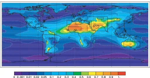
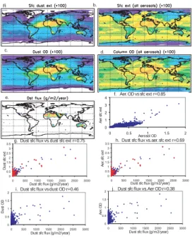
First we look at the ability of visibility data and satellite data to provide information about the spatial location of dust sources (Fig. 2). Notice that spatially, the maximum 20

in modeled dust sources are located in different places than the modelled maximum in dust aerosol optical depth or surface concentrations (these plots show monthly mean values for January of 1981, but any particular month or annual average will look similar). The surface concentrations visually appear more related to surface fluxes than optical depth visually. This is very clear in the scatter plots or the correlation coefficients, which 25

are shown for all land grid points in the model. The correlation coefficients between the spatial locations of dust surface fluxes and surface extinction or optical depth in model are 0.75 and 0.46, respectively. If we add in the complexity that in the real world we

(15)

ACPD

7, 3013–3071, 2007

Printer-friendly Version Interactive Discussion retrieve total aerosol surface extinction and optical depth (as opposed to just for dust)

and try to infer dust surface fluxes, these correlation coefficients drop to 0.69 and 0.38, corresponding to capturing 48% or 14%, respectively, of the spatial variability in dust surface fluxes, when we use surface extinction or optical depths, respectively. In the real world we only have visibility data at a limited number of stations, not globally as 5

we do in the model. If we sample the model output at these stations only, our cor-relation coefficient does not change substantially (0.73) In the real world, TOMS AAI does not sample optical depth, but an aerosol index which is linearly proportional to al-titude, making it likely to perform worse at detecting dust source fluxes than the model estimates here. The strength of sources is not well related to the frequency of emis-10

sions (Laurent et al., 2005), suggesting that sampling the number of times TOMS AAI is above a certain threshold (e.g. Prospero et al., 2002) is not necessarily a better way to obtain information about the sources. (Notice that for our visibility derived variable, VIS5, which is a frequency variable, does about as well as the EXT variable.) Thus, visibility derived variables (even at a limited number of stations) should theoretically do 15

a much better job of capturing the spatial variability in dust fluxes than satellite derived optical depth. Whether they practically do is based on their ability to capture regional scale aerosol fluctuations, which is examined in detail in Sect. 3.1.

Next we look at the ability of visibility derived variables or aerosol optical depth to capture temporal variability of dust source fluxes at individual gridboxes in the model. 20

These results (Figs. 3b and c) show a higher correlation between the monthly mean time series in modeled surface extinction and modelled dust surface fluxes than be-tween modelled AOD and modelled dust surface fluxes. Again, these results suggest that visibility derived variables will do a better job at capturing temporal variability in dust source fluxes than aerosol optical depths. This is only true in practice if the qual-25

ity of the visibility data in calculating surface extinction is similar to satellite retrieved column amount and has a similar spatial extent. Our analysis suggests that satel-lite retrieved aerosol optical depths are better than visibility derived surface extinction at capturing variability at AERONET sites (correlation coefficient of 0.66–0.7 against

(16)

ACPD

7, 3013–3071, 2007

Printer-friendly Version Interactive Discussion 0.47). Although previous studies have implicitly assumed that satellite derived

spa-tial and temporal variability are better than those derived from visibility measurements (e.g. Goudie and Middleton, 2001; Prospero et al., 2002) this analysis does not clearly support that assumption.

4 Visibility trends and correlations in dust regions 5

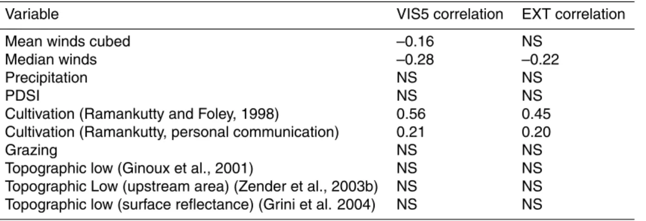
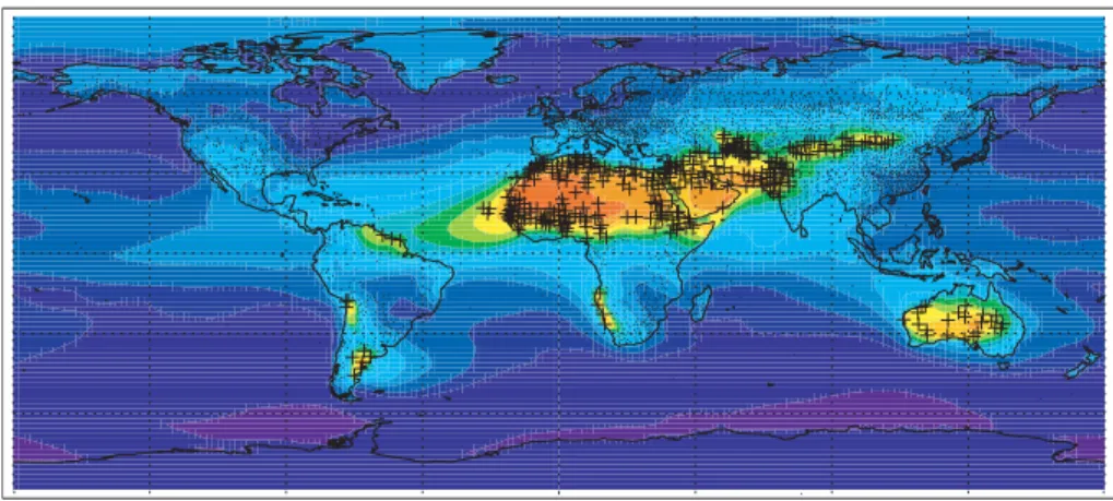
We focus on dust regions in this section. Since the analysis in Sect. 3 indicates that visibility best correlates with aerosol optical depth in dust dominated regions, we focus on the visibility-derived measures of dust here. Dust dominated regions are defined as those regions where dust contributes to at least 50% of the surface aerosol extinction in model simulations (Rasch et al., 2001). Figure 4 shows the locations of meteoro-10

logical stations with at least 30 years of data, and those within our dust dominated region. There are 357 stations from dust dominated regions included in the analysis of the visibility data. We analyze these stations grouped together by region, as well as individually.

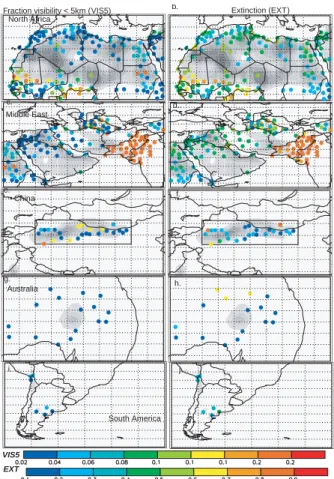
The mean fraction of observations when visibility is less than 5 km (VIS5) and mean 15

surface extinction (EXT) derived from visibility are shown for several different regions in Fig. 5 averaged over the period of 1974–2003. If we interpret this map as a proxy for dustiness, it gives us a very different view of where the dust sources are than what we get from TOMS AAI (e.g. Prospero et al., 2002). The Bodele basin does not appear to be the largest source of dust, as some have claimed (e.g. Prospero et al., 2002), 20

and looks quite moderate in this dataset. One area that stands out in this analysis as having a large number of events in the visibility data is the region around Pakistan and India, with low visibility (high VIS5 and EXT) also seen in parts of North Africa, the Middle East and China/Mongolia. We normally do not think of the region near Pakistan and northwestern India as being the largest dust source (e.g. Goudie and 25

Middleton, 2001; Prospero et al., 2002), and the reason this region has such high VIS5 and EXT values could be due to anthropogenic aerosols that may be stronger than

(17)

ACPD

7, 3013–3071, 2007

Printer-friendly Version Interactive Discussion our model predicts. On the other hand, Pakistan and northwestern India is generally

a highly populated region with an arid climate, and with some of the highest rates of reported desertification (Middleton and Thomas, 1997), so the visibility data could be correct. It is also possible that the visibility data are biased in that a given station could stop reporting data during dust events, biasing where the visibility data suggests 5

the most aerosols are located. There are no stations in North America where dust represents 50% of the surface extinction, and the stations in South Africa are too few to include for a conclusive analysis. The global distribution of EXT (extinction) and VIS5 (fraction of observations with visibility less than 5 km) is different, and this is one of the reasons we analyze both variables. They are equally good (or bad) measures 10

of aerosol optical depth, according to Sect. 3, and yet they are measuring aerosols differently – the number of extreme events (VIS5) compared to background visibility plus extreme events (EXT).

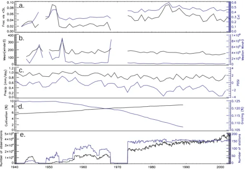
Next we look at each region individually; the bounds on the regional boxes used in the analysis below are shown globally in Fig. 1. For North Africa, we show a time se-15

ries of the average visibility, winds, precipitation, palmer drought severity index (PDSI) and human land use and grazing in Fig. 6. These values are averaged over the station locations (not over the entire region), to weight them in a manner similar to the visibility. Visibility derived variables (both EXT and VIS5) appear to vary substantially over the time series, even averaged over the whole of North Africa. We can see many visibility 20

events and high extinction during the 1970–1980s, associated with the Sahel drought and higher downwind dust concentrations (e.g. Prospero and Nees, 1986; Prospero and Lamb, 2003). After the 1980s, fractions of VIS5 values decrease by about 50% while the extinction values decreases more slowly. There is a peak of low visibility during the 1950s associated with high winds, but the data is quite spotty during the 25

1940–1960s. Thus it is not clear how robust these changes are, although they ap-pear at several different stations (not shown). Precipitation varies over this time period, dominated by the Sahel drought signal, and the Palmer drought severity index (PDSI) is highly correlated with precipitation. Cultivation tends to be increasing over this time

(18)

ACPD

7, 3013–3071, 2007

Printer-friendly Version Interactive Discussion period, while grazing is decreasing, especially after the 1950s. The poor temporal

res-olution of observations related to land use is obvious from this figure. Data availability is highly variable over the time period with most consistent observations only available after 1974. This is true in all of dust regions, and because of this we focus our analysis on the period 1974–2003.

5

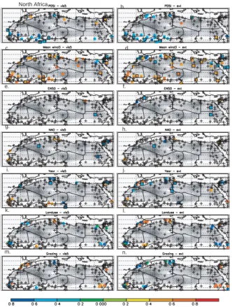
We focus next on correlations between these variables at specific stations from 1974–2003 in the North African region. For North Africa, the correlation coefficients between visibility derived variables and Palmer Drought Severity Index (PDSI), the av-erage of winds cubed, El Nino, NAO, year (indicates where there is a trend in the data), cropland and grazing are shown in Fig. 7. In these plots, reds indicate positive correla-10

tions, blues negative correlations, pluses indicate no statistically significant correlations (at 99 percentile significance), and boxes indicate that the correlations only exist be-tween that variable (see methods for how this is calculated) and the visibility derived variable. Notice that there are very few correlations which are captured by just one variable, indicating that interpreting the results of the correlation is not staightforward. 15

The strongest correlations are between the PDSI and mean cube of the winds and the VIS5 or EXT variable. We use mean cube of the winds because the strength of dust sources is usually proportional to winds cubed (e.g. Mahowald et al., 2005). This sug-gests that meteorology drives most of the temporal variability in North Africa, consistent with previous studies (e.g. Prospero and Nees, 1986; Mbourou et al., 1997; Prospero 20

and Lamb, 2003). The correlations at most stations between PDSI and visibility tend to be larger in magnitude than between precipitation, previous year’s precipitation or the previous year’s PDSI and visibility (not shown), consistent with drought severity being a better measure of soil moisture than precipitation alone. Thus, we focus on using the PDSI for the rest of the analyses. Surprisingly, there is little correlation be-25

tween ENSO or NAO and visibility in North Africa, unlike further downwind using other datasets (e.g. Moulin et al., 1997; Mahowald et al., 2003b). There are some statisti-cally significant trends in time (i.e. correlations with year) in the VIS5 and EXT, although they are opposite in sign in some cases along the Mediterranean coast of North Africa,

(19)

ACPD

7, 3013–3071, 2007

Printer-friendly Version Interactive Discussion indicating that the number of events is going up, but the background aerosol

concen-tration may be going down. If we do the correlation over 1940–2003, instead of just over the time period between 1974 and 2003, we obtain much stronger correlations between year and extinction and between land use and extinction along the Mediter-ranean coast of North Africa, perhaps associated with the difference in the amount of 5

data. Figure 8 shows the average time series in a region centered on Algeria (28 N to 3 N, 2 E to 15 E). This shows that there is little data before 1974, but that the data suggest episodes of high VIS5 and EXT during the 1950s and 1960s. There is a ten-dency for EXT to be higher later in the century, consistent with a correlation between EXT and year at individual stations (not just because of discontinuities in data records 10

at individual stations). There is also a positive correlation between EXT and cropland and a negative correlation between EXT and grazing (since cropland and grazing are almost linearly increasing and decreasing, respectively, over the 1940–1990s). Similar behaviour is seen for the average of all the stations in the W. Sahel (13 N to 22 N, 20 W to 15 E) time series (Fig. 9), with a peak in VIS5 and EXT in 1985 (during the Sahel 15

drought), with some high values of VIS5 and EXT in the 1940s and 1950s.

The time series for the Middle East region is shown in Fig. 10. Similar to North Africa, there tend to be many low visibility events in the beginning of the time record (1940–1960s), where there are few data. But during the 1974–2003 period, when the amount of data is more stable, there is not as much fluctuation in VIS5 or EXT, 20

although mean winds decrease. Correlation coefficients at each individual station over 1974 to 2003 (Fig. 11) suggest that meteorology is not as important as in North Africa, but that there are statistically significant temporal trends. There are also correlations between human activities (cropland or grazing) and dust in different parts of the Middle East. There are statistically significant decreases in Pakistan/India over 1974–2003. 25

If we look at correlations in Pakistsan/India over the longer time period (back to the 1940s) there are more stations with positive trends in VIS5 and EXT (not shown) and more statistically significant correlations with cropland and grazing (both positive and negative). For the sources in and around China (see Fig. 1 or Fig. 5c for region),

(20)

ACPD

7, 3013–3071, 2007

Printer-friendly Version Interactive Discussion we tend to see high VIS5 and EXT in the 1940s and 1950s, similar to other regions,

and a downward trend between 1974 and 2003 (Fig. 12). Correlations between VIS5 and EXT and other variables (Fig. 13) suggest that precipitation is not important for variability in visibility, but that winds are correlated with variability in visibility, similar to the results seen in other studies (e.g. Zhang et al., 2003; Sun et al., 2001; Zhao et 5

al., 2004; Liu et al., 2004). Our data do not show the increase in dustiness in 2000-2002 seen in Kurosaki and Mikami (2003), although our results are consistent with their conclusion that wind drives variability in dust events.

For Australia, there are fewer stations compared to the other regions previously dis-cussed, but again we see the low visibility in the 1950s, with less variability between 10

1974 and 2003 in the VIS5 and EXT data. There is an exception in the year 1986, which is anomalously high, especially for VIS5 (Fig. 14). Correlations at specific sta-tions (Fig. 15) suggest that PDSI has the strongest correlasta-tions with dust, but in a manner that is counterintuitive – the higher the water availability is, the more dust. This makes some sense if the increasing water makes the soil more erodible because 15

the water brings more erodible sediment into the dry fluvial channels and lake beds (e.g. Okin and Reheis, 2002; Mahowald et al., 2003a; Zender and Kwon, 2005 . There are downward trends in VIS5 and EXT over the 1974–2003 time periods at some sta-tions (similar results are seen for Fig. 15 when the whole time period is considered). There are 2 (out of 16) stations with statistically significant correlations between VIS5 20

and ENSO, but these significant correlations are not matched between EXT and ENSO. (*This is in contrast to the correlation between El Nino and precipitation in many regions of Australia, although no necessarily across the dust region (Dai et al., 1998).

In South America, there are 7 stations with data for part of the time period. Again there are low visibilities at the first part of the time series, and then flatter visibility 25

trends for the rest of the time series (Fig. 16). There are few correlations between the station data and other variables (Fig. 17). Some stations indicate that wind speeds are anti-correlated with VIS5 and EXT (which may indicate that these stations are not dust dominated and should be ignored), and there are some correlations between year,

(21)

ACPD

7, 3013–3071, 2007

Printer-friendly Version Interactive Discussion cropland, grazing and precipitation, but no large scale patterns. Only one station has a

correlation between ENSO and EXT.

There are a couple of regions where our model does not predict the surface extinction to be dominated by dust, but where dust emissions may be important. We consider them briefly here, including all stations with more than 30 years of data. First we look 5

at the Southwestern U.S. region (e.g. Prospero et al., 2001) (Fig. 19 shows the region). A time series plot shows that both VIS5 and EXT have been roughly increasing since the 1940s, with a lot of variability (Fig. 18). For this region, the data are more regularly available prior to 1974 than in previous regions, so we show correlations from 1940 to 2003 (Fig. 19). There are statistically significant correlations between most of the 10

variables and VIS5 or EXT. Winds and antecedent PDSI are sometimes anti-correlated with VIS5, which is not intuitive. Increases in precipitation may bring in more easily erodible soil (Mahowald et al., 2003a; Okin and Reheis, 2002), but lower winds seem unlikely to contribute to greater dust sources. Both the results of the correlations, as well as the fact that these regions are not generally dominated by dust make the 15

interpretation of these results difficult, and are consistent with the results of the model suggesting that visibility in this region is not dominated by dust.

The Aral Sea area is another region which is thought to have a great deal of dust (e.g. Prospero et al., 2001), although our model does not predict dust as the dominant source of surface extinction. VIS5 and EXT tended to be high during the 1950s, and 20

are lower now (Fig. 20). Similarly, winds were higher in the 1950s than today. These might be indications that the data quality or location of the measurement devices have changed, or it could be an indication that there are real changes in the conditions in the Aral Sea. Similar to North America, the amount of data is relatively stable over the whole period of data (1940–2003), so we show correlations over the whole period 25

(Fig. 21). There are strong correlations between wind speed cubed and VIS5 and EXT as well as between grazing and VIS5 or EXT. There are anti-correlations between VIS5 and EXT and cropland and year. Studies have shown that Aral Sea levels have dropped dramatically, and that the area of the Sea has been reduced by about 80% in

(22)

ACPD

7, 3013–3071, 2007

Printer-friendly Version Interactive Discussion recent decades. There have only been anecdotal studies of the changes in dustiness

of the region (e.g. Smith et al., 1999). The visibility-based data does not support a decrease in visibility since the 1940s. This could be because of shifts in winds as the lake has dried up.

If we consider the average of all 357 stations in dusty regions (Fig. 22), we see that 5

the 1940s and 1950s were periods with relatively high VIS5 and EXT. These were more windy periods, although there is also more variability in winds. It is interesting that there was higher VIS5 and EXT during this period, but it raises a question about the data. It could be that during this period, there were more dirt roads close to the meteorological stations, and this caused lower visibility. This was a period of rapid changes due to 10

the World War and technological development. There may also have been an increase in soil conservation efforts in cultivated areas after this time period. But these results could also be an indication that the measurement techniques are not consistent across our entire time period. Overall, the appearance of a peak in both EXT and VIS5 at the beginning of our time series, when the data were relatively sparse, appears suspicious. 15

Thus, we may want to readdress previous studies which have suggested the 1950s were dustier in China than current (Zijiang and Guocai, 2003), as an example, and see if there are independent datasets which allow us to check that this result is not because of biases in the data collection method. On the other hand, it is possible that the 1940s and 1950s were a much dustier time period in all dust regions globally. Over 20

the whole time period, there is no statistically significant trend in EXT or VIS5 for all regions taken together. For some regions (China, Middle East or South America) there are statistically significant trends with time in the visibility derived variables over the whole time period or 1974–2003 (see Table 3).

Another way to analyze the same data is to look at correlations between VIS5 and 25

EXT and other variables not over time, but in space across the stations. If we look at the spatial correlations across all regions using the means over all years (or over 1974–2003, the results do not change qualitatively), we can look at some different hypotheses about drivers of dust variability spatially. For the correlations between

(23)

ACPD

7, 3013–3071, 2007

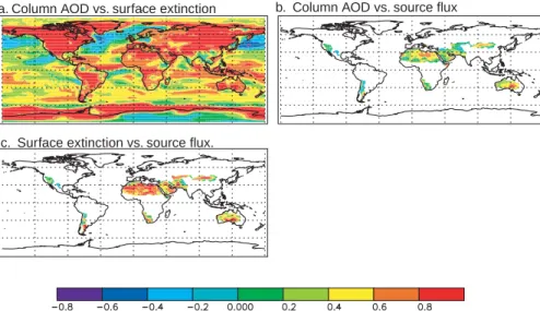
Printer-friendly Version Interactive Discussion ibility parameters and topographic lows we use three representations: the preferential

source distribution of Ginoux et al. (2001), the dust source used in the NCAR Com-munity Atmospheric Model (Mahowald et al., 2006) (which is based on the Zender et al. (2003b) geomorphic soil erodibility factor which calculates upstream area and satel-lite derived vegetation, Bonan et al., 2002), or the surface reflectance-based sources 5

of Grini and Zender (2004). In addition to the mean cropland extent from Ramankutty and Foley (1998) used in the main part of the study, we use a new cropland dataset being developed for 2000 (Ramankutty, personal communication). Table 4 shows the results of this analysis over the 357 stations in dust dominated regions. These results suggest that cultivation is the best determinant of spatial variability in dustiness, not 10

wind speed or whether there are topographic lows nearby. This is in contrast to a pre-vious work based on fraction of events where visibility is less than 1 km and a slightly different topographic low dataset (Engelstaedter, et al., 2003). The correlation coeffi-cients between cropland extent (Ramankutty and Foley, 1998) and VIS5 and EXT are 0.55 and 0.45 respectively, consistent with cultivation being associated with 20–30% 15

of the dustiness seen in the visibility record. We obtain similar results if we use the more recent dataset developed for the year 2000 (Ramankutty, in prep.), although this correlation is sensitive to the resolution of the cropland data. At too high of a res-olution (5 min) the correlation decreases, probably because croplands which may be associated with dust sources are not located in the same 5 min grid box as our sta-20

tions, but are located within the 100 km grid size. In addition, we can analyze several variables at the same time and see if more variability is captured. If we include winds cubed, PDSI, croplands, grazing and topographic lows, slightly higher correlations co-efficients are found than for any individual process (0.58 and 0.50 vs. 0.55 and 0.45 for VIS5 and EXT, respectively), and these results also suggest that cultivation is the 25

most reliable variable for predicting visibility distributions. This result is consistent with the view of visibility that we obtain from Fig. 5, where the lowest visibility (i.e. highest VIS5 and EXT) is observed in Pakistan and northwestern India, where cultivation in an arid region may be contributing to high rates of desertification (Middleton and Thomas,

(24)

ACPD

7, 3013–3071, 2007

Printer-friendly Version Interactive Discussion 1997).

5 Summary and conclusions

This study focuses on using visibility data from surface meteorological stations as an indicator of dust variability, and specifically dust source variability. Because the quanti-tative nature of visibility data is not well established, we first evaluate the utility visibility 5

data for our purposes. Our goal is to look at long term variability, so we use the monthly mean AERONET aerosol optical depth (AOD) at the 33 stations with more than 3 years of data. While AERONET data is high quality, it is not available as spatially or tempo-rally extensively as the visibility data.

For each AERONET station, the monthly mean AOD values are compared to visibility 10

derived variables at the closest two meteorological stations. At many stations there are no statistically significant correlations between the column aerosol optical depth and the visibility derived variables, although theoretical calculations suggest there should be. Overall, for the surface extinction and monthly fraction of events with<5 km

visi-bility, the correlations are 0.25 and 0.33, respectively, implying that between 4 and 9% 15

of the variability in aerosol optical depth is captured by the visibility data. If we focus on stations that are predicted to be dominated by dust based on model calculations, we obtain overall correlations for extinction and fraction of observations with a visibility

<5 km of 0.47 and 0.46, respectively. These results suggest that about 22% of the

variability in the optical depths is captured in the visibility derived variables. We tested 20

several different visibility derived variables, and results suggest that the fraction of ob-servations with a visibility less than 1 km is less well correlated with aerosol optical depth than either fraction of visibility less than 5 km (VIS5) or averaged surface extinc-tion (EXT; related to 1/visibility), so we used those variables for most of the analyses in this paper. This suggests that previous papers emphasizing the fraction of observa-25

tions with visibility less than 1 km may not be looking at the best parameter to represent dustiness (e.g. Engelstaedter et al., 2003).

(25)

ACPD

7, 3013–3071, 2007

Printer-friendly Version Interactive Discussion Similar correlation analyses using the TOMS AAI and TOMS AOD data suggest that

they are able to capture about 45–49% of the variability in the AERONET optical depth data over dusty regions (correlation coefficients of 0.67 and 0.7). Note that the TOMS AOD only has a correlation coefficient of 0.23 over all AERONET stations, suggesting that it is not a robust measure of temporally and spatial variability in aerosol optical 5

depth in non-dusty regions, even ignoring problems in satellite drift outside the 1984– 1990 period.

For this study, and many previous studies, we use measures of dust AOD or surface extinction to infer the location and temporal variability of dust source surface fluxes, since we cannot directly measure dust source surface fluxes globally. Using models we 10

can better understand which variables best represent the spatial and temporal variabil-ity in dust source surface fluxes. Our calculations show that surface extinction should be much better related to source surface fluxes of dust than column amount (correlation coefficient of 0.73 vs. 0.38, equals 36% vs. 10% of variability, respectively). Thus, it is unclear whether satellite aerosol optical depth or visibility derived variability best gives 15

information about variability in dust sources (either spatial or temporal). Some studies assume that TOMS AAI represents the long-range transported dust (e.g. Prospero et al., 2002). Because TOMS AAI is linearly proportional to the height of the dust, this is probably true (Torres et al., 1998; Mahowald and Dufresne, 2004). However, this also makes TOMS AAI less appropriate for studying spatial or temporal variability in dust 20

source fluxes. The visibility derived-proxies represent regional aerosols to the extent that they correlate with the AERONET AODs, and thus represent dust that has been transported somewhere from the kilometer to the hundreds of kilometers scale. The analysis here suggests that visibility data and TOMS AAI or TOMS AOD may be equiv-alently good (or bad) at representing the spatial and temporal variability in surface dust 25

fluxes. More work on determining better ways to determine the location of dust source areas is vital, since the two main datasets we have to address dust sources (satel-lite optical depths or visibility data) show different results. We examined the temporal trends in VIS5 and EXT in regions dominated by dust, where the visibility derived

(26)

vari-ACPD

7, 3013–3071, 2007

Printer-friendly Version Interactive Discussion ables are able to capture over 20% of the variability in aerosol optical depth measured

by AERONET. Although meteorological station data are available from 1900 to 2003, in dusty regions there are only data after 1940 in our dataset. The data record prior to 1974 is not consistent, forcing us to limit our analysis of ‘long’ term trends to the last 30 years. This is disappointing, since we had hoped to extend the satellite record signifi-5

cantly into the pre-1980s period. This implies we are missing any processes occurring prior to the 1970s.

Analysis of the temporal variability in VIS5 and EXT shows that there are maxima in the 1940s and 1950s throughout most of the dust regions. It is unclear whether these maxima occur because this was a dustier time period, or because of changes in 10

measurement methods, scarceness of the data during this period, or an increase in dirt roads (which were later paved) or changes in farming practices (contour plowing, no-till agriculture and crop land intensification). In order to better understand what happened in the 1940s to 1950s, we should try to find independent datasets before concluding that it was a dustier period.

15

There are a relatively stable number of observations after 1974 in the dataset over dusty regions, so we conducted most of our correlation analyses between individual station time series of VIS5 or EXT and other variables during the period 1974–2003. For analysis we present simple correlation coefficients, but rank correlations show qual-itatively similar results. However, in many cases, there are multiple variables which 20

correlate with the visibility derived proxies, making it more difficult to interpret the re-sults. We focus on results that are regionally coherent. The high correlation coefficients between annually averaged PDSI and both VIS5 and EXT are consistent with precipi-tation being very important in the Sahel region of North Africa and the Mediterranean coast of North Africa. High correlations between winds and VIS5 or EXT in China are 25

consistent with winds driving much of the variability of dustiness in China. In other re-gions, the correlation coefficients are not statistically significant on a regional basis. In no region are there large numbers of strong correlations between either NAO or ENSO and visibility, unlike what is seen farther downwind (e.g. Moulin et al., 1997; Mahowald

(27)

ACPD

7, 3013–3071, 2007

Printer-friendly Version Interactive Discussion et al., 2003b; Prospero and Lamb, 2003). Temporally, correlations between human

cultivation or grazing and visibility derived variables are not seen over large regions in our datasets, perhaps due to the poor temporal quality of the cultivation and grazing datasets.

There are regions with statistically significant trends with time in VIS5 or EXT for the 5

period 1974–2003 (seen as a correlation between year and these variables). Upward trends with time are seen regionally in parts of North Africa, especially in EXT, corre-lated with lower precipitation. Downward trends are seen in regionally broader areas, including parts of Central Asia and China. Looking at the average across all 357 sta-tions in dusty regions, there is no statistically significant trend in VIS5 or EXT. Note that 10

analyses of North America and the region close to Aral Sea (while more uncertain be-cause these regions’ visibility is not dominated by mineral aerosols) suggest that EXT and VIS5 are decreasing in these regions.

We get a different picture of the important processes if we look spatially across sta-tions instead of at individual stasta-tions over time. The hypothesis that dry lake beds are 15

dust sources is not supported, since there is no significant correlation between mean VIS5 or EXT in our data and three measures of the topographic lows (to the extent that topographic lows represent dry lakebeds). Instead the most consistent correlations are between VIS5 and EXT and cultivation across all regions, with correlation coeffi-cients suggesting that approximately 30% of the spatial distribution in the dustiness in 20

the stations is associated with cultivation (note this does not mean that the cultivation source of dust is 30% of the dust flux, because of the statistics used here). Much of this cultivation related dustiness appears to be in the Pakistan/India region (see Fig. 5). This may indicate that the results here may be sensitive to the quality of this data as a reflection of dust sources. The hypothesis that most dust comes from topographic 25

lows is supported from the TOMS AAI data and other geomorphic data (e.g. Goudie and Middleton, 2001; Prospero et al., 2002). However, the visibility data do not support that hypothesis. Which dataset should we believe? According to the analysis here, it is likely that the visibility derived data used here or TOMS AAI or TOMS AOD are

(28)

ACPD

7, 3013–3071, 2007

Printer-friendly Version Interactive Discussion equally good (or bad) at inferring the spatial and temporal variability of dust surface

fluxes. In addition, the TOMS AAI retrieval method is biased to show higher values in dry topographic lows in desert regions than in other nearby regions (Mahowald and Dufresne, 2004). Thus, this paper suggests we need to re-examine the hypothesis that topographic lows are the dominant source of dust. Using datasets that represent the 5

vegetation, land use, and underlying soils and landforms would provide a more physi-cal basis from which to understand dust sources (e.g. Ballantine et al., 2005) Because of the known biases of the TOMS AAI specifically, and the poor correlation of AOD with dust surface fluxes, other datasets should be used to improve our understanding of dust sources.

10

Any conclusions about what drives variability in desert dust sources based on visi-bility data must include a caveat, because of the question about the quality of the data. Comparisons suggest that the visibility data only capture about 22% of the variability in aerosol optical depth, and thus may be describing only about 20% of our dust source variability (assuming that our data are Gaussian, which they are not). However, visibility 15

datasets are more extensive in time and space than our other datasets, and may be as good as datasets from satellites at looking at surface emissions of dust (e.g. TOMS AAI or T OMS AOD). The visibility data sets here suggest very little global trend in dusti-ness for the period of 1974–2003. One of the major problems with predicting changes in desert dust sources and loading is de-convolving the relative roles of climate change, 20

carbon dioxide fertilization and land use in impacting dust mobilization. The temporal analysis performed in this study suggests that climate variability and change (through wind changes, and the impact of changes in soil moisture from precipitation and sur-face temperature changes) and potentially carbon dioxide fertilization, and not human land use practices, drive temporal changes in dust sources between 1974 and 2003 25

in some regions. However, spatial analysis of dustiness seen in the visibility record is consistent with a large fraction of the dustiness being associated with human land use, especially in Pakistan and India. Therefore this analysis suggests that land use perturbations may control where a significant portion of the dust sources are, but that