Publisher’s version / Version de l'éditeur:
Vous avez des questions? Nous pouvons vous aider. Pour communiquer directement avec un auteur, consultez la
première page de la revue dans laquelle son article a été publié afin de trouver ses coordonnées. Si vous n’arrivez pas à les repérer, communiquez avec nous à [email protected].
Questions? Contact the NRC Publications Archive team at
[email protected]. If you wish to email the authors directly, please see the first page of the publication for their contact information.
https://publications-cnrc.canada.ca/fra/droits
L’accès à ce site Web et l’utilisation de son contenu sont assujettis aux conditions présentées dans le site LISEZ CES CONDITIONS ATTENTIVEMENT AVANT D’UTILISER CE SITE WEB.
Internal Report (National Research Council of Canada. Institute for Research in
Construction), 2006-03-01
READ THESE TERMS AND CONDITIONS CAREFULLY BEFORE USING THIS WEBSITE. https://nrc-publications.canada.ca/eng/copyright
NRC Publications Archive Record / Notice des Archives des publications du CNRC :
https://nrc-publications.canada.ca/eng/view/object/?id=e2964d16-22af-46a2-b162-005f828dfa18
https://publications-cnrc.canada.ca/fra/voir/objet/?id=e2964d16-22af-46a2-b162-005f828dfa18
Archives des publications du CNRC
For the publisher’s version, please access the DOI link below./ Pour consulter la version de l’éditeur, utilisez le lien DOI ci-dessous.
https://doi.org/10.4224/20377138
Access and use of this website and the material on it are subject to the Terms and Conditions set forth at
Resilient modulus and permanent deformation test for unbound
materials
Re silie nt M odulus a nd Pe r m a ne nt
De for m a t ion Te st for U nbound M a t e ria ls
I R C - I R - 8 7 2
A b u s h o g l i n , F . ; K h o g a l i , W .
DOCUMENT TITLE: REVISION #2
Institute for Research in
Construction
Resilient Modulus and Permanent Deformation Test
for Unbound Materials
DRAFT # 1 PROGRAM:
IRC
EFFECTIVE DATE: MARCH 03, 2006APPROVALS
The following approvals have been obtained prior to issuance of this work instruction.
Fathi Abushoglin
February
06,
2006
Author
Date
Walaa Khogali
February
06,
2006
Co-Author
Date
ElHussein H. Mohamed
February
07,
2006
Reviewed
Date
Kleiner, Yehuda March
01,
2006
Program
Director
Date
James Crawford
March
03,
2006
Quality
Assurance
Manager
Date
FILE PATH:
Iso9000 on ‘Irc-public':\Urban Infrastructure
Rehabilitation\Work Instructions\Urban Roads
THIS DOCUMENT IS NOT CONTROLLED, UNLESS
PROGRAM:
IRC
EFFECTIVE DATE: MARCH 03, 2006
Contents
Part I: Sample Preparation and Test Protocol
1. Scope
2. Significance and Use
3. Definition of Terms
4. Apparatus
5. AASHTO
Documentation
6. Sample Preparation Protocol
7. Sample Setup and Testing
Part II: Data Reduction and Analysis of Test Results
1. Calculation of Mechanical Properties
2. NRC
Macro
FILE PATH:
Iso9000 on ‘Irc-public':\Urban Infrastructure
Rehabilitation\Work Instructions\Urban Roads
THIS DOCUMENT IS NOT CONTROLLED, UNLESS
Institute for Research in
Construction
DOCUMENT TITLE:
Resilient Modulus and Permanent Deformation Test
for Unbound Materials
REVISION #2 DRAFT # 1 PROGRAM:
IRC
EFFECTIVE DATE: MARCH 03, 2006Part I
Sample Preparation and Test Protocol
FILE PATH:
Iso9000 on ‘Irc-public':\Urban Infrastructure
Rehabilitation\Work Instructions\Urban Roads
THIS DOCUMENT IS NOT CONTROLLED, UNLESS
PROGRAM:
IRC
EFFECTIVE DATE: MARCH 03, 2006
1. Scope
This manual describes procedures for preparing and testing unbound materials, including cohesive and granular materials, for the determination of the resilient modulus (Mr) and permanent deformation response. Samples are to be
tested under conditions prevailing in the road layer in which the evaluated material is located. These conditions include density and moisture state as well as the level of traffic-induced stress estimated for the layer under consideration. The methods described here are applicable to undisturbed samples obtained from the field as well as samples prepared in the laboratory using appropriate compaction procedures.
2. Significance and use
The resilient modulus – permanent deformation test provides a set of mechanistic parameters that uniquely describe the material response to traffic loading under prevailing physical conditions. The test setup and sample preparation techniques described in this manual may also be used to obtain the Poisson’s ratio. These parameters are used as input to the design and analysis of road structures.
The test results may also be used to establish a material selection criterion based on its ability to perform effectively in terms of permanent deformation sustained.
3. Definition of terms
3.1 Symbols used
σ1 is the total axial stress (major principal stress)
σ3 is the applied confining pressure (minor principal stress, and σ2 = σ3)
σd = σ1 - σ3 is the deviator repetitive stress
εT is the total axial strain due to σd
εp is the permanent (non-recoverable) axial strain due to σd
εr is the resilient axial strain due to σd
εT = εr + εp
Mr = σd / εr is the resilient modulus
PD is the permanent deformation (%)
3.2 Terminology
Load duration is the time interval the sample is subjected to a deviator stress. Cycle duration is the time interval between successive applications of a deviator stress (cycle duration = load duration + rest period).
For the purposes of this manual, materials will be designated granular or cohesive following AASHTO Designation T292-91. Other materials that can be tested using procedures set in this manual include flowable fills.
4. Apparatus
Figure 1 displays the main components of the resilient modulus – permanent deformation (Mr − PD) Test System.
Following is a description of each of these components.
FILE PATH:
Iso9000 on ‘Irc-public':\Urban Infrastructure
Rehabilitation\Work Instructions\Urban Roads
THIS DOCUMENT IS NOT CONTROLLED, UNLESS
DOCUMENT TITLE: REVISION #2
Institute for Research in
Construction
Resilient Modulus and Permanent Deformation Test
for Unbound Materials
DRAFT # 1 PROGRAM:
IRC
EFFECTIVE DATE: MARCH 03, 2006Triaxial
Chamber
Pressure
Manifold
Hydraulic
Actuator
Loading Frame
Data Acquisition System Test Sample
Figure 1. Components of the
Mr − PDtest system
4.1 Triaxial Pressure Chamber – The chamber is used to house the test specimen and to provide the environment
for the application of the confining pressure. Air is used as the confining fluid for all tests performed on granular and cohesive materials. Two triaxial chambers of different sizes are used for granular and cohesive material specimens. A large cell, which can accommodate 152.4 mm (6 in.) diameter samples, is used for testing granular specimens while a smaller cell, capable of accommodating 76.2 mm (3 in.) diameter samples, is used for cohesive specimens. Images showing different components of the triaxial cells are displayed in Figures 2 and 3. Schematic diagrams depicting details of the configuration of the two cells are included in Appendix A (Figures A1 and A2).
4.2 Loading Frame – The axial repetitive deviator stress, σd, is provided by means of a closed loop hydraulic
system capable of producing various load durations and cycle durations. A haversine wave of load duration of 0.1-second and cycle duration of 1.0-second is recommended for testing both granular and cohesive materials. A typical load cycle is shown in Figure 4.
FILE PATH:
Iso9000 on ‘Irc-public':\Urban Infrastructure
Rehabilitation\Work Instructions\Urban Roads
THIS DOCUMENT IS NOT CONTROLLED, UNLESS
PROGRAM:
IRC
EFFECTIVE DATE: MARCH 03, 2006
Figure 2. Triaxial Pressure Chamber (152.4 mm; 6 in.-cell configuration)
Figure 3. Triaxial pressure chamber (76.2 mm; 3 in.- cell configuration)
Load per cycle-250 -200 -150 -100 -50 0 0 0.1 0.2 0.3 0.4 0.5 0.6 0.7 0.8 0.9 1 1.1 Duration (sec) Loa d ( lb) a b d c
Figure 4. Typical axial load cycle
4.3 Axial Deformation Measuring Equipment – Two linear variable differential transformers (LVDT) are used to
monitor axial deformation in the specimen. Specifications for the LVDTs are given in Table 1. Both LVDTs are mounted internally onto the sample. The LVDTs are mounted 180 degrees diametrically opposite about the specimen’s axis (see Figures A1 and A2).
FILE PATH:
Iso9000 on ‘Irc-public':\Urban Infrastructure
Rehabilitation\Work Instructions\Urban Roads
THIS DOCUMENT IS NOT CONTROLLED, UNLESS
DOCUMENT TITLE: REVISION #2
Institute for Research in
Construction
Resilient Modulus and Permanent Deformation Test
for Unbound Materials
DRAFT # 1
PROGRAM:
IRC
EFFECTIVE DATE: MARCH 03, 2006
Table 1. Specifications for LVDTs and load cell
Characteristic Load Cell LVDT Minimum sensitivity, mm/v 2 0.2 mv/0.25 mm/v (AC LVDT) Non-linearity, percent FS 0.25 0.25 Hysteresis, percent FS 0.25 0.0 Repeatability, percent FS 0.10 0.01 Thermal effects on zero shift or sensitivity, percent FS/°C 0.005 mm (0.025 in.) Maximum deflection at full rated load, mm (in.) 0.125 mm (0.005 in.) Maximum capacity/ Minimum range Specimen 71 mm (2.8 in.) Specimen 152 mm (6.0 in.) 135 kg (300 lb) 680 kg (1500 lb) ± 6.25 mm (0.25 in.) ± 13.0 mm (0.50 in.)
4.4 Axial Load Measuring Device – An electronic load cell is used to monitor the repeated load applied by the
hydraulic loading system. The load cell is mounted internally on the top of the test specimen. Specifications for the load cell are given in Table 1.
4.5 Confining Pressure Measuring Device and Regulator – A pressure manifold should be used to regulate the
air pressure applied to the test specimen. A pressure transducer, mounted externally to the triaxial chamber, measures the confining pressure.
4.6 Data Acquisition – The Mr − PD Test System should be operated and controlled by a PC computer and an
advanced controller (such as the MTS TestStar IIm) capable of providing a high data-sampling rate. The data acquisition system should have four channels to collect the repetitive axial load, the two LVDT signals and the confining pressure data. The data may be analyzed using a spreadsheet (a Microsoft Excel macro was developed at NRC. Electronic copy will be provided as an attachment to this manual).
4.7 Calibration – Calibration of LVDTs, internal load cell, and pressure transducer should be performed at
regular intervals (every six weeks if tests are conducted daily or at longer intervals if tests are conducted occasionally). Hard copies of calibration sheets should be produced and kept for future reference. Figures 5 and 6 show examples of calibration data for one LVDT and the load cell.
FILE PATH:
Iso9000 on ‘Irc-public':\Urban Infrastructure
Rehabilitation\Work Instructions\Urban Roads
THIS DOCUMENT IS NOT CONTROLLED, UNLESS
PROGRAM:
IRC
EFFECTIVE DATE: MARCH 03, 2006 MTS load cell (S/N 63021) y = 0.9997x + 0.4834 R2 = 1 -3500 -3000 -2500 -2000 -1500 -1000 -500 0 500 -4000 -3000 -2000 -1000 0 Applied load (lbs) M T S r eadi ng ( lbs)Figure 5. Calibration sheet for a load cell
Actuator LVDT (+/- 3" stroke) y = 1.0008x + 76.168 R2 = 1 -20 0 20 40 60 80 100 120 140 160 180 -100.000 -50.000 0.000 50.000 100.000 MTS reading (mm) D ial r eadi ng ( m m )
Figure 6. Calibration sheet for an LVDT
4.8 Specimen Preparation Equipment – Equipment needed for preparing samples includes:
4.8.1 Shovels and containers for fractionating and reducing samples of aggregate to testing size (Following AASHTO T248-95).
4.8.2 Equipment for extraction and trimming specimens from undisturbed samples.
4.8.3 Rubber membranes – the rubber membrane used to encase the test specimen should provide proper protection against leakage. Membranes should be carefully inspected prior to use, and if any flaws are detected, the membrane should be discarded. For the membrane to provide minimum restraint to the specimen, its unstretched diameter should be between 90% and 95% of that of the specimen. Also the membrane thickness should not exceed 1% of the diameter of the specimen. Membranes typically used for cohesive materials are 76.2 mm (3
in.)
in diameter while those used for granular materials are 152.4 mm (6in.)
in diameter. Since granular materials contain angular particles, two membranes should be used with specimens made out of this type of material.4.8.4 Equipment for compaction of granular materials – a mechanical vibrator capable of providing 2100 blows/minute is recommended for compaction of granular materials. The following accessories (shown in Figures 7 – 11) are required for sample preparation:
• Spilt mold (152.4 mm; 6 in. diameter by 304.8 mm; 12 in. height)
• Cylindrical metal adapters (eight units with different dimensions as illustrated in Figures 7 and 8), • 152.4 mm (6 in.) diameter spacer with handle
FILE PATH:
Iso9000 on ‘Irc-public':\Urban Infrastructure
Rehabilitation\Work Instructions\Urban Roads
THIS DOCUMENT IS NOT CONTROLLED, UNLESS
DOCUMENT TITLE: REVISION #2
Institute for Research in
Construction
Resilient Modulus and Permanent Deformation Test
for Unbound Materials
DRAFT # 1
RAM:
IRC
PROG EFFECTIVE DATE:
MARCH 03, 2006
• Sample carrying assembly for transporting prepared specimens.
8.937″
H = Variable
6″
Adapter H
1
11.93″
2
10.51″
3
8.94″
4
7.44″
5
5.945″
6
4.626″
7
2.913″
8
1.22″
Figure 7. Adapters used for compaction of granular specimens (1 in. = 25.4 mm)
4.8.5 Equipment for static compaction of cohesive materials – the list includes: • Compaction mold (76.2 mm; 3
in.
diameter by 152.4 mm; 6in.
height)• Risers – these are metal cylinders with a 70 mm (2.756
in.)
external diameter and variable heights (as illustrated in Figure 13)
• Loading ram
• Extrusion ram, and an extrusion mold.
The equipment and accessories described herein are
s
hown in Figures 12, 13 and A3 of Appendix A.FILE PATH:
Iso9000 on ‘Irc-public':\Urban Infrastructure
Rehabilitation\Work Instructions\Urban Roads
THIS DOCUMENT IS NOT CONTROLLED, UNLESS
PROGRAM:
IRC
EFFECTIVE DATE: MARCH 03, 2006
Figure 8. Split mold and vibrator for preparation of granular specimens
Figure 9. Cylindrical adapters used for compaction of granular specimens
4.8.6 Miscellaneous apparatus – This includes calipers, micrometer gauge, steel rulers, pickers, rubber O-rings, vacuum source with bubble chamber and regulator, porous stones, scales, moisture content containers, Hobart mechanical mixer, an oven, and a balance with measurement accuracy of 1 g.
Figure 10. 152.4 mm (6 in.)–Diameter spacer
FILE PATH:
Iso9000 on ‘Irc-public':\Urban Infrastructure
Rehabilitation\Work Instructions\Urban Roads
THIS DOCUMENT IS NOT CONTROLLED, UNLESS
THE ABOVE QA SIGNATURE IS IN RED INK.
Page 10 OF
DOCUMENT TITLE: REVISION #2
Institute for Research in
Construction
Resilient Modulus and Permanent Deformation Test
for Unbound Materials
DRAFT # 1
PROGRAM:
IRC
EFFECTIVE DATE: MARCH 03, 2006
Figure 11. Sample carrying assembly
Figure 12. Equipment for preparation of cohesive specimens
5. AASHTO documentation
The following AASHTO documentations are to be used in reference to procedures adopted in this manual. M145 The Classification of Soils and Soil-Aggregate Mixtures for Highway Construction Purposes T11 Materials Finer Than 75 µm (No. 200) Sieve in Mineral Aggregates by Washing
T88 Particle Size Analysis of Soils
T180 Moisture-Density Relations of Soils Using a 4.54 kg (10 lbs) Rammer and a 457 mm (18 in.) Drop (Modified Proctor)
T100 Specific Gravity of Soils
T234 Unconsolidated, Un-drained Compressive Strength of Cohesive Soils in Triaxial Compression T248 Reducing Samples of Aggregates to Testing Size
T265 Laboratory Determination of Moisture Content of Soils
T292-91 Resilient Modulus of Subgrade Soils and Untreated Base/Subbase Materials
FILE PATH:
Iso9000 on ‘Irc-public':\Urban Infrastructure
Rehabilitation\Work Instructions\Urban Roads
THIS DOCUMENT IS NOT CONTROLLED, UNLESS
THE ABOVE QA SIGNATURE IS IN RED INK.
Page 11 OF
PROGRAM:
IRC
EFFECTIVE DATE: MARCH 03, 2006
6. Sample preparation protocol
6.1 Cohesive materials
The following procedure describes the preparation of cohesive specimens in the laboratory using disturbed material. The recommended test specimen size to be used is 71.1 mm (2.8 in.) diameter by 142.3 mm (5.6
in.)
height.6.1.1 Place material retrieved from the field in a large tray and dry in the oven for 24 hours at 110°C (230°F). 6.1.2 Remove tray from the oven and let it stand for half an hour for the material to cool down to room
temperature.
6.1.3 While the material is cooling, produce a hard copy of the sample preparation sheet shown in Figure A4 in Appendix A. Start filling this sheet with the introductory information identified as Data Block #1. The MTS specimen # refers to the name of the PC file used to store test data results.
6.1.4 Enter the maximum dry density and moisture content conditions that the specimen will be tested at using appropriate cells within Data Block #2. At this stage, also enter the dimensions of the compaction mold and number of compaction layers (refer to Data Block #2 in Figure A4).
6.1.5 Measure the thickness of two 76.2 mm (3 in.)-diameter porous stones then soak them in water until the time they are needed to be used. Record the weight of the saturated porous stones. Enter the information obtained in their respective cells within Data Block #3 in Figure A4.
6.1.6 Weigh the rubber membrane and O-rings that will be used during sample preparation. Record these measurements in their appropriate cells within Data Block #3.
6.1.7 Wearing a dust mask, grind the dry material obtained from step 6.1.2 with a mortar and pestle. Continue the grinding process until enough material is produced. The amount of material needed should be equal to the “weight of dry material” shown in Data Block #2 plus 250 g (0.55 lbs). This amount should be sufficient to produce the required test specimen with a remaining surplus that can be used for initial moisture content determination (i.e. “Before Mr test”, shown in Data Block #4 in Figure A4.)
6.1.8 Mix the dry material obtained from step 6.1.7 with water (equal to the amount shown in cell “Total weight of water in mix” in Data Block #3). Continue mixing until water is thoroughly and uniformly distributed within the material. Cover the mixing bowl to avoid moisture loss.
6.1.9 Scoop out six portions from the mass of the wet soil mix such that each portion weighs approximately the amount indicated in the Excel sheet cell designated as “weight of soil mix per layer”. Place each portion in a separate bowl and cover it to avoid moisture loss. Use the remaining soil mix for initial moisture content determination as shown in Data Block #4 (see “Before Mr test” data subset).
6.1.10 Start the compaction process using step #1 depicted in Figure 14. With the compaction mold resting on the bay of the loading frame, insert riser No. 1 (shown in Figure 13) inside the mold such that the bottom of the riser is at the same level as the lower edge of the compaction mold. Pour one of the portions obtained from step 6.1.9 onto the top of riser 1. Using a spatula, draw the soil away from the edge of the mold to form a slight mound in the centre.
6.1.11 Place riser No. 2 on top of the soil and lower the ram of the loading frame until it touches the top of riser No. 2 as shown in step #2 in Figure 15. Using the loading ram, apply a constant pressure on riser No. 2 until its upper edge is level` with the top of the compaction mold. Maintain the load for at least 60 seconds. This will reduce rebound of the compacted layer.
FILE PATH:
Iso9000 on ‘Irc-public':\Urban Infrastructure
Rehabilitation\Work Instructions\Urban Roads
THIS DOCUMENT IS NOT CONTROLLED, UNLESS
THE ABOVE QA SIGNATURE IS IN RED INK.
Page 12 OF
DOCUMENT TITLE: REVISION #2
Institute for Research in
Construction
Resilient Modulus and Permanent Deformation Test
for Unbound Materials
DRAFT # 1
IRC
PROGRAM: EFFECTIVE DATE:
MARCH 03, 2006
FILE PATH:
Iso9000 on ‘Irc-public':\Urban Infrastructure
Rehabilitation\Work Instructions\Urban Roads
THIS DOCUMENT IS NOT CONTROLLED, UNLESS
THE ABOVE QA SIGNATURE IS IN RED INK.
Page 13 OF
46
1
2
3
4
D
6
5
H=Variable
Riser
Number
D H
1 & 2
2.756”
1.700”
3 & 4
2.756”
2.835”
5 & 6
2.756”
3.937”
Figure 13. Six pieces of risers (1 in. = 25.4 mm)
Table Surface
Riser No. 1
Material
1
Compaction
Mold
IRC
PROGRAM: EFFECTIVE DATE:
MARCH 03, 2006
FILE PATH:
Iso9000 on ‘Irc-public':\Urban Infrastructure
Rehabilitation\Work Instructions\Urban Roads
THIS DOCUMENT IS NOT CONTROLLED, UNLESS
THE ABOVE QA SIGNATURE IS IN RED INK.
Page 14 OF
46
2
1
Riser No. 2
Material
Riser No. 1
Figure 15. Material preparation step #2
6.1.12 Decrease the load to zero and remove the assembly from the loading frame.
6.1.13 Flip the assembly and remove riser No. 1. Now, riser #2 becomes at the bottom of the compaction mold with the first compacted soil layer resting on its top (see step #3 shown in Figure 16).
6.1.14 Using a knife scarify the surface of the compacted layer obtained from step 6.1.13 then add another portion of the material from step 6.1.9. Form a mound as in step 6.1.10 and place riser No. 3 on top of the second layer. Place the assembly on the loading frame and use the loading ram to exert pressure on riser No. 3 until it is leveled with the top of the compaction mold (as per step #4 in Figure 17). Maintain the load for at least 60 seconds.
6.1.15 Repeat the process described in steps 6.1.12 through 6.1.14 with risers No. 4, 5 and 6.
Table Surface
Riser No. 1
Material
2
Compaction
Mold
DOCUMENT TITLE:
Institute for Research in
Construction
Resilient Modulus and Permanent Deformation Test
nbound Materials
REVISION #2 DRAFT # 1for U
:IRC
PROGRAM EFFECTIVE DATE:
MARCH 03, 2006
FILE PATH:
Iso9000 on ‘Irc-public':\Urban Infrastructure
Rehabilitation\Work Instructions\Urban Roads
THIS DOCUMENT IS NOT CONTROLLED, UNLESS
THE ABOVE QA SIGNATURE IS IN RED INK.
Page 15 OF
46
Riser No. 2
Material
3
Riser No. 3
2
Figure 17. Material preparation step #4
6.1.16 Upon removal of the last riser (No. 6), the compaction mold will be completely filled with the compacted specimen. At this stage use the extrusion mold and ram to extract the prepared sample. This process is depicted in step #5 shown in Figure 18.
Extrusion
Ram
Compaction
Mold
Compacted
Specimen
Figure 18. Material preparation step #5
6.1.17 Stretch a 76.2 mm (3 in.) rubber membrane using a 90 mm (3.5
in.)
diameter PVC cylinder. Slip the membrane around the prepared specimen to encase it. Place a porous stone at each end of the compacted specimen.6.1.18 During the process described in steps 6.1.16 and 6.1.17, careful handling of the prepared specimen should be exercised since wet samples are extremely delicate and the slightest touch of a finger can leave an imprint on the specimen surface. Dry samples, on the other hand, are prone to cracking (having the tendency to split apart at the layers’ interfaces).
PROGRAM:
IRC
EFFECTIVE DATE: MARCH 03, 2006
6.1.19 Using a caliper, measure the specimen diameter and height at three random locations. Enter the recorded measurements in their respective cells in Data Block #4 (designated as D1 to D3 and H1 to H3). An average value for each measurement will automatically be computed by the Excel sheet and placed as D-avg. and H-avg. (see highlighted cells shown within Data Block #4 in Figure A4).
6.1.20 Set up the sample inside the triaxial chamber as per the procedure described in section 7.
Note: Undisturbed Specimens – Undisturbed specimens are trimmed and prepared as described in AASHTO T234 (or
other similar methods that do not cause increased specimen disturbance).
6.2 Granular materials
The following procedure describes the preparation of granular specimens in the laboratory using disturbed material. The recommended test specimen size to be used is 152.4 mm (6
in.)
diameter by 304.8 mm (12in.)
height.6.2.1 Maximum particle size – for laboratory compacted specimens, a minimum of 90%, by mass, of the material used to prepare the specimen should have a maximum particle size finer than 1
/6 of the specimen’s diameter.
The maximum particle size of the remaining material should not be larger than 1
/4 of the specimen’s diameter
(as per AASHTO T292-91 guidelines, Section 7.2).
6.2.2 Damp soil material received from the field should be air dried until it becomes friable under a trowel. Pulverize the dried material carefully to avoid reducing the natural size of individual particles.
6.2.3 Air dried material is thoroughly mixed and reduced to testing size using a mechanical sample splitter as per AASHTO designation T248.
6.2.4 Material obtained from step 6.2.3 is spread on a tray and placed in the oven at 1100C (2300F) for 24 hours. 6.2.5 Remove tray from oven and let it stand for half an hour for the material to cool down to room temperature. 6.2.6 While the material is cooling, produce a hard copy of the sample preparation sheet shown in Figure A5 in
Appendix A. Start filling the sheet with the introductory information identified as Data Block #1. Note that the MTS specimen # refers to the name of the PC file used to store test data results.
6.2.7 Measure the thickness of two 152.4 mm (6
in.)
-diameter porous stones then soak them in water until the time they are needed to be used. Record the weight of the saturated porous stones. Enter the information obtained in their respective cells within Data Block #3 in Figure A5.6.2.8 Weigh rubber membranes, bottom plate, sample carrying assembly, and O-rings that will be used during sample preparation. Measure also the thickness of the bottom plate. Record all measurements in their respective cells within Data Block #3 in Figure A5.
6.2.9 Enter the maximum dry density and water content conditions that the specimen will be tested at using appropriate cells within Data Block #2. At this stage, also enter the dimensions of the compaction mold and number of compaction layers (refer to Data Block #2 in Figure A5 for specific cell locations). The guidelines given in this manual recommend eight layers to be used to produce the required specimen size.
6.2.10 Upon entering the information of step 6.2.9, the Excel sheet automatically computes the “weight of dry material” and “weight of water” required to produce the wet mass of soil needed for preparing the compacted specimen. This information appears in Data Block #2.
6.2.11 Using the information generated by step 6.2.10, the Excel sheet also computes the “Total weight of dry material” and the “Total weight of water in mix” that appear in Data Block #3. Differences between these entries and those generated by step 6.2.10 constitute surplus wet material that can be used for initial moisture content determination (i.e. “Before Mr test” data subset shown in Data Block #4).
6.2.12 Using cooled material from step 6.2.6, place a mass of dry soil equal to that determined in step 6.2.10 in the Hobart mixer. Add the appropriate amount of water and mix for seven minutes or until the sample attains a uniform consistency.
6.2.13 The compaction process starts by securing the two sides of the split mold with screws.
FILE PATH:
Iso9000 on ‘Irc-public':\Urban Infrastructure
Rehabilitation\Work Instructions\Urban Roads
THIS DOCUMENT IS NOT CONTROLLED, UNLESS
THE ABOVE QA SIGNATURE IS IN RED INK.
Page 16 OF
DOCUMENT TITLE: REVISION #2
Institute for Research in
Construction
Resilient Modulus and Permanent Deformation Test
for Unbound Materials
DRAFT # 1
PROGRAM: EFFECTIVE DATE:
MARCH 03, 2006
IRC
FILE PATH:
Iso9000 on ‘Irc-public':\Urban Infrastructure
Rehabilitation\Work Instructions\Urban Roads
THIS DOCUMENT IS NOT CONTROLLED, UNLESS
THE ABOVE QA SIGNATURE IS IN RED INK.
Page 17 OF
46
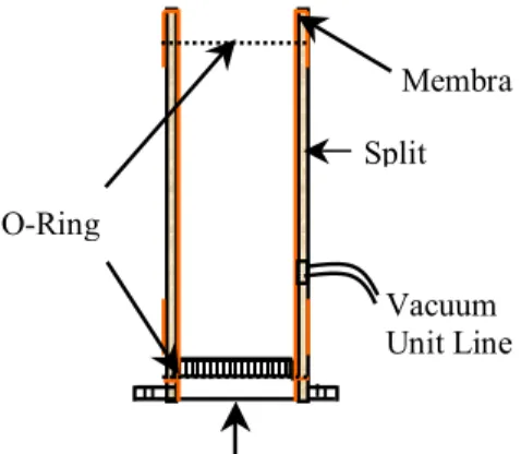
6.2.14 Stretch the membrane around the bottom plate. Place the split mold over the bottom plate and pull the membrane to the top of the mold as shown in step #1 in Figure 19.
Membrane
Split Mold
Bottom Plate
Figure 19. Granular sample preparation step #1
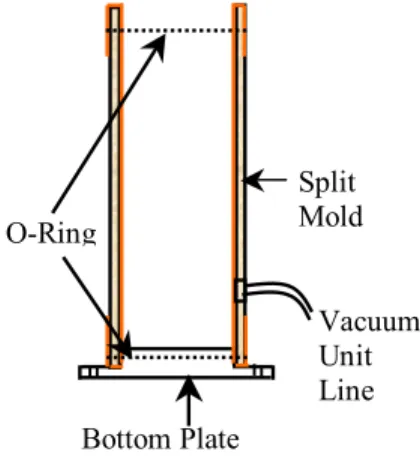
6.2.15 Stretch the membrane around the top outside edge of the mold and secure with an O-ring as shown in step #2 in Figure 20.
6.2.16 Flip the mold and stretch the membrane around the bottom outside edge of the mold and secure with an O-ring as illustrated in step #3 in Figure 21.
6.2.17 Connect the mold to a vacuum unit and apply suction such that the membrane will rest against the sides of the mold. Maintain the suction during the whole compaction process. This is illustrated in step #4 in Figure 22.
O-Ring
Bottom Plate
Figure 20. Granular sample preparation step
Split Mold
IRC
PROGRAM: EFFECTIVE DATE:
MARCH 03, 2006
FILE PATH:
Iso9000 on ‘Irc-public':\Urban Infrastructure
Rehabilitation\Work Instructions\Urban Roads
THIS DOCUMENT IS NOT CONTROLLED, UNLESS
THE ABOVE QA SIGNATURE IS IN RED INK.
Page 18 OF
46
Bottom Plate
O-Ring
Split
Mold
Membrane
Figure 21. Granular sample preparation step
Vacuum
Unit
Line
O-Ring
Bottom Plate
Split
Mold
Figure 22. Granular sample preparation step #4
6.2.18 Remove one of the porous stones from water (step 6.2.7) and insert it inside the compaction mold on top of the bottom plate as shown in step #5 in Figure 23.
6.2.19 Remove the wet soil from the Hobart mixer (step 6.2.12), thoroughly hand mix it and divide it into eight equal portions. The mass of each portion should be slightly greater than the amount recorded as “weight of soil mix/layer” shown in Data Block #2 in Figure A5. Place each portion in a container and seal it to minimize moisture loss.
6.2.20 Using one of the wet mix portions produced by step 6.2.19, scoop a mass of soil equal to the “weight of soil mix/layer” identified in Data Block #2 and pour it inside the mold as shown in step #6 in Figure 24. Shake the material with a spatula and tap it with a flattened end rod to evenly distribute the soil mass across the porous stone surface.
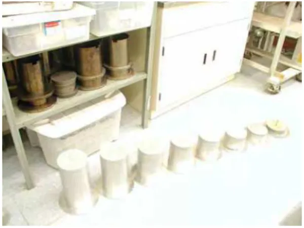
6.2.21 Eight aluminum cylindrical adapters (details shown in Figures 7 and 25), each of a progressively shorter length to provide a compacted layer thickness of 38 mm (1.5 in.), are used to ensure that the compaction process
DOCUMENT TITLE: REVISION #2
Institute for Research in
Construction
Resilient Modulus and Permanent Deformation Test
for Unbound Materials
DRAFT # 1
PROGRAM:
IRC
EFFECTIVE DATE: MARCH 03, 2006
produces layers with equal thickness and uniform density across the overall length of the test specimen. Insert the tallest adapter inside the mold on top of the first soil layer and compact it using the mechanical vibrator as depicted in step #7 in Figure 26.
6.2.22 Repeat the process described in step 6.2.21 with each subsequent adapter (going from the second tallest to the shortest) until all eight layers have been compacted.
O-Ring
Membra
Split
Bottom Plate and Porous
Bottom
Porous
Vacuum
Unit Line
O-Ring
Bottom
Split
Material
Figure 23. Granular sample preparation step #5
Vacuum
Unit Line
Figure 24. Granular sample preparation step #6
6.2.23 During the compaction of the last layer (#8), place the metal spacer shown in Figure 10 between the soil layer and the last adapter. This step will ensure that the top surface of the compacted specimen produced is smooth and flat (i.e. not inclined).
6.2.24 During steps 6.2.22 and 6.2.23, it is important to stop compacting once the flange of the cylindrical adapter reaches the edge of the compaction mold, otherwise any further vibration will cause water loss even if the layer is no longer compacting.
FILE PATH:
Iso9000 on ‘Irc-public':\Urban Infrastructure
Rehabilitation\Work Instructions\Urban Roads
THIS DOCUMENT IS NOT CONTROLLED, UNLESS
THE ABOVE QA SIGNATURE IS IN RED INK.
Page 19 OF
PROGRAM:
IRC
EFFECTIVE DATE: MARCH 03, 2006
6.2.25 Use the remaining wet soil for initial moisture content determination. The amount of material used in this step should not be less than 500 g to obtain a correct estimate of the water content. The information should be entered in the appropriate cells identified under the “Before Mr test” fields in Data Block #4 of Figure A5.
Figure 25. Eight adaptors used for compaction
Vibrator
Material for First Layer
Bottom Plate and Porous Stone
Tallest Adapter
Split Mold
Figure 26. Granular sample preparation step #7
6.2.26 Upon completing compaction of the test specimen, place the second porous stone on top of the last compacted layer. Pull the rubber membrane from the sides of the compaction mold as shown in Figure 27.
FILE PATH:
Iso9000 on ‘Irc-public':\Urban Infrastructure
Rehabilitation\Work Instructions\Urban Roads
THIS DOCUMENT IS NOT CONTROLLED, UNLESS
THE ABOVE QA SIGNATURE IS IN RED INK.
Page 20 OF
DOCUMENT TITLE: REVISION #2
Institute for Research in
Construction
Resilient Modulus and Permanent Deformation Test
for Unbound Materials
DRAFT # 1
PROGRAM:
IRC
EFFECTIVE DATE: MARCH 03, 2006
Figure 27. Granular sample preparation step #8
6.2.27 Unfasten the screws joining the two haves of the split mold and remove it as illustrated in Figure 28. 6.2.28 Use the rubber membrane and O-rings at the top and bottom of the test specimen to seal it.
6.2.29 Mount the compacted specimen onto the sample carrying assembly as shown in Figure 29.
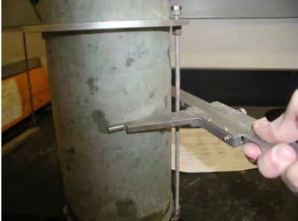
6.2.30 Record the weight of the sample and measure its diameter and height as shown in Figures 30 and 31. Enter these measurements in their respective cells within Data Blocks #4 and #5.
Figure 28. Granular sample preparation step #9
FILE PATH:
Iso9000 on ‘Irc-public':\Urban Infrastructure
Rehabilitation\Work Instructions\Urban Roads
THIS DOCUMENT IS NOT CONTROLLED, UNLESS
THE ABOVE QA SIGNATURE IS IN RED INK.
Page 21 OF
PROGRAM:
IRC
EFFECTIVE DATE: MARCH 03, 2006
Figure 29. Granular sample preparation step #10
Figure 30. Granular sample preparation step #11
Figure 31.
Granular sample preparation step #12
6.2.31 Transport the sample to the location where the Mr – PD Test will be conducted. Set up the specimen inside the
triaxial chamber as per the steps described in section 7 below.
FILE PATH:
Iso9000 on ‘Irc-public':\Urban Infrastructure
Rehabilitation\Work Instructions\Urban Roads
THIS DOCUMENT IS NOT CONTROLLED, UNLESS
THE ABOVE QA SIGNATURE IS IN RED INK.
Page 22 OF
DOCUMENT TITLE: REVISION #2
Institute for Research in
Construction
Resilient Modulus and Permanent Deformation Test
for Unbound Materials
DRAFT # 1
PROGRAM:
IRC
EFFECTIVE DATE: MARCH 03, 2006
7. Sample setup and testing
7.1 The sample setup and testing procedure described herein is the same for both granular and cohesive specimens. 7.2 Place the triaxial chamber base plate inside the bay of the loading frame.
7.3 Place the carrying assembly holding the compacted specimen on the base plate of the triaxial chamber and center it over the plate. Detach the compacted specimen from the carrying assembly and remove the assembly away from the loading frame.
7.4 Slip the bottom O-ring mounted on the specimen onto the pedestal of the chamber base plate to secure the test specimen to the base plate.
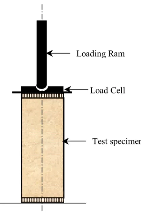
7.5 Centre the load cell on top of the compacted specimen. Lower the ram of the loading frame until it touches the top of the load cell as shown in Figure 32. Do not connect the load cell to the data acquisition system at this stage yet. This step is only intended to ensure that the loading ram of the frame is adequately aligned with the axis of the test specimen.
7.6 After the alignment check described in step 7.5 is performed, remove the load cell from the top of the specimen and lift up the loading ram an adequate distance to enable the positioning of the plate carrying the sensors’ holders around the test specimen.
7.7 Re-position the load cell on top of the specimen again and adjust the two metal flaps connected to it to press against the LVDTs’ rods as shown in Figure 33.
Loading Ram
Load Cell
Test specimen
Figure 32. Sample setup step #7.5
7.8 Using a small screwdriver, manually adjust the LVDT core to enable measurement of the vertical deformation to the maximum possible within the linear range of the device. This step, which is illustrated in Figure 33, should be performed for both LVDTs that are mounted 180 degrees diametrically opposite about the specimen’s axis.
FILE PATH:
Iso9000 on ‘Irc-public':\Urban Infrastructure
Rehabilitation\Work Instructions\Urban Roads
THIS DOCUMENT IS NOT CONTROLLED, UNLESS
THE ABOVE QA SIGNATURE IS IN RED INK.
Page 23 OF
PROGRAM:
IRC
EFFECTIVE DATE: MARCH 03, 2006
Figure 33. Sample preparation step #7.8
7.9 Connect the lead wires of the internal load cell and the LVDTs to the data acquisition system.
7.10 Plug in the external pressure transducer to the chamber base plate and connect its lead wire to the data acquisition system.
7.11 Raise the loading ram a further distance and place the chamber plexi-glass shell around the test specimen. Wipe the top of the plexi-glass cylinder with a clean cloth and place the cover plate of the triaxial chamber without disturbing the sample.
7.12 Lower the loading ram until it touches the top of the internal cell. Ensure that the loading ram is centrally positioned on the top of the test specimen. The success of this step is contingent upon achieving a good alignment as previously described in step 7.5.
7.13 Connect the pressure line that supplies air to the triaxial chamber and apply the confining pressure desired to reflect in-situ stress conditions.
7.14 Use the auto-zero offset feature in the data acquisition system to zero the ram and load cell readings. This will provide a base line (reference) for subsequent measurements. Lower the loading frame and bring the ram into contact with the internal load cell. Apply a constant load of magnitude equal to 10% of the desired repetitive load. Maintain this static load throughout the test duration.
7.15 Select the desired repetitive load level (from a number of alternatives made available by the test software) and commence the test.
7.16 Save the test results obtained in the PC hard drive (or a CD). The name of the electronic file containing these results is the one that should be entered in the sample preparation sheet shown in Figures A4 and A5 of Appendix A (i.e. the “MTS specimen #” field within Data Block #1).
7.17 After the test is completed, disassemble the triaxial chamber and weigh the test specimen. Record this weight as the “Total weight of sample immediately after test” shown in Data Block #5.
7.18 Measure the specimen diameter and height and record these measurements in Data Block #4.
7.19 Determine the final water content of the sample as per ASSHTO T265. Record this information under the “After Mr test” fields within Data Block #4.
7.20 Upon entering all the information displayed in Data Blocks #4 and #5, the spreadsheet (Figure A4 or A5) automatically computes all the values shown in Data Block #7. The “γd” and “m.c.%” refer to the actual dry
density and moisture content conditions achieved. The “D” and “H” represent the average sample diameter and height, respectively. These entries are later used for analysis of test results.
FILE PATH:
Iso9000 on ‘Irc-public':\Urban Infrastructure
Rehabilitation\Work Instructions\Urban Roads
THIS DOCUMENT IS NOT CONTROLLED, UNLESS
THE ABOVE QA SIGNATURE IS IN RED INK.
Page 24 OF
DOCUMENT TITLE: REVISION #2
Institute for Research in
Construction
Resilient Modulus and Permanent Deformation Test
for Unbound Materials
DRAFT # 1 PROGRAM:
IRC
EFFECTIVE DATE: MARCH 03, 2006Part II
Data Reduction and Analysis of Test Results
FILE PATH:
Iso9000 on ‘Irc-public':\Urban Infrastructure
Rehabilitation\Work Instructions\Urban Roads
THIS DOCUMENT IS NOT CONTROLLED, UNLESS
THE ABOVE QA SIGNATURE IS IN RED INK.
Page 25 OF
PROGRAM:
IRC
EFFECTIVE DATE: MARCH 03, 2006
1. Calculation of mechanical properties
1.1 The Mr – PD test described in Part I is carried out for a period of one hour. This produces 3600 repetitive axial
load cycles each having a load duration of 0.1 seconds and a rest period of 0.9 seconds as illustrated in Figure 34a. Each load cycle has three segments
The first segment, which lasts for 0.05 seconds, represents the loading portion of the cycle. The second segment, which lasts for 0.05 seconds, represents the unloading curve of the cycle. The third segment represents the rest period.
1.2 The axial deformation signal recorded by the LVDT(s), corresponding to the repetitive applied load, is depicted in Figure 34b. The deformation response in Figure 34b is divided into two parts
An elastic (resilient or recoverable) deformation component A permanent (plastic) deformation component.
1.3 Using the definitions given in steps 1.1 and 1.2, the following parameters are to be computed for every load/deformation cycle.
Divide the amplitude of the axial load signal by the specimen x-sectional area to obtain the maximum deviator stress, σdmax.
Divide the constant static load, shown as 10% of maximum load in Figure 34a, of the axial load signal by the specimen x-sectional area to obtain the minimum deviator stress, σdmin.
Calculate the cyclic deviator stress as: σdmax - σdmin = σdc
Divide the elastic deformation component by the specimen height to obtain the percentage elastic strain, εr.
Divide the plastic deformation component by the specimen height to obtain the percentage plastic strain, εp.
Calculate the percentage total strain as: εT = εr + εp.
Calculate the resilient modulus parameter as Mr = σdmax / εr.
1.4 The process of computing the parameters listed in step 1.3 above can be automated by using any spreadsheet software, such as Microsoft Excel®. An example displaying these calculations using the output from the Mr – PD
test is shown in Figure 35. Definitions of the various columns shown in this figure are as follows: Column A is the number of load cycle for which the mechanistic properties are computed. Column B is the percentage elastic strain obtained for each load cycle.
Column C is the computed resilient modulus for each load cycle.
Column D is the accumulated total strain (%) generated by summing the contribution of each cycle, e.g., the number in cell D3 (0.09461217) refers to the % total strain accumulated in cycle 1 whereas the number in D4 (0.123450529) refers to the sum of the % total strain accumulated in cycles 1 and 2.
Column E is the computed maximum deviator stress for each load cycle.
Column F is the accumulated permanent strain (%) generated by summing the contribution of each cycle, e.g., the number in cell F3 (0.068533725) refers to the % permanent strain accumulated in cycle 1 whereas the number in F4 (0.09243954) refers to the sum of the % permanent strain accumulated in cycles 1 and 2. Column G is the computed minimum deviator stress for each load cycle.
Column H is the calculated cyclic deviator stress for each load cycle. Column I is a repeat of column D.
Column J is a repeat of column F. Column K is a repeat of column B.
1.5 Other parameters that need to be identified for later use in the RUC design software include the following: MrMAX, which corresponds to the maximum Mr value obtained during the test.
MrMIN, which corresponds to the minimum Mr value obtained during the test.
FILE PATH:
Iso9000 on ‘Irc-public':\Urban Infrastructure
Rehabilitation\Work Instructions\Urban Roads
THIS DOCUMENT IS NOT CONTROLLED, UNLESS
THE ABOVE QA SIGNATURE IS IN RED INK.
Page 26 OF
DOCUMENT TITLE: REVISION #2
Institute for Research in
Construction
Resilient Modulus and Permanent Deformation Test
for Unbound Materials
DRAFT # 1
PROGRAM:
IRC
EFFECTIVE DATE: MARCH 03, 2006
Mro, which represents the Mr of the first load cycle.
Mre, which represents the average Mr of all load cycles. This value is the computed average of all Mr values
exclusive of the first 10 load cycles.
IStrain, which corresponds to the percentage total strain of the first load cycle (i.e. the point at which strain hardening starts, see Figure 35).
IStress, which corresponds to the maximum deviator stress of the first load cycle (i.e. the point at which strain hardening starts, see Figure 35).
FStrain, which corresponds to the percentage total strain of the 100-load cycle (i.e. the point at which strain hardening ends, see Figure 35).
FStress, which corresponds to the maximum deviator stress of the 100-load cycle (i.e. the point at which strain hardening ends, see Figure 35).
1.6 Using the three sets of data obtained from step 1.4 (referred to as First Data Set, Second Data Set and Third Data Set in Figure 35) and any commercially available statistical software, such as TableCurve®, perform regression analysis to generate the three mechanistic equations that describe the material response as follows:
With column B as the independent variable (X) and column C as the dependent variable (Y), obtain the M – Equation (resilient modulus equation).
With column D as the independent variable and (X) column E as the dependent variable (Y), obtain the K – Equation (hardening equation). Values inclusive of load cycles 0 to 100 only should be used for obtaining this equation.
With column J as the independent variable (X) and column I as the dependent variable (Y), obtain the
E
– Equation (strain equation).1.7 In performing the regression analysis described in step 1.6 above, only the equation forms provided in Table A2 should be used for postulating the three relationships (i.e. M–, K–,
E
– equations). These equation forms are the only ones that are currently implemented in the RUC design software. Moreover, the equation number (shown in the second column of Table A2) is also an input that the RUC design software requires for performing analysis exercises.2. NRC macro
2.1 The computations described in steps 1.3 and 1.4 are incorporated in an electronic Microsoft Excel® macro to help users of the RUC Restoration Guide obtain the mechanical properties from the results of the Mr – PD test. This
macro automatically performs all the calculations described in steps 1.3 and 1.4 above. However, step 1.6 requires the utilization of a statistical software to postulate the three characteristic equations. An electronic copy of the NRC macro developed in this project is provided with the Guide.
2.2 During the Mr – PD test, a selected number of the loading cycles (and the corresponding deformation cycles) are
acquired and saved in the electronic file containing the results of the test. This set of data was found to be quite adequate for describing the stress–strain response of the tested specimen. Moreover, the limited number of cycles retrieved enables efficient handling of the test results for further data reduction and analysis.
2.3 The MTS data acquisition software, used at NRC, was set to acquire the test data using the collection scheme shown in Table 2. Within each loading cycle, the software was set to collect a total of 166 measurement points. 2.4 Using the collection scheme of Table 2 and the terms defined in steps 1.1 and 1.2, the NRC macro can be utilized
to perform data reduction of the Mr – PD test results to obtain the parameters listed in steps 1.3 and 1.5. Figure A7
shows the main macro sheet where the macro can be invoked by pressing the button labeled “Compute Stresses and Mr”. The macro is based on the format of the raw data shown in Figure A6. Upon pressing the button labeled “Compute Stresses and Mr”, the macro prompts the user through a dialog window to open the raw data file as shown in Figure A8.
2.5 The macro also enables the user to plot the LVDT (deformation) data collected during the test. This feature, which is shown in Figure A9, gives the user the flexibility of choosing which portion of the data to be analyzed (only one LVDT data set or both sets), and also provides a means for eliminating erroneous data prior to starting the data reduction process. Using the “Userform1” window of Figure A9, the user enters the test specimen properties needed to perform computations of the stresses, strains and Mr parameters. The specimen dimensions required to
FILE PATH:
Iso9000 on ‘Irc-public':\Urban Infrastructure
Rehabilitation\Work Instructions\Urban Roads
THIS DOCUMENT IS NOT CONTROLLED, UNLESS
THE ABOVE QA SIGNATURE IS IN RED INK.
Page 27 OF
PROGRAM:
IRC
EFFECTIVE DATE: MARCH 03, 2006
be input in the “Userform1” window of Figure A9 can be picked up from Data Block #7 in the sample preparation sheet (Figures A4 and A5).
2.6 Another feature of the NRC macro is that it gives the user the option of plotting the PD curves into a separate file. This option enables the user to compare between the responses of different tested materials.
2.7 The steps involved in using the macro to perform the analysis described in the previous steps, can be summarized as follows:
2.7.1 Open the Excel file containing the macro sheet by clicking on the macro file name. The window shown in Figure A7 will appear. Definitions of the various data columns shown in this sheet are given in Table A1. These data columns correspond to the raw data columns contained in the electronic file obtained from the test (see Figure A6).
2.7.2 Open the specimen’s raw data file obtained from the test by pressing the button labeled “Compute Stresses and Mr” in Figure A7. The open file dialog box appears as shown in Figure A8. Locate the raw data file and open
it. The dialog window “Userform1” of Figure A9 appears.
2.7.3 Select the LVDT data desired to be plotted (the user can choose from among three options: Both LVDTs; LVDT1; LVDT2) and press the button labeled “Draw Chart”. This step will create a plot of the deformation measured using the specified LVDT set. Examination of the plotted deformation data using the three available options and the notes taken during the test will assist the user on deciding which LVDT data set to keep for subsequent analysis.
2.7.4 After deciding on which LVDT data set to keep for further analysis, enter test specimen dimensions in the sample properties’ fields (height and diameter). These properties are obtained from Data Block #7 in the sample preparation sheet (Figure A 4 or Figure A5). Keep the “Number of average points” as 50 and click on the button labeled “Next” in Figure A9. The macro will run for few seconds and the dialog window “Add curves” shown in Figure A10 will appear.
2.7.5 The window appeared in step 2.7.4 will give the user the option of saving a copy of the PD curve (and the Mr
curve) of the analyzed test specimen in a new Excel file or add it to an existing file. The user also has the option of exiting from this window without saving a copy of the PD/Mr curves (by pressing the “Exit” button).
Examples showing the PD and Mr curves are displayed in Figures A12 and A13, respectively.
2.7.6 Upon execution of step 2.7.5, the macro will run for few seconds and two Excel Work books will be created. The first “Work Book”, labeled Book 1, contains a number of excel sheets and charts that display different information pertaining to the mechanistic properties of the analyzed test specimen. Sheet 2 of this Work Book is the equivalent of Figure 35 described earlier in step 1.4. The chart labeled “stress-strain char. curve” represents the stress – strain characteristic relationship of the tested material (see example shown in Figure A11).
2.7.7 The second Work Book, Book 2, contains copies of the PD and Mr plots of the analyzed specimen.
2.7.8 Information contained in Sheet 2 of Book 1 represents the input required by the RUC design software to perform design and analysis exercises. This information also represents the source from which the three characteristic equations (evolution of the resilient modulus with load applications, the M–Equation; the hardening behaviour of the materials, the K–Equation; and the decomposition of the total strain into its elastic and plastic components, the
E
–Equation) of the material were derived.FILE PATH:
Iso9000 on ‘Irc-public':\Urban Infrastructure
Rehabilitation\Work Instructions\Urban Roads
THIS DOCUMENT IS NOT CONTROLLED, UNLESS
THE ABOVE QA SIGNATURE IS IN RED INK.
Page 28 OF
DOCUMENT TITLE:
Institute for Research in
Construction
Resilient Modulus and Permanent Deformation Test
REVISION #2 DRAFT # 1
for Unbound Materials
GRAM:
IRC
EFFECTIVE MARCH 03, 2 PRO DATE: 006Axial
Load
Signal
(lb)
10% Maximum Load
Segment
0.05
Segment
#2
#1
0.1
0.9
Time
Segment #3
(a)
Axial
Defo
rmation
Signal
(mm)
Elastic Deformation
Permanent (Plastic)
Deformation
Time
0
.1
0.05
1.0
1.05
1
.1
(b)
Figure 34. Typical load and deformation pulses during M
r– PD test (1 in. = 25.4 mm)
FILE PATH:
Iso9000 on ‘Irc-public':\Urban Infrastructure
Rehabilitation\Work Instructions\Urban Roads
THIS DOCUMENT IS NOT CONTROLLED, UNLESS
THE ABOVE QA SIGNATURE IS IN RED INK.
Page 29 OF
PROGRAM:
IRC
EFFECTIVE DATE: MARCH 03, 2006
Mr
oFigure 35. Calculation spreadsheet to obtain mechanical properties
IStrain
IStress
FStrain
X
Third
Data
Set
Y
FStress
X
Second
Data
Set
Y
X
Y
First
Data
Set
FILE PATH:Iso9000 on ‘Irc-public':\Urban Infrastructure
Rehabilitation\Work Instructions\Urban Roads
THIS DOCUMENT IS NOT CONTROLLED, UNLESS
THE ABOVE QA SIGNATURE IS IN RED INK.
Page 30 OF
DOCUMENT TITLE: REVISION #2
Institute for Research in
Construction
Resilient Modulus and Permanent Deformation Test
for Unbound Materials
DRAFT # 1
PROGRAM:
IRC
EFFECTIVE DATE: MARCH 03, 2006
Table 2. Data acquisition collection scheme
Load Cycles
Segments*
From To From To
0 10 0 29
30 38 88 111
80 88 238 261
100 108 298 321
200 208 598 621
300 308 898 921
400 408 1198 1221
500 508 1498 1521
600 608 1798 1821
700 708 2098 2121
800 808 2398 2421
900 908 2698 2721
1000 1008 2998 3021
1100 1108 3298 3321
1200 1208 3598 3621
1300 1308 3898 3921
1400 1408 4198 4221
1500 1508 4498 4521
2000 2008 5998 6021
2500 2508 7498 7521
3000 3008 8998 9021
3500
3508
10 498
10 521
*Segments refer to the three segments comprising each individual load cycle (See definitions in step 1.1)
FILE PATH:
Iso9000 on ‘Irc-public':\Urban Infrastructure
Rehabilitation\Work Instructions\Urban Roads
THIS DOCUMENT IS NOT CONTROLLED, UNLESS
THE ABOVE QA SIGNATURE IS IN RED INK.
Page 31 OF
PROGRAM:
IRC
EFFECTIVE DATE: MARCH 03, 2006
Bottom porous stone
Pressure line
Chamber base plate
Test specimen
LVDT assembly
Chamber top plate
Membrane
External wall of tri-axial chamber
Top porous stone
Hydraulic actuator
Sensors lead wires
Tie rod
Figure A1. Details of triaxial test chamber for cohesive material
FILE PATH:
Iso9000 on ‘Irc-public':\Urban Infrastructure
Rehabilitation\Work Instructions\Urban Roads
THIS DOCUMENT IS NOT CONTROLLED, UNLESS
THE ABOVE QA SIGNATURE IS IN RED INK.
Page 32 OF
Institute for Research in
Construction
DOCUMENT TITLE:
Resilient Modulus and Permanent Deformation Test
for Unbound Materials
REVISION #2 DRAFT # 1
PROGRAM: EFFECTIVE DATE:
IRC
MARCH 03, 2006Hydraulic actuator
Chamber top plate
Top porous stone
LVDT assembly
Tie rod
External wall of tri-axial chamber
Test specimen
Membrane
Bottom Plate
Bottom porous stone
Sensors lead wires
Chamber base plate
Pressure line
Figure A2. Details of triaxial test chamber for granular material
FILE PATH:
Iso9000 on ‘Irc-public':\Urban Infrastructure
Rehabilitation\Work Instructions\Urban Roads
THIS DOCUMENT IS NOT CONTROLLED, UNLESS
THE ABOVE QA SIGNATURE IS IN RED INK.
Page 33 OF
PROGRAM:
IRC
EFFECTIVE DATE: MARCH 03, 20066.52”
2.906
8.898
Extrusion Ram2.906
3.49”
Extrusion Mold9”
Specimen Mold2.906
3.49”
Loading Ram3”
3.54”
4.53”
0.79”
Figure A3. Apparatus for preparation of cohesive samples (1 in. = 25.4 mm)
FILE PATH:
Iso9000 on ‘Irc-public':\Urban Infrastructure
Rehabilitation\Work Instructions\Urban Roads
THIS DOCUMENT IS NOT CONTROLLED, UNLESS
THE ABOVE QA SIGNATURE IS IN RED INK.
Page 34 OF
Figure A4. Sample preparation sheet for cohesive materials
FILE PATH:
Iso9000 on ‘Irc-public':\Urban Infrastructure
Rehabilitation\Work Instructions\Urban Roads
THIS DOCUMENT IS NOT CONTROLLED, UNLESS
THE ABOVE QA SIGNATURE IS IN RED INK.
Page 35 OF
Figure A5. Sample preparation sheet for granular materials
FILE PATH:
Iso9000 on ‘Irc-public':\Urban Infrastructure
Rehabilitation\Work Instructions\Urban Roads
THIS DOCUMENT IS NOT CONTROLLED, UNLESS
THE ABOVE QA SIGNATURE IS IN RED INK.
Page 36 OF
FILE PATH:
Iso9000 on ‘Irc-public':\Urban Infrastructure
Rehabilitation\Work Instructions\Urban Roads
THIS DOCUMENT IS NOT CONTROLLED, UNLESS
THE ABOVE QA SIGNATURE IS IN RED INK.
Page 37 OF
46
Figure A6. Typical raw data file obtained from M
r– PD test
Figure A7. Main macro sheet
FILE PATH:
Iso9000 on ‘Irc-public':\Urban Infrastructure
Rehabilitation\Work Instructions\Urban Roads
THIS DOCUMENT IS NOT CONTROLLED, UNLESS
THE ABOVE QA SIGNATURE IS IN RED INK.
Page 38 OF
FILE PATH:
Iso9000 on ‘Irc-public':\Urban Infrastructure
Rehabilitation\Work Instructions\Urban Roads
THIS DOCUMENT IS NOT CONTROLLED, UNLESS
THE ABOVE QA SIGNATURE IS IN RED INK.
Page 39 OF
46
Figure A8. Open file menu window
Figure A9. Dialog window for plotting LVDT measurements
FILE PATH:
Iso9000 on ‘Irc-public':\Urban Infrastructure
Rehabilitation\Work Instructions\Urban Roads
THIS DOCUMENT IS NOT CONTROLLED, UNLESS
THE ABOVE QA SIGNATURE IS IN RED INK.
Page 40 OF
Figure A10. Saving PD and M
rplots to an existing file (1 in. = 25.4 mm)
FILE PATH:
Iso9000 on ‘Irc-public':\Urban Infrastructure
Rehabilitation\Work Instructions\Urban Roads
THIS DOCUMENT IS NOT CONTROLLED, UNLESS
THE ABOVE QA SIGNATURE IS IN RED INK.
Page 41 OF
FILE PATH:
Iso9000 on ‘Irc-public':\Urban Infrastructure
Rehabilitation\Work Instructions\Urban Roads
THIS DOCUMENT IS NOT CONTROLLED, UNLESS
THE ABOVE QA SIGNATURE IS IN RED INK.
Page 42 OF
46
Figure A11. Typical stress – strain relationship for tested granular material (1 psi =6.894 kPa)
Figure A12. Typical PD plot for granular specimen
FILE PATH:
Iso9000 on ‘Irc-public':\Urban Infrastructure
Rehabilitation\Work Instructions\Urban Roads
THIS DOCUMENT IS NOT CONTROLLED, UNLESS
THE ABOVE QA SIGNATURE IS IN RED INK.
Page 43 OF
Figure A13: Resilient modulus plot for granular specimen
FILE PATH:
Iso9000 on ‘Irc-public':\Urban Infrastructure
Rehabilitation\Work Instructions\Urban Roads
THIS DOCUMENT IS NOT CONTROLLED, UNLESS
THE ABOVE QA SIGNATURE IS IN RED INK.
Page 44 OF
Table A1. Description of specimen’s raw data* (1 in = 25.4 mm)
Column Title Definition Units
A Time Time interval at which test data is collected. Seconds
B Empty Column
C Axial Segment Count The number identifying the segment within the loading cycle e.g. 0, 1 and 2 segments’ data refer to the data points collected during the first repetitive load cycle.
#
D Axial Ram LVDT Deformation measurement recorded by the MTS LVDT (an external sensor mounted inside the MTS loading frame).
mm
E Axial Ram Force Load measurement recorded by the MTS load cell (an external load cell mounted inside the MTS loading frame).
lbf
F Axial Load Cell_2 Load measurement recorded by the internal
load
cell that is mounted on the top of the test
specimen.
lbf
G Axial LVDT-1 Deformation measurement recorded by LVDT-1 sensor connected to the test specimen.
mm
H Axial LVDT-2 Deformation measurement recorded by LVDT-2 sensor connected to the test specimen.
mm
I
Empty Column
J
Empty Column
K Axial Pressure
Confining pressure measurements.
lbf / in2*The format of the data shown in Figure A7 is essential for the macro to run i.e. location of the various columns and rows shown should be kept as illustrated.
FILE PATH:
Iso9000 on ‘Irc-public':\Urban Infrastructure
Rehabilitation\Work Instructions\Urban Roads
THIS DOCUMENT IS NOT CONTROLLED, UNLESS
THE ABOVE QA SIGNATURE IS IN RED INK.